Redispatching active and reactive powers using a
limited number of control actions
Florin Capitanescu and Louis Wehenkel, Member, IEEE
Abstract—This paper deals with some essential open questions in the field of optimal power flow (OPF) computations, namely: the limitation of the number of controls allowed to move, the trade-off between the objective function and the number of controls allowed to move, the computation of the minimum number of control actions needed to satisfy constraints, and the determination of the sequence of control actions to be taken by the system operator in order to achieve its operation goal. To address these questions, we propose approaches which rely on the computation of sensitivities of the objective function and inequality constraints with respect to control actions. We thus determine a subset of controls allowed to move in the OPF, by solving a sensitivity-based mixed integer linear programming (MILP) problem. We study the performances of these approaches on three test systems (of 60, 118, and 618 buses) and by considering three different OPF problems important for a system operator in emergency and/or in normal states, namely the removal of thermal congestions, the removal of bus voltage limits violation, and the reduction of the active power losses.
Index Terms—mixed integer linear programming, nonlinear programming, optimal power flow
I. INTRODUCTION A. Motivation
I
N order to provide system operators (SOs) with useful guidelines, OPF computations should address properly a certain number of questions. Among the still open questions, we focus on the following ones in this paper [1]–[5]:1) SOs seek for a small number of control actions to implement over a limited time period in both emergency state (e.g. to manage congestions and salvage the system integrity) and normal state (e.g. to improve a predefined operation goal).
2) A more general and useful information for the SOs is the trade-off between the objective function and the number of control actions used in the optimization.
3) In the emergency state, an essential information for a SO is the minimum number of control actions that is required in order to remove constraints’ violations. This information allows the SO to assess whether enough time is available to refine the control actions to salvage the system at a lower cost.
The authors acknowledge the financial support of the FP7 project PEGASE funded by the European Commission.
This paper presents research results of the Belgian Network DYSCO, funded by the Interuniversity Attraction Poles Programme, initiated by the Belgian State, Science Policy Office. The scientific responsibility rests with the authors.
F. Capitanescu and L. Wehenkel are with the Department of Electrical Engineering and Computer Science, University of Li`ege, B4000 Li`ege, Belgium (e-mail: [email protected]; [email protected]).
4) The SOs need to appraise a sequence of control actions to take in order to reach their objectives, so as to assess the induced path on the objective and the constraints (e.g. to avoid exacerbating the already violated con-straints and to avoid inducing other severe constraint violations during operation).
This paper proposes approaches to address these four ques-tions by imposing bounds on the number of control acques-tions within the OPF formulation.
B. Related work
There is no straightforward way to formulate the trade-off between the objective function and the number of con-trol actions used in the optimization in a conventional OPF computation. Indeed, most OPFs use the whole set of control means to solve the problem and very often (almost) all of them will have moved at the optimum. The difficulty of limiting the number of controls moved in an OPF calculation is due to the fact that (i) most control variables participate both to improving the objective and to satisfying the constraints, and (ii) the control actions are not easy to rank in terms of usefulness because the effectiveness of an action is not necessarily related to its amount of variation [1].
The most widely used approach to limit the number of control actions in the OPF (we call this the OPF-LNC problem in the sequel), consists in specifying by hand the controls allowed to participate in the OPF [1]–[3], typically based on human judgment and a first run of the OPF where all possible controls are allowed to move. A few heuristic approaches proposed so far to automate this more or less, rely on either (i) using sensitivities of the objective and constraints to control movements [6] to pre-select them, (ii) approximating the integer constraint on the maximal number of controls allowed to move [7], [8], (iii) using mathematical programming with equilibrium constraints [8], (iv) embedding the dc approxi-mation of the OPF into a MILP and focusing on topological actions [9], [10], and (v) combining first order sensitivities and MILP [11].
As regards the OPF problem of determining the minimum number of control actions (which we call OPF-MNC in the sequel), only a heuristic approach has been proposed [3]. The objective function of this technique uses a linear “V” shaped curve for each control, with the same slope for all controls and the zero value of cost at the target initial control value.
Little research effort has been devoted so far to the de-termination of an optimal sequence of control actions [12], [13]. In [12] a recursive algorithm is used to compute the
sequence of reactive power controls to ensure voltage security. In [13] a model predictive control approach, using a dc power flow model, is used to compute the sequence of active power controls to alleviate thermal overloads in emergency state. C. Paper contribution and organization
In this paper we generalize the approach presented in [11] in three respects: (i) to address the OPF-LNC problem when the maximum number of control actions that the SO can take is insufficient to remove violated constraints, (ii) to address the closely related OPF-MNC problem of determining the minimum number of control actions to remove violated constraints, and (iii) to compute a sequence of control actions that the SO may take to safely reach its goal. We discuss algorithmic aspects of these approaches and we validate them extensively on OPF problems of broad interest, namely the removal of bus voltage limit violations, the removal of branch limit violations, and minimization of active power losses.
The rest of the paper is organized as follows. Section II recalls the formulation of the conventional OPF problem. Section III presents the assumptions and basic ideas of the proposed approaches. Section IV formulates the OPF-LNC problem in normal state. Section V formulates both OPF-LNC and OPF-MNC problems in emergency state. Section VI presents the proposed algorithms to the LNC and OPF-MNC problems. Section VII provides numerical results with the proposed approaches, and Section VIII concludes.
II. CONVENTIONALOPTIMALPOWERFLOW PROBLEM The conventional OPF problem can be written as follows:
min
x,uf (x, u) (1)
s.t. g(x, u) = 0 (2)
h(x, u) ≤ 0 (3)
u≤ u ≤ u, (4)
where x is the vector of state variables (i.e. the magnitude and the angle of voltage at all buses), u is the vector of control variables (e.g. generators active power, generators voltage (when controllable), Load Tap Changer (LTC) transformer ratios, shunt element reactances, load curtailment controls, phase shifters angle, etc.) and u (resp. u) is its corresponding vector of lower (resp. upper) bounds, f (·) is the objective function, g(·) and h(·) are vectors of functions which model equality and inequality constraints. Equality constraints (2) are essentially the ac bus power equations, inequality constraints (3) refer to operational limits (e.g. branch currents and voltage magnitudes) while inequality constraints (4) refer to physical limits of equipments (e.g. bounds on: generator active/reactive powers, LTCs transformer ratios, shunt reactances, phase shifter angles, etc.).
III. ASSUMPTIONS OF THE PROPOSED APPROACH A. Intuitive view of the problem
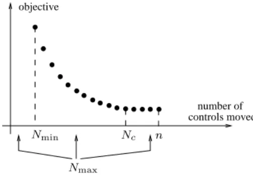
We first introduce the notations of five essential numbers of control actions that will be used in the paper:
controls movednumber of objective
Nmax
Nmin Nc n
Fig. 1. Objective function versus the number of controls allowed to move
• n is the total number of available controls defined in the conventional OPF (1)-(4);
• Nmin is the minimum number of controls required to move in order to yield a feasible solution;
• Nmaxis the maximum number of control actions that the SO can practically take in a given period of time in order to fulfill its objective;
• Nc is the minimal number of controls beyond which the objective can not be improved further, i.e. the number of controls which has effectively moved in the conventional OPF (1)-(4);
• N denotes generically any bound on the number of control actions for which the SO wishes to evaluate the optimal value of the objective function.
These notions are illustrated in Figure 1. Remark that the knowledge of the available time horizon for reaching the op-erating goal may be used by the SO to estimate the maximum number of control actionsNmax that it could implement, and hence to better assess the situation by analyzing the trade-off curve. Indeed, the part of the curve on the left ofNmaxshows the sub-optimality implied by using even smaller numbers of control moves and whether there is enough room of maneuver in the case where some control actions would fail, while the part on the right allows to assess the regret implied by the Nmax constraint. Ex-post consolidations of these information items may help the SO to justify investments in improved procedures and automatic devices liable to increaseNmax. B. Assumptions concerning the system behavior during the implementation of control actions
Our approaches provide the SO with the desired number of control actions to achieve its operation goal, the SO being responsible for the open-loop implementation of these actions. We make the following assumptions concerning the system behavior during the implementation of the control actions:
1) One control action is implemented at the time and during the implementation of the sequence of control actions the system state change is induced only by these control actions and the system automata reaction (e.g. frequency regulation, voltage regulation, etc.) to them1.
1This is a fair assumption given that the implementation of the control actions generally requires few minutes during which load and generation changes are normally negligible. However, the approaches could in principle be adapted so as to accommodate with any available load/generation forecasts over the concerned time-horizon.
2) After the application of each control action the system reaches a new equilibrium point and during the appli-cation of each control action the system does not lose stability2.
3) In real-time operation, the proposed approaches can rely on the updated outputs of the state estimator in order to take advantage of the changing operating conditions.
C. Operating objectives in emergency state and in normal state
System operators generally have different objectives in normal and in emergency3 states [2], [15]:
1) In normal state the objective is to improve a pre-defined performance measure related to security and/or economy (e.g. minimum power losses, maximize reactive power reserves, etc.) [2], [3]. We denote withfn this objective in normal state.
2) In emergency state the SOs’ aim is to remove as soon as possible the violated limits. Several objective functions can be thought of [2], [3]: minimum cost of corrective actions, minimum amount of controls deviations with respect to the base case, minimum number of control actions, minimum amount of limit violations, etc. How-ever, depending on the amount and type of violated limits, the time allowed for taking corrective actions, as well as the power system threat induced by these violations (e.g. cascading overloads, voltage instability, etc.), the SO may focus more on “keeping the lights on” than to minimize the cost of corrective actions. Thus, in Fig. 1 we distinguish among two different situations encountered in emergency state:
• IfNmax< Nminthen the violated limits can not be completely removed. We denote with fi
e the SO’s objective in this case. A reasonable objective is the minimization of the amount of limit violations. • If Nmax ≥ Nmin then the limit violations can be
removed. We denote with fv
e the SO’s objective in this case. It should be noted that in this case the trade-off curve contains two parts fi
e vs N ,
∀N ∈ {1, . . . , Nmin− 1} and fev vs N , ∀N ∈
{Nmin, . . . , Nmax}.
D. Outline of the proposed approach
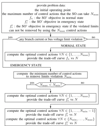
Figure 2 presents the outline of the proposed approach which summarizes the ideas discussed so far. In particular the difference between the output of the two operating modes (emergency and normal) is highlighted.
The following sections are devoted to the formulation of the sequence of optimization problems appearing in this flowchart and to the description of the proposed solution approaches.
2This can be checked by a time domain simulation program.
3In this work we consider that an emergency state is induced by some disturbance (e.g. line outage) which leads to branch overloads or bus voltage limit violations.
yes no
compute the minimum number of control actions yes
any branch current or bus voltage limit violation ? provide problem data:
NORMAL STATE no
EMERGENCY STATE
can not be removed by using the Nmaxcontrol actions
compute the optimal control actions∀N ∈ {1, . . . , Nmax}
provide the trade-off curve fnvs N
Nmax< Nmin?
compute the optimal control actions∀N ∈ {1, . . . , Nmin− 1}
compute the optimal control actions∀N ∈ {Nmin, . . . , Nmax}
compute the optimal control actions∀N ∈ {1, . . . , Nmax}
provide the trade-off curve fi
evs N
provide the trade-off curve fi
evs N
provide the trade-off curve fevvs N
to remove limits violation Nmin
the initial operating point
the maximum number of control actions that the SO can take Nmax
fn: the SO’ objective in normal state
fv
e : the SO’ objective in emergency state
fei: the SO’ objective in emergency state if the violated limits
Fig. 2. Outline of the proposed approach
IV. OPF-LNCPROBLEM FORMULATION IN NORMAL STATE A. OPF-LNC problem formulation
Since in the normal state all limits are satisfied the minimum number of control actions isNmin= 0 and hence there is no need to formulate the OPF-MNC problem.
The OPF-LNC problem can be compactly formulated as follows: fn= min x,u,sf (x, u) (5) s.t. g(x, u) = 0 (6) h(x, u) ≤ 0 (7) si(ui− u 0 i) ≤ ui− u0i ≤ si(ui− u0i), i = 1, . . . , n (8) n X i=1 si≤ N (9) si∈ {0, 1} i = 1, . . . , n, (10) where u = [u1, . . . , ui, . . . , un]T is the n-dimensional vec-tor of control variables, u = [u1, . . . , ui, . . . , un]T (resp.
u = [u1, . . . , ui, . . . , un]T) denotes its corresponding vector of lower (resp. upper) bounds, u0 = [u0
1, . . . , u0i, . . . , u0n]T is the vector of base case values of the control variables, s = [s1, . . . , si, . . . , sn]T is the vector of control variables statuses, andN is the specified maximum number of controls allowed to move.
Constraints (10) ensure that the status of any control is either 0 or 1. Constraints (8) impose bounds on control movements with respect to the base case. Observe that if the status of a control is equal to 1 (resp. 0) the latter is allowed to vary
between its bounds (resp. is frozen to its base case valueu0 i). Constraint (9) thus limits the number of controls that can be moved.
Note that controls can be classified according to the time required to change their output into very fast (or quasi-instantaneous) controls (e.g. load curtailment, shunt reactive power, transformer ratio, etc.) and comparatively slower con-trols (e.g. generator active power). Constraint (10) does not distinguish between fast and slow controls4. In order to treat
these classes of controls on the same basis the rate of change of slower controls in (8) may be reduced (e.g. by adapting the boundsui andui and/or defining several slices of control amount for slower controls, each slice having associated a status variable si).
Solving the OPF-LNC problem (5)-(10) for each possible value of N (i.e. ∀N ∈ {1, . . . , Nmax}) would allow to determine a trade-off curve of fn versus N , similar to the one illustrated on Fig. 1.
B. Computation of the sequence of control actions: problem formulation
The computation of the sequence of Nmax control actions can be formulated in a recursive manner and relies on the solution of the OPF-LNC problem obtained for increasing values ofN (N = 1, 2, . . . , Nmax): minf (xN, u1 C1, . . . , u N −1 CN−1, u N) (11) s.t. g(xN, u1 C1, . . . , u N −1 CN−1, u N) = 0 (12) h(xN, u1C1, . . . , u N −1 CN−1, u N ) ≤ 0 (13) sN i (ui− u0i) ≤ u N i − u0i ≤ s N i (ui− u0i), i = 1, . . . , n (14) uCk− u 0 Ck≤ u k Ck− u 0 Ck≤ uCk− u 0 Ck, k = 1, . . . , N − 1 (15) n X i=1 sN i ≤ N (16) sN i ∈ {0, 1}, i = 1, . . . , n (17) sN Ck = 1, k = 1, . . . , N − 1, (18)
where each set Ck (k = 1, . . . , N − 1) contains a single element, namely the index of the control that has additionally moved when solving the OPF-LNC problem forN = k.
Note that we allow for revising the changes imposed on the previousN −1 control actions, as modeled by constraints (15) and (18); the formulation may however be straightforwardly adapted so as to freeze the already committed controls at every step of the procedure.
This formulation can be interpreted as follows: given the previousN − 1 control actions (which are possibly allowed to change their magnitude at the next step) find theN th control action from the vector uN which leads to the best objective value and satisfies problem constraints.
4Alternatively the constraint (10) can be expressed in terms of the time needed for controls implementation (e.g. Pni=1siti ≤T where ti is the time needed to implement the control action i and T is the time period in which the SO wishes to fulfill its objective).
We denote with u1⋆
C1 − u0C1, . . . , uN ⋆CN − u 0
CN, ∀N ∈
{1, . . . , Nmax} the optimal sequence of control actions pro-vided by this optimization problem.
Let us notice that this formulation can be extended straight-forwardly to the OPF-MNC problem and the other variants of the OPF-LNC problem.
V. OPF-LNCANDOPF-MNCPROBLEMS FORMULATION IN EMERGENCY STATE
A. OPF-MNC problem formulation
The OPF-MNC problem which determines the minimum number of controls allowed to moveNminin order to remove violated limits can be compactly formulated as follows:
Nmin= minx ,u,s n X i=1 si (19) s.t. g(x, u) = 0 (20) h(x, u) ≤ 0 (21) si(ui− u0i) ≤ ui− u0i ≤ si(ui− u0i), i = 1, . . . , n (22) si ∈ {0, 1} i = 1, . . . , n, (23) B. OPF-LNC problem formulation withNmax< Nmin
In this case the OPF-LNC problem can be compactly formulated as follows: fi e= minx ,u,s,r1 Tr (24) s.t. g(x, u) = 0 (25) h(x, u) ≤ r (26) si(ui− u0i) ≤ ui− u0i ≤ si(ui− u0i), i = 1, . . . , n (27) n X i=1 si ≤ N (28) si∈ {0, 1} i = 1, . . . , n (29) r≥ 0, (30)
where positive relaxation variables (30) have been introduced in order to relax the inequality constraints (7). The objective (24) is the minimization of the amount of constraints violation in the sense of theL1 norm.
The trade-off curve fi
e versus N can be obtained af-ter solving the OPF-LNC problem (24)-(30) for ∀N ∈ {1, . . . , Nmax}. Clearly, since Nmax< Nmin the SO will not be able to completely clear the violated constraints.
C. OPF-LNC problem formulation withNmax≥ Nmin In this case the OPF-LNC problem has the same formulation as in normal state (see section IV).
The beforehand determination of Nmin provides useful information for the OPF-LNC problem (5)-(10) by helping to choose values ofN such that to avoid dealing with infeasible OPF-LNC problems, situations which arise forN < Nmin.
Solving the OPF-LNC problem (5)-(10) for each value of N in the range ∀N ∈ {Nmin, . . . , Nmax} allows to obtain the trade-off curvefv
VI. PROPOSED APPROACH TO THEOPF-LNCAND THE OPF-MNCPROBLEMS
A. Overview of the proposed approach
The OPF-MNC problem (19)-(23) and the OPF-LNC prob-lems (5)-(10) and (24)-(30) constitute mixed integer nonlin-ear programming problems (MINLPs). However, it is widely agreed that state of the art MINLP solvers (e.g. branch and bound, Benders decomposition, etc.) are not yet able to cope with very large size problems with a large number of integer variables, such as OPF applications for real-life power systems, especially under the stringent computing time requirements of real-time operation. To fix ideas, note that even for the moderate size problem withn = 39 and N = 10 that we consider in Section VII-B1 any approach applied to the OPF-LNC problem would have to choose among Ci
n = n!
i!(n−i)! = 39!
10!29! = 635, 745, 396 subsets of control actions for which the constraint which limits the number of controls allowed to move is binding, and to solve the conventional OPF for the most “promising” ones.
To comply with the SO’s needs in real-time system opera-tion in both emergency and normal states, in other words to quickly enough obtain a reasonable solution, faster techniques are thus required, even if this is at the price of some approxi-mations. In this light, the approach we propose contains three steps which are performed iteratively:
1) Computation of the sensitivities of the objective function and inequality constraints with respect to controls. 2) Linearization of the original problem using these
sensi-tivities and solution of the resulting mixed integer linear programming problem (MILP).
3) Solution of the conventional OPF by considering as control variables only the subset of controls identified by the MILP solution.
The subsequent sections describe in detail these steps.
B. Computation of sensitivities
The key information of our approach are the sensitivities of the objective function and inequality constraints with respect to controls u, which we denote by Sf
uand S h
u. These sensitivities may be computed at the solution of an OPF or a PF. According to [14] these sensitivities take on the form:
Sfu= ∂f ∂u− ( ∂g ∂u) T[(∂g ∂x) T]−1∂f ∂x (31) Shu= ∂h ∂u− ∂h ∂x( ∂g ∂x) −1∂g ∂u. (32)
The incremental computing effort to derive the sensitivities in (31) and (32) is negligible, since the Jacobian ∂g/∂x is already available and factorized at the OPF/PF solution.
C. Solution of the sensitivity-based MILP problem
The controls allowed to move in the conventional OPF are determined by solving one of the following sensitivity-based MILP problems.
1) MILP formulation for the OPF-MNC problem: min u,s n X i=1 si (33) s.t. hk(x0, u0) + n X i=1 Shk ui(ui− u 0 i) ≤ 0 k = 1, . . . , d (34) si(ui− u 0 i) ≤ ui− u0i ≤ si(ui− u0i) i = 1, . . . , n (35) si∈ {0, 1} i = 1, . . . , n, (36)
where d is the dimension of vector h in (3), and Shk ui is an
entry of matrix Shu. Notice that the inequality constraints (34) linearize the original OPF constraints (3), while the last two constraints are the same as (22)-(23).
To speed up computations, the linearized versions of the power flow equations (2) have not been included into the MILP, assuming that these constraints may be enforced by the subsequent conventional OPF computations (see sec-tion VI-D). We will use this simplificasec-tion in the rest of the paper, but we notice that in cases where there would be a risk of power flow divergence one could still incorporate the linearized versions of the power flow equations in the MILP formulation.
2) MILP formulation of OPF-LNC withNmax≥ Nmin:
min u,s [f (x 0, u) − f (x0, u0)] = min u,s n X i=1 Sufi(ui− u 0 i) (37) s.t.hk(x0, u0) + n X i=1 Shk ui(ui− u 0 i) ≤ 0 k = 1, . . . , d (38) si(ui− u0i) ≤ ui− u0i ≤ si(ui− u0i) i = 1, . . . , n (39) n X i=1 si≤ N (40) si ∈ {0, 1} i = 1, . . . , n, (41) whereSf
ui is an element of the vector S f u.
The objective (37) of this MILP minimizes the shift of functionf in (5) with respect to its initial value f (x0, u0). In-equality constraints (38) linearize the original OPF constraints (3). The last three constraints are the same as (8)-(10).
3) MILP formulation of OPF-LNC withNmax< Nmin:
min u,s,r d X k=1 rk (42) s.t.hk(x0, u0) + n X i=1 Shk ui(ui− u 0 i) ≤ rkk = 1, . . . , d (43) si(ui− u0i) ≤ ui− u0i ≤ si(ui− u0i) i = 1, . . . , n (44) n X i=1 si≤ N (45) si∈ {0, 1} i = 1, . . . , n (46) rk ≥ 0 k = 1, . . . , d. (47)
The objective (42) is the same as (24). Inequality constraints (43) linearize the OPF-LNC constraints (26). The last four constraints are the same as (27)-(30).
4) Notation of MILP problems solution: We denote with s⋆
i(i = 1, . . . , n) the optimal value of the status of the control
i at the solution of any among these MILP problems. We also denote with v ⊆ u the subset of controls which have moved at the optimal solution of any among these MILP problems,
v= {ui(i = 1, . . . , n) | s⋆i = 1}. (48) 5) Remarks concerning the MILP problems solution: We note that for large systems and a large number of controls, solving these MILP problems could be incompatible with the real-time constraints. In this case the MILP solver can be stopped earlier (e.g. as soon as the integrality gap becomes acceptable or the computing budget is exhausted) yielding possibly a sub-optimal set of controls. Also the MILP problem can be further simplified, e.g. by identifying and removing harmless inequality constraints in (34), (38), and (43), and by removing control variables expected to be inefficient (i.e. with small sensitivitiesShk
ui or a narrow rangeui− ui).
D. Conventional OPF using the controls found by MILP 1) OPF-LNC with Nmax ≥ Nmin: The conventional OPF problem (1)-(4) is solved by using only the controls v ⊆ u provided by the MILP problem (37)-(41):
min
x,vf (x, v) (49)
s.t. g(x, v) = 0, h(x, v) ≤ 0, v ≤ v ≤ v. (50) 2) OPF-MNC and OPF-LNC with Nmax< Nmin: For the OPF-MNC (resp. OPF-LNC) problem we solve an OPF which minimizes the amount of constraints violation and includes only the subset of controls v ⊆ u provided by the MILP problem (33)-(36) (resp. (42)-(47)):
min
x,v,r1
Tr (51)
s.t. g(x, v) = 0, h(x, v) ≤ r, v ≤ v ≤ v, r ≥ 0. (52) E. The proposed algorithm variants
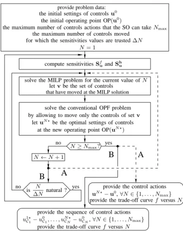
Fig. 3 shows the flowchart of the algorithm of the proposed approaches, which applies in both emergency and normal states, and synthesizes the content of sections IV and V.
The performances of the proposed approaches depend on the accuracy5 of the sensitivities Sfu and S
h
u. It is known that the validity of sensitivities is theoretically ensured only for a small variation of a control around its initial value; hence the validity of sensitivities may not hold true anymore for large excursions of a control or when many controls vary simultaneously. Furthermore, some sensitivities behave rather linearly (e.g. the sensitivity of a branch current with respect to active power injections) while others behave comparatively less linearly (e.g. the sensitivity of a bus voltage with respect to reactive power injections). To let the user the choice about how often it wishes to recompute sensitivities as the operating point changes, we distinguish among two variants of the algorithm.
Variant A: the initial operating point OP(u0) and the sensitivities Sfu and S
h
u are never updated during iterations.
5what matters is rather the relative values of controls sensitivities than their absolute values
that have moved at the MILP solution provide problem data:
no
B
noB
yes yesA
A
provide the sequence of control actions
is N
∆N natural ?
N≥ Nmax?
N← N + 1
let v be the set of controls
solve the MILP problem for the current value of N
compute sensitivities Sf
uand S
h u
for which the sensitivities values are trusted∆N
the initial settings of controls u0
the initial operating point OP(u0
) the maximum number of controls moved
the maximum number of controls actions that the SO can take Nmax
N= 1
provide the trade-off curve f versus N
provide the trade-off curve f versus N uN ⋆− u0 ,∀N ∈ {1, . . . , Nmax} u1⋆ C1− u 0 C1, . . . , uN ⋆CN− u 0 CN,∀N ∈ {1, . . . , Nmax}
let uN ⋆be the optimal settings of controls
by allowing to move only the controls of set v
at the new operating point OP(uN ⋆
) solve the conventional OPF problem
provide the control actions
Fig. 3. Flowchart of the algorithm of the proposed approaches
Consequently, the subset of controls v that moved in the MILP for a given value of N is determined independently of the subsets of controls corresponding to previous values ofN .
Variant B: the initial operating point OP(u0) and the sensitivities Sf
u and S h
u are recomputed to take advantage of the knowledge about the new system state. The update is performed according to the value taken by the parameter∆N which represents the maximum number of controls allowed to move for which the sensitivities values are trusted. The update takes place when the ratio ∆NN takes natural values (e.g. if Nmax = 10 and ∆N = 3 sensitivities are updated for the values ofN ∈ {3, 6, 9}). Clearly, the subset of controls v that moved for a given value ofN includes the subsets of controls corresponding to all values smaller thanN , and identifies only the best next controls to use. The controls corresponding to the previous values of N are free to vary in the MILP and OPF and hence their values may change to take advantage of the new system state (see Section IV-B).
Note that in variant A the solution of the OPF-LNC problem for a given value of N (e.g. N = Nmax) requires only one iteration of this algorithm, while in variant B the OPF-LNC problem is sequentially solved by increasing the value of N from 1 toNmax. Furthermore, only variant A can easily benefit from parallel computations (e.g. the OPF-LNC problems for various values of N being dispatched over the available processors). Thus variant A is expected to perform faster than variant B. On the other hand, only variant B can provide the sequence of control actions u1⋆
C1 − u0C1, . . . , u N ⋆ CN − u
0 CN,
TABLE I
TEST SYSTEMS SUMMARY
system n g c b l t o s
Nordic32 60 23 22 81 57 31 4 12
IEEE118 118 54 91 186 175 11 9 14
618-bus 618 72 352 1057 810 247 175 25
objective value. Variant A provides the volume of control actions to take i.e. uN ⋆− u0,∀N ∈ {1, . . . , Nmax} (vectors
uN ⋆ and u
0 differ by N components) and leaves it to the SO to choose the order of their implementation. The choice of the most appropriate variant for a given application is thus influenced by amount of time within which the user needs to get the solution of the OPF-LNC problem for a given value of N (generally N = Nmax), and/or the trade-off curvef versus
N , and/or the sequence of control actions.
As regards the solution of the OPF-MNC problem it requires only one iteration as variant A.
VII. NUMERICAL RESULTS A. Description of the test systems
We present results obtained with the proposed approaches on three test systems: a 60-bus system, which is a modified variant of the Nordic32 system [16], the IEEE118 bus system [17], and a 618-bus system which is a modified older planning model of the RTE (the French transmission SO) system.
Table I provides a summary of these systems characteristics, wheren, g, c, b, l, t, o, and s, denote respectively the number of buses, generators, loads, branches, lines, all transformers, transformers with controllable ratio, and shunt devices.
The OPF data of the 60-bus and IEEE118-bus systems used in this paper, as well as the relevant numerical results obtained with the various approaches under study, have been archived and made publicly available for comparison purposes [18].
B. Reducing the active power losses
In this section we consider the system operating in a normal state and that the SO’ goal is to minimize the active power losses by acting on generator terminal voltages, LTCs transformer ratios, and shunt reactive power injections. We assume that up toNmax= 10 control actions may be used.
1) Results using the Nordic32 system: The initial value of the power losses is 150.53 MW. The optimal value of the power losses obtained at the solution of the conventional OPF which uses the 39 control variables is 136.64 MW.
Figure 4 plots the value of the objective function in both variants A and B for increasing values of N , while Table II provides the set of controls allowed to move in the conven-tional OPF, where e.g. the control S4046 denotes the shunt connected at bus 4046 while the control Vg13 denotes the voltage of generator g13 (see [16]).
Note that in variant B we consider∆N = 1 (i.e. one control action is taken at the time) and hence the sequence of control actions is provided as a by-product.
Figure 4 shows that variant B provides better solutions than variant A for most values of N (e.g. for N ∈ {3, 7, 8, 9, 10}
144 145 146 147 148 149 150 151 0 1 2 3 4 5 6 7 8 9 10
active power losses (MW)
number of controls allowed to move N variant A variant B
Fig. 4. Nordic32 system: active power losses (MW) versus the number of controls allowed to move N for both variants A and B
TABLE II
NORDIC32SYSTEM:THE SETS OF CONTROLS ALLOWED TO MOVE FOR
INCREASING VALUES OFNFOR BOTH VARIANTSAANDB
N = variant A variant B 1 S4046 S4046 2 S4046, S4071 S4071 3 S4041, S4043, Vg13 Vg11 4 S4041, S4043, S4041, S4046 S1041 5 S4041, S4043, S4041, S4046, S4071 S4043 6 S1041, S4043, S4046, S4071, Vg11, Vg13 Vg13 7 S1041, S1043, S4043, S4046, S4071, Vg12, Vg14 S1011 8 S1041, S1043, S1044, S4043, S4046, Vg9 S4071, Vg13, Vg14 9 S1041, S1043, S1044, S4043, S4046, S1044 S4071, Vg11, Vg12, Vg14 10 S1011, S1041, S1043, S1044, S4043, Vg2 S4046, S4071, Vg9, Vg13, Vg14
while for N ∈ {1, 2, 4, 6} both variants provide the same results). Furthermore, only variant B ensures the objective decrease during iterations. This is because in variant B at each iteration a new control is added to the existing set of controls, while in variant A some elements of the set of controls may disappear for higher values ofN (see Table II). The objective increase observed in variant A for some values of N ∈ {7, 8, 10} indicates that after a certain value of N the sensitivities are not valid anymore, which is due to the significant number of controls moved, the large amount of controls changes, and the nonlinear behavior of the reactive power dispatch problem.
2) Results using the 618-bus system: The initial value of the power losses is 893.81 MW. The optimal value of the power losses obtained at the solution of the conventional OPF which uses the 173 control variables is 866.08 MW.
Figure 5 plots the value of the objective function in both variants A and B for increasing values ofN .
By looking closely at Figs. 4 and 5 one can conclude that variant B leads overall to better objective values than variant A for problems of reactive power redispatch.
C. Removing thermal overloads
We assume that the SO goal in an emergency state in-duced by a thermal overload is to minimize the cost of load curtailment, and that the overload has to be removed very quickly thus preventing the use of cheaper but slower gener-ation rescheduling. We thus consider load curtailment only as
887 888 889 890 891 892 893 894 0 1 2 3 4 5 6 7 8 9 10
active power losses (MW)
number of controls allowed to move N variant A variant B
Fig. 5. 618-bus system: active power losses (MW) versus the number of controls allowed to move N for both variants A and B
120 130 140 150 160 170 180 4 5 6 7 8 9 10 11 12 13 14 15 16 17
OPF objective (monetary unit)
number of controls allowed to move N variant A variant B
Fig. 6. IEEE118 system: objective function versus the number of controls allowed to move N for both variants A and B
control variable, and assume that the allowed percentage of load curtailment at each bus is 10 % of the bus load and is performed under constant power factor. We again assume that the SO is able to take up toNmax= 10 control actions.
Results using the Nordic32 system can be found in [11]. 1) Results using the IEEE118 system: We consider a con-tingency which leads to the overload of a line with 11%.
We solve the conventional OPF and notice that the objective is 118.6 monetary unit, 93.5 MWs are curtailed and Nc =
12 (out of 91) loads share the effort of overload removal. However, in this problem the minimum number of control actions needed to clear the overload isNmin= 4.
Note that because in this case Nc > Nmax, in order to assess the degree of sub-optimality of the computed solution we have performed our approach also beyond Nmax = 10 until the objective of the conventional OPF is attained.
Figure 6 plots the values of the objective function in variants A and B for increasing values of N , starting with Nmin= 4 and up to N = 17. Variant A provides overall better objective values, and as expected, especially for small N , due to the quite linear nature of the active power dispatch problem.
The solution proposed by variant B (resp. A) forN = Nc=
12 is 5.3 % (resp. 10.3 %) larger than that provided with the conventional OPF. We consider that variant B provides an acceptable sub-optimal solution. Observe that in order to identify the 12 controls which move in conventional OPF both variants need to include 17 controls.
Performing the proposed approaches for larger values ofN
155 160 165 170 175 180 185 190 6 7 8 9 10
OPF objective (monetary unit)
number of controls allowed to move N variant A variant B
Fig. 7. 618-bus system: objective function versus the number of controls allowed to move N for both variants A and B
allowed us to encounter some limitations of these approaches which are due to the limited validity of sensitivities:
• the set of controls proposed by MILP does not change as
N increases (especially for some large values of N );
• the conventional OPF is infeasible for the set of controls proposed by MILP (e.g. forN ∈ {11, 12} in variant A);
• the new control proposed by MILP asN increases does not move at the conventional OPF solution (e.g. forN = 14 in variant B and N = 16 in variant A).
Fortunately there exist remedies to overcome these drawbacks, e.g. re-solving the MILP by artificially increasing the over-loads so as to force new controls to move, or by reducing the range of those controls moved in the conventional OPF. We have also noticed that such drawbacks appear less often in variant B, suggesting that it is more reliable than variant A.
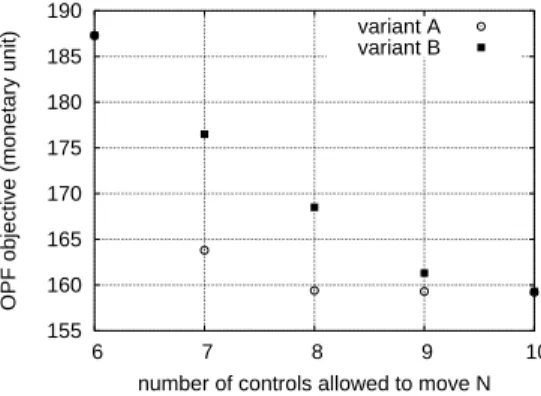
2) Results using the 618-bus system: We consider a con-tingency which leads to the overload of a line with 3.5 %.
We solve the conventional OPF and notice that the objective is 158.3 monetary units, 139.5 MWs are shed, and Nc = 11 (out of 352) loads share the effort of overload removal.
In this case the minimum number of control actions needed to clear the overload isNmin= 6.
Figure 7 plots the value of the objective function in variants A and B for various values ofN , starting with Nmin= 6 and up toNmax= 10. Observe that variant A provides again better objective values. Note also that, in variant A the objective value is very flat for N ∈ [8 10] and only 0.006% larger than the objective of conventional OPF (where 11 controls are used) and therefore, the proposed approaches lead to an excellent near-optimal solution. This figure emphasizes also the importance of SO decision making based on the trade-off curve between the objective and the number of control actions. The analysis of figures 6 and 7 allows to conclude that variant A provides overall better objective values than variant B for active power flows re-dispatch.
D. Removing voltage limit violations
We consider that following a contingency the Nordic32 system operates in an emergency state in which five bus voltages are under their minimum limit (0.95 pu), the total violation of voltage limits at these buses being of 0.102 pu.
TABLE III
THE MINIMUM TOTAL AMOUNT OF VOLTAGE LIMITS VIOLATION AND THE
CONTROL ACTIONS FOR INCREASING VALUES OFN
N = objective (pu) amount of additional control action
variants A and B 0 0.102 -1 0.031 S1041 + 150 MVar 2 0.010 Vg14 + 0.040 pu 3 0.002 Vg11 - 0.046 pu 4 0.000 Vg9 + 0.005 pu 0.9 0.91 0.92 0.93 0.94 0.95 0.96 0.97 0.98 0.99 1 1.01 1.02 1.03 1.04 1.05 1.06 1 2 3 4 5 6
voltage magnitude (pu)
bus number
no control action S1041 + 150 MVar Vg14 + 0.040 pu Vg11 - 0.046 pu
Fig. 8. Evolution of the voltage at some critical buses after taking successive control actions
We assume that the SO’ objective is to find the minimum amount of voltage limit violations given the maximum number of control actions that it can takeNmax. We consider that the set of control actions comprises: generators terminal voltage, LTCs transformers ratio, and shunts reactive power injection. In this case the minimum number of control actions needed to remove the voltage limits violation obtained by solving the MILP approximation of the OPF-MNC problem isNmin= 4. We further assume thatNmax≥ Nmin and solve the MILP approximation (42)-(47) of the OPF-LNC problem for all values of N ≤ Nmin. Table III yields the value of the SO’ objective function and the control actions for increasing values of N . The sequence of proposed control actions consists of: increasing the reactive power of shunt S1041, increasing the voltage of generator g14, decreasing the voltage of generator g11, and increasing the voltage of generators g9.
Note that, due to the small total number of control actions used, both variants A and B (with∆N = 1) provide the same sequence and amount of control actions.
Fig. 8 shows the evolution of voltages at the buses where voltage limits are violated during the sequential implementa-tion of the first three control acimplementa-tions proposed by our approach (due to the small impact on voltages of the last control action in Table III its corresponding curve has not been shown).
E. Computational issues
The CPU times reported hereafter have been obtained on a PC 1.7-GHz Pentium IV with 512-Mb RAM.
In all our trials we have solved the conventional OPF problems by the OPF program [19], which uses the interior point method, and we have solved the MILP problems by the GLPK-v4.35 tool [20], which uses a branch and cut algorithm.
0 200 400 600 800 1000 1200 1 2 3 4 5 6 7 8 9 10 CPU time (s)
number of controls allowed to move N variant A (5 processors) variant A (4 processors) variant A (3 processors) variant A (2 processors) variant A (1 processor) variant B
Fig. 9. 618-bus system: CPU times versus the number of controls allowed to move N for variants A and B
The CPU times of our approaches on the Nordic32 and IEEE118 systems are very small6 and hence do not allow
drawing general conclusions. We therefore limit the analysis of CPU times to the 618-bus system and the active power losses reduction problem.
Figure 9 reports the CPU times of variants A and B for increasing values of N . In variant A, we have estimated the reduction of the CPU time expected by using several processors. We notice that the CPU time provided by variant A cannot be improved by using more than[N/2] + 1 processors. Note that the computational time required by variant B varies rather linearly withN while in variant A it grows more than linearly with N . Furthermore, for N ∈ [4; 10] the best CPU times in variant A are much larger than in variant B.
As expected, we notice that the major computational effort in both approaches is required for the solution of MILP prob-lem7, while the other tasks require comparatively negligible
computational effort (e.g. the computation of sensitivities takes around 0.2 s, the solution of the conventional OPF takes 1.8 s when using all 173 control variables and 1.2 s when using up to 10 control variables only).
On the other hand we notice that, although the MILP problem of thermal overload removal8 (see section VII-C2) has a comparable size with that of reducing the power losses9 it requires much less computational effort (e.g. the former problem takes in average 0.4 s ∀N ∈ [6; 10] while the latter takes 275.2 s for N = 10). The huge difference between the CPU times is due to the larger difficulty of solving the MILP problem of reducing power losses (e.g. many voltage limits constraints are binding or near their limit, many controls have a close impact on the power losses, etc.).
Clearly the reported CPU times can be considerably reduced by: the use of faster MILP solvers, the use of much faster
6The conventional OPF to minimize active power losses for the Nordic32 (resp. IEEE118) system takes 0.1 s and 0.3 s, while the MILP problem for the Nordic32 (resp. IEEE118) system takes 0.2 s and 0.5 s.
7The MILP problem is always solved to optimality.
8This MILP problem comprises 1516 constraints and 704 variables (352 continuous and 352 binary)
9This MILP problem comprises 1583 constraints and 346 variables (173 continuous and 173 binary)
computers, simplifying further of the MILP problem (e.g. by removing harmless inequality constraints and control variables with small sensitivities or a too narrow range), stopping the MILP solution earlier (e.g. as soon as the integrality gap becomes acceptable or when the maximum running time is reached) yielding possibly a sub-optimal set of controls.
We therefore conclude that the computational times of the proposed approaches are compatible with the real-time operation requirements, even in variant A for the power losses reduction problem and for large values ofN .
VIII. CONCLUSIONS AND FUTURE WORKS
This paper has proposed new formulations and solution approaches to the following open questions in the field of OPF computations: the limitation of the number of controls actions to a pre-specified value, the evaluation of the trade-off between the objective function and the number of control actions used, the computation of the minimum number of control actions needed to remove violated limits, and the determination of the sequence of control actions that the SO can take in order to reach its operation goal.
We have shown the interest of our approaches by consider-ing three essential problems for SOs in operational plannconsider-ing and in real-time operation, namely the removal of thermal con-gestions, the removal of voltage violations, and the reduction of active power losses.
The proposed approaches possess several similarities; in particular they combine first order sensitivities, sensitivity-based MILP, and conventional OPF.
We have compared two variants of these approaches depend-ing on whether sensitivities are updated or not and concluded that, in terms of objective value, variant A is better suited for the dispatch of active powers while variant B is better for the dispatch of reactive powers. The sequence of control actions is provided as a by-product in variant B.
We have discussed some possible limitations of our ap-proaches and proposed adequate remedies to overcome them. The proposed approaches are compatible with real-time requirements even for large systems.
Main directions of future works concern:
• the assessment of the degree of sub-optimality of the solutions proposed by our approaches with respect to the optimal solutions provided by standard MINLP methods. • the application of these approaches to the even more complex problems stemming from system restorative state10 and system alert state11.
• the inclusion of the constraints limiting the number of controls allowed to move in post-contingency states in a security-constrained optimal power flow [2], [4], [5] so as to render the latter more useful for the SOs.
• the application of these approaches in an emergency state where both current limits and voltage limits are violated.
10where there is a loss of load, e.g. after a partial or total blackout, no constraint is violated and the SO looks for the sequence of loads, generators, and branches connection to the network [15].
11where no constraint is violated in the current state but some constraints will be violated if some postulated contingencies actually occur [2].
REFERENCES
[1] W.F. Tinney, J.M. Bright, K.D. Demaree, B.A. Hughes, “Some deficien-cies in Optimal Power Flow”, IEEE Trans. Power Syst. Vol. 3, No. 2, 1988, pp. 676-683.
[2] B. Stott, O. Alsac, and A.J. Monticelli, “Security analysis and optimiza-tion” (Invited Paper), IEEE Proc., vol. 75, no. 12, 1987, pp. 1623-1644. [3] B. Stott and E. Hobson,“Power system security control calculations using linear programming, Parts I and II”, IEEE Trans. PAS, vol. PAS-97, 1978, pp. 1713-1731.
[4] R. Bacher (Editors: K. Frauendorfer, H. Glavitsch, and R. Bacher), “Power system models, objectives and constraints in optimal power flow calculations” (chapter of the book “Optimization in Planning and Opera-tion of Electric Power Systems”), Physica Verlag (Springer), Heidelberg, Germany, 1993, pp. 217-264.
[5] J.A. Momoh, R.J. Koessler, M.S. Bond, B. Stott, D. Sun, A. Papalex-opoulos, and P. Ristanovic, “Challenges to optimal power flow”, IEEE
Trans. Power Syst. vol. 12, no. 1, 1997, pp. 444-455.
[6] S.A. Soman, K. Parthasarathy, and D. Thukaram, “Curtailed number and reduced controller movement optimization algorithms for real time voltage/reactive power control”, IEEE Trans. Power Syst., vol. 9, no. 4, 1994, pp. 2035-2041.
[7] W.-H. Edwin Liu, and X. Gupa, “Fuzzy constraint enforcement and control action curtailment in an optimal power flow”, IEEE Trans. Power
Syst., vol. 11, no. 2, 1996, pp. 639-645.
[8] F. Capitanescu, W. Rosehart, and L. Wehenkel, “Optimal power flow computations with constraints limiting the number of control actions”,
Power Tech Conference, Bucharest (Romania), 2009.
[9] E.B. Fisher, R.P. O’Neill, and M.C. Ferris, “Optimal transmission switch-ing”, IEEE Trans. Power Syst., vol. 23, no. 3, 2008, pp. 1346-1355. [10] S.A. Blumsack, “Network topologies and transmission investment
un-der electric-industry restructuring”, Ph.D. dissertation, Carnegie Mellon University, 2006.
[11] F. Capitanescu and L. Wehenkel, “Optimal power flow computations with a limited number of controls allowed to move”, IEEE Trans. Power
Syst., vol. 25, no. 1, 2010, pp. 586-587.
[12] Y.-Y. Hong, C.-M. Liao, and T.-G. Lu, “Application of Newton optimal power flow to assessment of VAr control sequences on voltage security: case studies for a practical power system”, Proc. of IEE C: Generation,
Transmission and Distribution, vol. 140, no. 6, 1993, pp. 539-544.
[13] B. Otomega, A. Marinakis, M. Glavic, and T. Van Cutsem, “Emergency alleviation of thermal overloads using model predictive control”, Power
Tech Conference, Lausanne (Switzerland), 2007.
[14] H.W. Dommel and W.F. Tinney, “Optimal power flow solutions”, IEEE
Trans. PAS, vol. PAS-87, no. 10, 1968, pp. 1866-1876.
[15] T.E Dy Liacco, “Real-time computer control of power systems”,
Pro-ceedings of the IEEE, vol. 62, July 1974, pp. 884-891.
[16] CIGRE Task Force 38.02.08, “Long-Term Dynamics, Phase II”, 1995. [17] IEEE118 bus system, available online at http://www.ee.washington.edu,
1996.
[18] OPF data and numerical results of 60-bus and IEEE118-bus systems, available online at http://www.montefiore.ulg.ac.be/∼capitane/, 2010. [19] F. Capitanescu, M. Glavic, D. Ernst, and L. Wehenkel, “Interior-point
based algorithms for the solution of optimal power flow problems”,
Electric Power Syst. Research, vol. 77, no. 5-6, April 2007, pp. 508-517.
[20] GLPK (GNU Linear Programming Kit) solver, available online at: http://www.gnu.org/software/glpk/, 2009.
Florin Capitanescu graduated in Electrical Power Engineering from the
University “Politehnica” of Bucharest in 1997. He obtained the Ph.D. degree from the University of Li`ege in 2003. His main research interests include optimization methods, in particular optimal power flow, and voltage stability.
Louis Wehenkel graduated in Electrical Engineering (Electronics) in 1986 and
received the Ph.D. degree in 1990, both from the University of Li`ege, where he is full Professor of Electrical Engineering and Computer Science. His research interests lie in the fields of stochastic methods for systems and modeling, optimization, machine learning and data mining, with applications in complex systems, in particular large scale power systems planning, operation and control, industrial process control, bioinformatics and computer vision.