(~) 1990 International Federation of Automatic Control
Decision Trees and Transient Stability of
Electric Power Systems*
L. W E H E N K E L t $ and M. P A V E L L A ? §
A general inductive inference method is proposed and applied to the
automatic building o f decision trees for the transient stability assessment o f
power systems. On the basis o f large sets o f simulations, the essential
features o f the method are analysed and illustrated.
Key Words--Artificial intelligence; pattern recognition; decision trees; electric power systems; data reduction and analysis; decision theory; stability; transient stability analysis, sensitivity and control.
Al~lraet--An inductive inference method for the automatic building of decision trees is investigated. Among its various tasks, the splitting and the stop splitting criteria successively applied to the nodes of a grown tree, are found to play a crucial role on its overall shape and performances. The application of this general method to transient stability is systematically explored. Parameters related to the stop splitting criterion, to the learning set and to the tree classes are thus considered, and their influence on the tree features is scrutinized. Evaluation criteria appropriate to assess accuracy are also compared. Various tradeoffs are further examined, such as complexity vs number of classes, or misclassifieation rate vs type of misclassification errors. Possible uses of the trees are also envisaged. Computational issues relating to the building and the use of trees are finally discussed.
1. INTRODUCTION
Trm DECISION TREE m e t h o d o l o g y is n o w a d a y s recognized to be a generally n o n p a r a m e t r i c technique, able to p r o d u c e classifiers in o r d e r to assess new, unseen situations, or to u n c o v e r the mechanisms driving a p r o b l e m ( B r e i m a n
et al.,
1984; F r i e d m a n , 1977; K o n o n e n k oet al.,
1984; Quinlan, 1986). T h e building of a decision tree is based on a learning set (LS), c o m p o s e d of a n u m b e r of states t o g e t h e r with their c o r r e s p o n d - ing known classification. T h e building p r o c e d u r e starts at the top node of the tree with the entire LS, and progresses by recursively creating successor nodes, i.e. by splitting the LS into subsets of increasing classification purity. T h e p r o c e d u r e is s t o p p e d w h e n all the newly created* Received 13 June, 1989; revised 10 January, 1990, received in final form 25 January, 1990. The original version of this paper was not presented at any IFAC meeting. This paper was recommended for publication in revised form by Associate Editor K-E. Arzen under the direction of Editor A. P. Sage.
t Department of Electrical Engineering, University of Liege, Institute Montefiore, B28, B 4000 Liege, Belgium.
:~ Research assistant F.N.R.S.
§Author to whom all correspondence should be addressed.
115
nodes are " t e r m i n a l " ones, containing " p u r e e n o u g h " learning subsets. T h e ways of splitting the successive subsets, and even m o r e of deciding when to stop splitting, are essential to the method. Often, the lack of general, efficient stop splitting m e t h o d s is e v a d e d by m e a n s of alternative procedures, such as first building a very large tree, then pruning it; they generally rely on empirical justifications applicable to particular cases, but without g u a r a n t e e of effectiveness in o t h e r application domains. T o r e m o v e this difficulty, a stop splitting criterion was d e v e l o p e d on the basis of a general statistical hypothesis test ( W e h e n k e l
et al.,
1989a, b). It was designed independently of any specific application, then applied to p o w e r system transient stability.Transient stability in general is c o n c e r n e d with the system ability to withstand severe contin- gencies. A possible m e a s u r e of this is the
critical
clearing time
(CCT), i.e. the m a x i m u m time that a contingency m a y remain without causing the irrevocable loss of machines' synchronism. T o c o m p u t e CCTs o n e m a y either use t i m e - d o m a i n methods, which solve numerically the nonlinear differential equations describing the system motion, or direct m e t h o d s which rely on the Liapunov criterion (Bergen, 1986; R i b b e n s - Pavella and Evans, 1985). O b s e r v e that the C C T is not a p p r o p r i a t e enough for assessing transient stability, in that it carries partly useless and partly incomplete information; indeed, it m e r e l y provides a rather crude " y e s - o r - n o " answer, whereas what really m a t t e r s in practice is to assess "stability m a r g i n s " and, if necessary, to suggest remedial actions ( E P R I Project, 1987). Within the tree m e t h o d o l o g y , h o w e v e r , the C C T provides a handy m e a n s of classifying the states of a LS.The application of the tree methodology to transient stability was initially proposed in Wehenkel et al. (1986, 1987), then developed in Wehenkel et al. (1989a, b). The leading idea is to compress and organize the information about transient stability in the form of decision trees with the twofold objective: to classify new, unseen states, and to uncover the salient parameters driving the transient stability pheno- mena. Note that the foreseen advantages go beyond this objective: indeed, on-line means to compute stability margins and to infer control strategies were also suggested (Wehenkel et al.,
1988; Wehenkel, 1988). The first results obtained in a few practical examples were quite promising. The constructed trees exhibited nice features, notably with respect to accuracy and complexity. However, to make this method fully reliable and effective, a systematic exploration was necessary. This is a main purpose of the present paper.
Particular attention is paid to learning sets, "adequate" for building efficient decision trees; the way of generating their states in simulations and in real-life situations is discussed, and the influence of their number on the tree features is examined.
Another key issue concerns the splitting criterion. In Wehenkel et al. (1986, 1987), this consisted of a test applied to various "candidate attributes", chosen among static parameters of the power system, a priori likely to drive transient stability. Their influence on the tree structure is investigated below.
The cornerstone of the method is probably the stop splitting criterion (Wehenkel et al.,
1989a, b). Applied to transient stability, this criterion yielded simple, quite accurate trees in the few cases considered so far. In this paper, we determine its optimal parameters, and explore the accuracy and the complexity of the resulting trees.
The number of stability classes to be considered in the automatic building of trees is another question worth considering. Complexity, accuracy, misclassification rate and severity of misclassification errors are all interrelated features. Our purpose is to assess them, and to suggest possible practical applications, not necessarily to decide on a solution.
To conduct the above investigations we need appropriate tools for evaluating trees' accuracy. One of our first concerns will be to consider and compare a priori interesting evaluation criteria.
The ultimate goal for building trees is to use them. This topic is a whole research of its own. In this paper, we will merely indicate possible types of applications.
2. FUNDAMENTALS OF THE METHOD
2.1. General f r a m e w o r k a n d basic notation
The automatic building of decision trees by the proposed inductive inference method implies the existence of a learning set, i.e. of a number, say N, of preclassified states. Without loss of generality, we will assume that each state is characterized by a certain number, say n, of ordered numerical attributes (the same number for each state), and that the N states are classified into two classes only { + , - } . The generalization to more than two-class classi- fications will be considered in Section 2.10; the extension to categorical attributes in addition
to the ordered ones would be quite
straightforward.
In the sequel, a learning set (LS) will be defined by:
t S ~
{(Vl, c1) , (v2, c2) . . . (VN,CN) }
(1) where the components of vector v~Vk = (Vl,, Vzk . . . . , V , , ) r (2) represent the attribute values of the state Sk, which is characterized by its n attributes:
s , = [a, = Vlk] n [a2 = Vzk] n . - . n [a. = v . k l ,
(3)
and whereCk e { +, - }. (4)
Note that the preclassified learning set is considered to be a statistical sample of size N, drawn from the population of possible states.
The test set (TS), is defined as a similar, but independent sample of size M:
TS a___ {(VN+I ' CN+I), (VN+2, CN+2 ) . . .
(vN+,,, ON+M)}. (5)
It will be used for the purpose of evaluating the performance of a decision tree with respect to unseen states (see Section 2.8).2.2. Decision trees ( D T s )
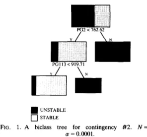
A DT is a tree structured upside down. It is composed of test and terminal nodes, starting at the top n o d e (or root) and progressing down to the terminal ones. Each test node is associated with a test on the attribute values o f the states, to each possible outcome of which corresponds a successor node. The terminal nodes carry the information required to classify the states. Such a DT is portrayed in Fig. 1, built for an example treated in Section 4 in the context of transient stability. Note that in this case, where only numerical attributes are considered, the tests are dichotomic, and the resulting D T is binary: each test node is split into two successors.
PG2 < 762.62
PG113 <919.71
m
m
UNSTABLE --]STABLEFIG. 1. A biclass tree for contingency # 2 . N = 5 0 0 , cr = 0.0001.
A convenient way to define a D T is to describe the way it is used for classifying a state of a priori unknown classification on the basis of its known attributes. This classification is achieved by applying sequentially the test at the test nodes, beginning at the root of the tree, and systematically passing the state to the successor appropriate to the outcome of the test, until a terminal node is finally reached; the state is classified accordingly.
The above description provides an interesting, geometric interpretation of a tree procedure (Breiman et al., 1984): it recursively partitions the attribute space into hyperboxes, such that the population within each box becomes more and more class homogeneous. This in turn allows one to view the classification of a tree as the partitioning of this hyperspace into two regions, corresponding to the two classes. Each class is composed of the union of the elementary boxes corresponding to its terminal nodes. Figure 2 illustrates the geometric representation of the tree of Fig. 1. (Actually, according to this tree structure, the states belonging to the region labelled "stable" have a small chance (13%) to be unstable.)
2.3. Automatic construction o f D Ts
For a given LS, our purpose is to build a near optimal DT, in the sense that it realizes a good tradeoff between complexity and accuracy, i.e. between total number of nodes and classification
J PG2(MW)
1000-
763' ' " OPn ~/0
STABLE
~ PG113(MW~)
920 1000 FIG. 2. Geometric representation of the tree of Fig. 1.ability. Usual ways of estimating accuracy are specified in Section 2.8; anticipating, observe that, intuitively, assessing trees' ability to correctly classify states should rely on test states rather than on states belonging to LS itself.
The ultimate objective of the building procedure is to: (i) select the relevant attributes among the candidate ones (generally the number of retained attributes is much lower than n, the total number of candidate attributes); (ii) build the decision tree on the basis of these relevant attributes. This building procedure is described below (Wehenkel et al., 1989a).
• Starting at the root of the tree, with the list of candidate attributes and with the whole LS, the learning states are analysed in order to select a test which allows a maximum increase in purity or, equivalently, which provides a maximum amount of information about their classification. The selection proceeds in two steps:
(i) for each attribute, say ai, it finds the optimal test on its values, by scanning the values of this candidate attribute for the different learning states; in our case of ordered numerical attributes, this step provides an optimal threshold value vi. and defines the test
a i < v i , ? (6) (ii) among the different candidate attributes, it chooses the best one, a , , along with its optimal value, v**, to split the'node. In short, step (ii) defines the optimal attribute, step (i) its optimal threshold value.
• The selected test is applied to the learning set of the node and splits it into two subsets, corresponding to the two successors of the node. Starting with the root of the tree and the entire LS, the two subsets
LS1 & {Vk e LS I a . < v**} LSz ___a {Vk e LS I a . --> v**},
correspond to the two successors of the root. • The successors are labeled terminal or not on
the basis of the stop splitting criterion described below.
• For the nonterminal nodes, the overall procedure is called recursively in order to build the corresponding subtrees.
• For the terminal nodes, the class probabilities p+ and p_ are estimated on the basis of the corresponding subset of learning states there stored, and the class label of the majority class is attached.
Obviously, the crux of the entire construction of a D T lies in the selection of the splits and the
of a DT lies in the selection of the splits and the decision whether to declare a node terminal or to continue splitting. These two questions are examined below, after the introduction of some necessary notions of (im)purity and information, drawn from the information theory.
2.4.
Mathematical formulation
2.4.1.
Definitions.
Denoting by:S the subset of all possible states, correspond- ing to some node of a DT, i.e. directed to that node by the classification procedure;
p ( + IS) (resp. p ( - IS)) the probability of a random state drawn from S to belong to the class + (resp. - ) ;
T a dichotomic (candidate) test [e.g. see (6)] on some attribute's values of the states;
Sy (resp. S,) the subsets of S of states yielding the answer "YES" (resp. "NO") to the test T; these sets would correspond to the successors of the node split on the basis of T;
p(Sy IS ) (resp. p(S, IS)) the probabilities of the outcomes "YES" and "NO" in S; one defines the following measures.
The
prior
"classification entropy" of SHc(S) & - [ p ( + I S) log2 ( p ( + I S))
+ p ( - IS) l o g 2 ( p ( - I S))]. (7) Hc(S) is a measure of the impurity or the uncertainty of the classification of a state of S; H e ( S ) = 0 corresponds to a perfectly pure ( p ( + ] S ) = 1 or 0) subset, whereas H c ( S ) = 1 corresponds to p ( + IS) = p ( - I S) = ½, i.e. max- imal uncertainty.
The entropy of S with respect to the test T Hr(S) & -[p(Sy I S) log2 (p(Sv I S))
+ p ( S , I S)logz(p(S, Is))]. (g) Hr(S) is a measure of the uncertainty of the outcome of T in S; with respect to the outcome of T, it has similar properties to Hc with respect to the classification.
The mean
posterior
"classification entropy" of S given the outcome of THc,r(S) a--p(Sy I S)Hc(Sy)
+ p ( S , I S)He(S,). (9)Hclr(S)
is a measure of the residual impurity if Sis split into Sy and S~ according to the outcomes of test T.
The "information" provided by T on the classification of S
IV(S) & Hc(S) - Hc,T(S); (10)
IV(S) is a measure of the ability of T to produce pure successors.
The normalized information gain of T
Ccr(S) & 21~(S) (11)
He(S) + Hr(S) "
Remark.
The measures defined in (7)-(10) areexpressed in bits whereas that in (11) is dimensionless.
2.4.2.
Interpretation.
It is possible to give a qualitative interpretation of the relation between ccT(s) and the classification ability of the test T. To this, first observe that the following inequalities can be easily shown:0 < Hc(S), HT(S),
HCIT(S ),
I~(S), Ccr(S) - 1(12)
Hc,T(S), I (S) <-- He(S).
(13)
Then consider the two following extreme cases:1. The outcome {"YES", "NO"} of T and the classification {+, - } are statistically inde- pendent, i.e. the test T provides no information at all about the classification. In this case p ( + I S y ) = p ( + ] S , ) = p ( + IS) and
p ( - [ S y ) = p ( - ] S , ) = p ( - I S ) . (14) Thus, Hc(Sy) = Hc(S,) = Hc(S) and according to
(9),
Hcir(S)=
Hc(S). In addition, by virtue of(10) and (11),
i (s) = c (s) = o.
2. The outcome of T provides pure classified subsets Sy and S,. Then necessarily Hc(Sy)= Hc(S,) = 0. According to (9), this implies that Hclr(S) = 0 and IcT(s) =Hc(S). Moreover, in
this case the probability
p(Sy
IS) (resp.p(S, IS)) will be equal to either p ( + IS) (resp. p ( - IS)) or p ( - IS) (resp. p ( + IS)), and thus Hr(S) = Hc(S) and
C~(S) = 1.
From the above it follows that the higher the value of cV(s), the more interesting the test T for splitting the node corresponding to S. This is exploited in Section 2.5 to define the optimal splitting rule, used in the building of DTs.
2.4.3.
Estimation on the basis of the sample
of learning states.
The information and entropymeasures defined in (7)-(11) cannot be comp- uted directly since the probabilities involved are generally unknown. Therefore, we use the learning set as a statistical sample and estimate the probabilities by their empirical values computed in the LS. More precisely, the set S, corresponding to some node of the DT, is
replaced by the
subset
of learning states (i.e.SNLS) corresponding to this node. The
computation of p ( + IS), p ( - IS),
p(Sy
IS) and
p(S~ IS) of this subset is then straightforward, since the classification and attribute values of the learning states are known.It should be noted that, although the estimates of p ( + IS), p ( - IS),
p(Sy
IS) and p(S, IS) aregenerally unbiased, their substitution in (7)-(11) provides rather optimistically biased information measures, thus overestimating the actual "good- ness" of the test T. Fortunately, the amount of bias is inversely proportional to the sample size (the number l of states in S O L S ) and the measures may still be used for comparison purposes, e.g. in order to select an "optimal" test for splitting the node.
For example, it can be shown (Kv~lseth, 1987) that for an actual value of I ~ ( S ) = 0 (no correlation), its estimate
i = t~(S n LS) (15)
has a x-square like distribution, the expectation (or bias) of which is positive and inversely proportional to the number l of states in S n LS. This property is exploited below, in the stop splitting criterion.
In the sequel, to emphasize the difference between the purity measures and their estimates, we will call the latter "apparent" as opposed to the "real" unknown values.
2.5. On the optimal splitting criterion
Obviously, the splits at the test nodes should be selected so as to avoid to the extent possible the appearing of deadends (i.e. of impure terminal nodes, see the definition given below in Section 2.6), and to obtain the desired degree of accuracy. This is done in a more or less heuristic (not necessarily optimal) fashion: the best test (defined by the optimal attribute together with its optimal threshold value, see Section 2.3), is considered to be the one which separates at most the states of the two classes in the local learning subset. This strategy amounts to selecting the split which yields the purest direct successors, or maximizes the apparent normalized information gain C~(S n LS) defined in (11). In that sense, it may be considered to be locally, rather than
globally optimal.
2.6. Stop splitting method
Many methods were proposed. For example, ID3 (Quinlan, 1986) stops splitting at a node only if the corresponding learning subset is completely included in one of the classes of the goal partition. Unluckily, in many situations, as shown by our experience, this strategy tends to build overly complex DTs, most of the terminal nodes of which contain only a very small and unrepresentative sample of learning states. They perform generally badly with respect to unseen situations and are unable to indicate in a reliable way the inherent relationship between the attributes and the goal classification. To circumvent this difficulty we propose a more
conservative criterion, which stops splitting a node if one of the following two conditions is met:
1. The local subset of learning states is sufficiently class pure. Such a terminal node will be called a leaf in the sequel. The degree of class purity required for leaves is a parameter of the algorithm and fixes the amount of detail we want the DT to express.
Note. Actually, the degree of residual "im-
purity" may be specified by Hm, the maximal residual entropy [see (7)]. The entropy of the learning subset relative to a node, is inversely proportional to its purity. Thus, in terms of entropy, a node will be a leaf only if its entropy is lower than Hm. In the practical investigations reported in this paper, a constant value of Hm=0.1 bits was used. This very low value amounts to building DTs as detailed as possible. Higher values could be of interest if one wanted to build simpler "first guess" DTs, for data exploration purposes.
2. There is no possibility to enhance the DT accuracy in a statistically significant way by splitting this node further. In other words, given the optimal dichotomic split for this node, there is not enough evidence in the local learning subset, that this split would actually improve the real performance of the DT. Such a terminal node is called a deadend in the sequel. This second criterion prevents the building of unnecessarily complex DTs. It is formulated as a statistical hypothesis test:
Given the local subset o f learning states and the optimal split, can we accept the hypothesis that the apparent* increase in accuracy, as measured in this subset, provided by the split, is a purely random effect?
In quantitative terms, the statistic ~ a--cli
(where I is the size of the local learning subset, c a constant and t the apparent increase in purity provided by the optimal split) is distributed according to a x-square law (with one degree of freedom) under the hypothesis of no real
increase in purity. Hence, if we fix the a~-risk of not detecting these situations to a given value, testing the value of ,/i against the threshold -4or such that Prob(fi~---fi~cr)= a~ allows one to detect the cases where the apparent increase in accuracy is a random effect, with a probability of 1 - a~. Figure 3 sketches such x-square probabil- ity density functions.
* Apparent as opposed to real increase in accuracy, means the increase measured in the LS as opposed to the increase measured for unseen states.
~ f . . . 3 degrees of [reedom
FIG. 3. ;c-square probability density functions of ,4.
Thus, the or-risk of the hypothesis test fixes the amount of evidence we require at each node in order to split it; the answer depends on the value of or, the size of the local learning set, and the amount of apparent accuracy improvement provided by the test. The question of " h o w much evidence should be required to allow the splitting of a node", is related to the degree of representativity we impute to the learning set and the risk that this degree is overestimated. Therefore, the degree of cautiousness of the procedure is fixed by the user via the selection of the value of or. This value ranges from 1 (the criterion has no effect on the splitting procedure anymore, and the tree grows according to the above condition 1) to zero (no growth is allowed, the tree reduces to its root).
The value of cr has indeed drastic effects on the resulting trees characteristics as illustrated by the following example (borrowed from Section 4, below). Four DTs were grown for o~ assuming the values 1.0, 0.1, 0.01 and 0.0001; they were built on the basis of a LS composed of 500 states and evaluated on the basis of an independent test set of 1500 other states. Table 1 reports their complexity and accuracy, i.e. the number of their nodes and the percentage of correctly classified test states. These quite impressive figures illustrate that the larger trees are less accurate than the smaller ones and on the other hand that the appropriate selection of cr allows the building of small, yet better DTs (see also the discussion of Section 2.9 and the simulation results of Section 4.3.2).
2.7.
Comparison with the ID3 method
The proposed inductive inference method originates from the ID3 algorithm, from which, however, it departs in some essential respects.
TABLE l
¢r 1.00 0.1 0.01 0.0001
Complexity 63 55 7 5
Accuracy 88.1 88.5 91.2 91.2
Below, we collect the main differences between the two methods.
Application domain.
ID3 was initially in-tended to handle mainly
symbolic
anddeterministic
learning problems characterized byvery large (almost complete) learning sets composed of objects described by discrete (or qualitative) attributes only. Thus, it was essentially designed to handle large sets of data, in order to
compress
rather than extrapolate their information (Quinlan, 1984). On the contrary, the proposed method is especiallytuned to handle mainly
numeric
andnondeterministic
problems, where the learningset has to be
generalized
in an appropriate fashion. The method is general enough to handle at the same time numeric and qualitative attributes and can be tuned to the degree of "representativeness" of the learning set, via the appropriate choice of the threshold cr (see Section 4.3 below).Stop splitting criterion.
ID3's stop splittingcriterion amounts to building DTs which classify the learning set as correctly as possible, which is indeed the best approach if the latter is almost complete. The proposed method, on the other hand, stops splitting earlier, as soon as the statistical hypothesis test alows to conclude that
no
significant
improvement of the tree's accuracywould be achieved by developing the node anymore. This is quite different, and enables the method to take the best advantage of learning sets which are only partly representative of the possible objects. This is further discussed in Section 2.9 below.
Optimal splitting criterion.
ID3 considers thebest test to be the one providing the largest apparent information gain i c r. It has been found that this measure is biased in the favour of those having the largest number of succes- sors, especially in the context of randomness (Quinlan, 1986). Note that this is supported by the fact that the number of degrees of freedom of the z-square distribution (and thus its bias) increases linearly with the number of successors of a split. The
normalized
correlation measure Cc T evaluates the tests more objectively since the number of succesors is compensated by the term /4r in its denominator.Strategy.
ID3's strategy, embodied by itsoptimal and stop splitting criteria, amounts to building trees which maximize the
apparent
reliability,
regardless of their complexity. On theother hand, the strategy of the proposed method is to build DTs maximizing a measure of
quality
which realizes a compromise betweenapparent
reliability
andcomplexity.
The latter is moreeffective in the context of incomplete and random data (Wehenkel, 1990).
2.8. Evaluation criteria
The criteria described below (e.g. see Touss- aint, 1974) allow assessing the accuracy of a D T in general, or equivalently, its misclassification rate. Observe that these are only estimates, since in real world problems it is seldom possible to scan all the possible states, even in deterministic type problems.
Resubstitution estimate, R ~S obtained by con- sidering all the states belonging to the LS, dropping them through the D T , and computing the ratio of misclassified over the total n u m b e r (N) of states;
Test sample estimate, R TM obtained by con- sidering all the states belonging to the TS, dropping them through the D T , and computing the ratio of misclassified over the total n u m b e r (M) of states;
Cross-validation estimate, R cv obtained by: (i) dividing the total n u m b e r of learning states into, say V, equally sized subsets, using one of them as the test set and the union of the remaining V - 1 as a learning set; (ii) building a D T based on this learning set and assessing its accuracy on the basis of the test set; (iii) repeating this procedure V times by considering successively each of the V subsets as test set; (iv) taking the average of the V individual estimates as the final accuracy. The validity of the p r o c e d u r e implies that V is quite large ( > 1 0 ) , so that the D T s constructed on the basis of the ( V - 1 ) subsets are (almost) identical with the initial D T , constructed on the basis of the total n u m b e r of states (V subsets). For V = N this is the so-called " l e a v e - o n e - o u t " estimate.
Remark. The above defined measures can be considered as more or less accurate estimates of the true probability of misclassifying a new state. They have the following characteristics.
R ~s is easy to c o m p u t e and requires no additional samples but is generally optimistically biased, underestimating the real probability of error. Intuitively, for fixed N, the larger the D T , the higher the correlation between the D T and the LS, and the more biased R ~.
R t~ is the most reliable and unbiased estimate and is easy to compute. M o r e o v e r , if M is sufficiently large its variance is small. Its main drawback is that it requires additional states in sufficiently large number, which cannot be used in the learning set. A n o t h e r advantage of R ts is that one can easily estimate its variance and therefrom c o m p u t e confidence intervals. In the sequel we will consider this estimate as the benchmark.
R cv combines advantages of the two preceding measures, since it is generally less biased than R ~s and does not require additional states. On the other hand, its variance can be very large, and certainly depends strongly on the charac- teristics of the problem at hand. In practical situations, when the n u m b e r of samples is limited, it is an interesting alternative to R ts. Notice also that the computational burden required for R cv can be very heavy, since it needs the building of V additional DTs.
The above considerations are illustrated in Section 4, on a real world example.
2.9. On the right size of trees
The stop splitting m e t h o d introduces the statistical threshold p a r a m e t e r tr. Varying its value allows to modify the size of a tree. But how to choose the right tree size? The choice should be guided by the observation that too large a D T will yield a higher misclassification rate and hide relevant relationships, whereas too small a tree will not make use of some of the information available in the LS. Indeed, the terminal nodes of a too small D T have not been expanded enough and this prevents from getting the purer subsets and the corresponding insight about the role that the attributes would have played in this expansion; a too large D T , on the other hand, results from the splitting of statistically unrepresentative subsets; therefore, it is likely to cause an increase in the misclassification rate when classifying states not belonging to the LS. Stated otherwise, a tradeoff appears between the two following sources of misclassification: bias (overlooking significant information in the LS) and variance (badly interpreting the randomness in the LS): too large a tree will suffer from variance whereas too small a tree will present bias.
2.10. Building multiclass DTs
The above description of the inductive inference m e t h o d made in the case of two classes { + , - } , is general enough to handle (at least in principle) an arbitrary number, say m of classes, provided that m remains negligible with respect to the size N of the LS.
Indeed, on one hand the information theoretic purity measures defined in (7)-(11) may be generalized to m classes; on the o t h e r hand the statistical hypothesis test remains applicable, provided that m - 1 degrees of f r e e d o m are used (instead of 1 in the two-class (or biclass) case) for the x-square law.
DTs classifying directly the states into one of the m specified classes.
Another indirect possibility would be to build m - 1 biclass DTs and to combine them in order to obtain the m-class classification.
In the investigations of Section 4 we use the first, direct approach. The obtained DTs are simpler and easier to interpret. Moreover, preliminary investigations indicate that they are at least as good, sometimes better, from the accuracy viewpoint, than the indirect multi- biclass trees.
3. DECISION TREE BASED TRANSIENT STABILITY APPROACH
Two main conjectures underlie the application of the tree method to transient stability assessment. First, transient stability is strongly dependent upon the contingency type and location; hence the idea of building a tree per contingency. Second, transient stability is a quite localized phenomenon, and is driven by a few number of the system parameters; hence the idea of proposing candidate attributes selected among the parameters of the system in its steady state condition.
These generally well-accepted conjectures, have also been verified in the few cases treated by the tree methodology (Wehenkel et al.,
1989a, b). The case study of the next section attempts to further validate them by means of exhaustive simulations. It also provides answers to questions raised by the overall decision tree
transient stability (DT-FS) method, whose prin-
ciple is recalled below.
3.1. Principle of the D T T S approach and related questions
This may be formulated as follows: for each preassigned contingency, build up off-line a DT on the basis of a learning set and of candidate attributes. This tree is then used on-line to classify new, unseen states in as many classes as desired; for example, in a biclass tree, a given state would be classified as either stable or unstable, whereas in a three-class tree, the same state would be declared stable, fairly stable, or unstable.
Below, we identify questions relevant to this definition and suggest answers, often anticipating the results of Section 4.
3.1.1. Questions about the LS.
(i) How to obtain the learning states; (ii) How to classify them;
(iii) How many states should be used for the efficient construction of a DT;
(iv) Whether the "right" size of LS should be
dependent upon the size of the power system.
Tentative answers.
(i) Either by considering plausible scenarios and running a load flow program to get the corresponding operating states, or by using past records of the system real life;
(ii) According to their CCT values, computed via a time-domain or a direct method as appropriate;
(iii) This question is explored in the next section;
(iv) The answer to this question is postponed until Section 5.
3.1.2. Questions about the list of candidate attributes.
(i) What kind of candidate attributes to select for test (6);
(ii) How many;
(iii) What would happen if the actually most relevant attribute were for any reason masked, i.e. discarded from the list;
(iv) What if additional relevant attributes are further considered.
Tentative answers.
(i) Parameters of the system in its steady state, pre-contingency, operation;
(ii) When no prior knowledge of the system can guide the selection, it is advisable to consider as many as possible candidates of the type just suggested, confined in a relatively restricted area surrounding the contingency location; note that the increase in computing cost is insignificant (see below);
(iii) It would generally lead to somewhat more complex, yet quite accurate DTs, provided that other relevant attributes are still present in the list;
(iv) See results of Section 4.3.4.
3.1.3. Questions relating to the number of classification patterns.
(i) Which are the main differences between trees of small and large number of classes; (ii) For a given misclassification rate, which type
of trees provides narrower misclassification error.
Tentative answers
(i) One can reasonably conjecture that the smaller the number of classes in a tree, the less complex and more accurate this tree; (ii) Provided that the inductive inference
method is correctly developed, it is normal to think that the larger the number of classes in a tree, the less severe the misclassification
errors; indeed, in a well designed tree, misclassification errors will result in adjacent classes; it is therefore less severe to declare fairly stable a state which actually is stable (three-class tree), than to declare it unstable instead of stable (two-class tree) (see Section 4.3.5).
3.1.4. Questions relating to computational aspects.
(i) Which is the most expensive task of the DTI'S approach;
(ii) How does the number of candidate attributes affect the computing time of a DT;
(iii) How does the number N of learning states affect the computing time of a DT;
(iv) How "expensive" is the storage of DTs; (v) How "expensive" is their use.
Tentative answers.
(i) The generation of a LS is undoubtedly the most demanding task; and the more refined the system modelling, the more expensive the task;
(ii) According to the splitting criterion proce- dure described in Section 2.3, the time required by a DT building varies linearly with the number of candidate attributes; (iii) In terms of the size of the learning set, the
computing time is upper-bounded by--and generally much lower t h a n - - N log N, i.e. the time required to sort the LS according to the values of the n candidate attributes; (iv) The storage of a DT is generally extremely
inexpensive; indeed, it is proportional to the number of its nodes, which is found to be quite small (see next section); to fix ideas, a compiled LISP version of a DT-classifier composed of 25 nodes (which can be considered as an upper bound for the DT'FS method) takes about 600 machine instructions, meaning that in the context of modern computer architectures thousands of DTs can be stored simul- taneously into main memory;
(v) The mean classification time of a state by means of a DT is almost negligible (about 0.6 ms for a DT comprising 25 nodes).
given contingency: considering the appropriate DT, and applying to this state the test (6), one successively directs it through the various nodes of the tree, until reaching a terminal node; the state is classified accordingly. One could object that the information thus obtained is less refined than the CCTs used to classify the states of the LS; this however is not surprising, since the precise CCT values of the learning states are not fully exploited during the tree building. Weh- enkel et al. (1988) and Wehenkel (1988) proposed a means to approximately estimate the CCT of the state one seeks to classify, by using the notion of "distance to a class", whose definition takes into account the CCTs. This distance, inferred from the geometric interpreta- tion of a DT outlined in Section 2.2, is schematically illustrated in Fig. 2. One can see that the operating state (or point, OP) labelled OPn is stable, whereas the state OP1 is unstable and OP2 is very unstable. Moreover, it shows that to (re)inforce stability, one should suitably direct the OP in the attribute space, i.e. suitably modify the values of its relevant attributes.
The above short description suggests that the DTrS approach can provide three types of transient stability assessment: analysis, directly linked to the classification of an OP, sensitivity analysis, linked to the "distance of an OP to a class", and control, linked to the way one can act to modify such a distance. Moreover, since the involved computations are likely to be extremely fast, several real-time strategies may be conceived. For example, one may proceed in a way similar to the standard "contingency evaluation" of steady state security assessment,
viz.: draw up a contingency list, and build
off-line the corresponding DTs; then, in real-time, scan the list, focus on those contingencies which are likely to create prob- lems, and if necessary propose corrective actions. Of course, care should be taken so as to avoid incompatible actions. But for the time being this question is beyond our scope.
Finally, observe that the DTs provide also a clear, straightforward insight into the complex mechanism of transient stability. This is not the least interesting contribution of the DTI'S approach.
3.2. Possible types of uses of the DTs
Various uses can be inferred by following the pattern of the general DT methodology (e.g. see Section 2.2); many others are specific to the DTI'S approach.
The use which immediately comes to mind is the classification of an operating state of a priori
unknown degree of stability with respect to a
4. CASE STUDY
4.1. General description
The investigations conducted in this section aim to answer the questions previously raised, to assess the salient features of the D T r s approach and to test the conjectures underlying it.
The power system we have chosen is small enough to avoid unnecessarily bulky computa-
tions, but large enough to draw realistic conclusions. It is composed of 31 machines, 128 buses and 253 lines; its total generation power in the base case amounts to 39,000MW. This system is described in Lee, (1972), and sketched in Fig. 4. (The rationale of its decomposition is discussed in Section 4.2.1.)
In this first set of large-scale simulations we adopted the standard simplified system modell- ing, i.e. constant electromotive force behind transient reactance for each machine and constant impedance for each load.
To assess the D T T S m e t h o d as objectively as possible, we have generated 2000 operating points (OPs). Two sets of simulations were considered, corresponding to very severe contin- gencies, consisting of three-phase short-circuits (3q~SCs) applied at generator buses (one at a time). The first set concerns thorough investiga- tions carried out with three such stability scenarios, of 3q~SCs applied at buses # 2 , 21, and 49, arbitrarily chosen.* This implied the computation of 6 0 0 0 C C T values. Part of the OPs along with their classification have been used in the LS, the other part composing the TS. A large number of DTs have been built for the above three contingencies, for various sizes of LSs, varying values of the threshold ~r, and three different classification patterns, namely two-, three-, and four-class classifications. In the two-class case, one distinguishes stable and unstable OPs, depending upon whether their CCT is above or below a certain threshold C C T value; in the three-class case one distinguishes stable, fairly stable and unstable OPs (two threshold CCT values are used); in the four-class case one distinguishes very stable, stable, unstable and very unstable OPs (three threshold values). The threshold CCT values are a priori chosen rather arbitrarily, but so as to avoid a too important imbalance between the populations of OPs belonging to the various classes.
The second set of simulations is described in Section 4.4.
4.2. Constitution of a data base
The data base was randomly generated on the basis of plausible scenarios, corresponding to various topologies, load levels, load distributions and generation dispatches. H e r e a f t e r we de- scribe the way used to generate them, to analyse them from the transient stability point of view, and to build the attribute files.
4.2.1. Random generation of OPs. To gen- erate these various states, we grouped the nodes * In the sequel, a contingency will often be specified by merely the number of the generator bus at which it is supposed to apply; e.g. contingency (or fault) ¢t2, #21, ~49.
of the power system into five internal zones, and one external zone composed of the boundary nodes of the system and its external equivalents (Fig. 4). The internal zones were defined empirically, on the basis of the "electrical distances" (number and length of lines) connect- ing their nodes. The OPs composing the data base were generated randomly according to the following independent steps.
1. Topology: it is selected by considering base cases (with probability 0.5) and single outage of a generator, a load or a shunt reactor (each with probability 0.08), a single line (with probability 0.16), two lines (with probability 0.1). The outaged element is selected randomly among all the elements of the power system.
2. Active load level: the total load level is defined according to a Gaussian distribution (with/~ = 32,000 MW and o = 9000 MW). 3. Distribution of the active load: the total load is first distributed among the six zones according to the random selection of participation factors (see below), then among the load buses of each zone homothetically with respect to their base case values. The reactive load of each bus is adjusted according to the local base case power factor. This results in a very strong correlation of the loads of a same zone, and a quite weak one among loads of different zones.
4. Distribution of the active generation: in a similar fashion, the total generation is first distributed among the zones according to randomly selected participation factors, then among the generators of each zone according to a second selection of participation factors. Thus, neighbour generators are less correlated than neighbour loads. The reactive generations are obtained by a load flow calculation. T o avoid overloads, the final active generation of each generator is constrained to 90% of its nominal power.
Note. In order to avoid overloading or under- loading the slack generator, the total generation is defined as the total active load plus a polynomial approximation of the active network losses of form:
Network Losses (MW)
1336 - 255P~ + 19P~ - 0.7P 3
+ 0.012P 4 - 0.00007P 5 where P~ denotes the total active load of the OP, in GW, and where the coefficients were determined by a least squares estimation on the basis of 11 OPs of different load levels for which the network losses were computed by a load flow program.
Io~ 125 ', 67 :::~. .10 -- ' 129 165 - 12t,(~ 1 N' 16 110 " ... r --,;~l ...
[
< 87 88]
31-MACHINE
SYSTEM
3h5 kV 765 kV c:. "l. Towards the o f external zone I 03 83 85 633~ I 50 ,"
°'
I'0,
"
_~_~[-
I]
-j
~'
1321
~,-,,
[ - / JZONE
1
:L
60 lg 78 / ' 1132 11221--,
±
!!~r--'
[
ii
IS~1~73 ' ZS~]L
,~:;7
..,
F ... i 98 I • -,P-t-:
39~_11
:611
I . I I 7--"/.0 I lZ9 I 130 7t, ~S ] '~ 75 27 0 ~5 9t, 0 931~' Z.5 ¢0) "1"55 !e6 91 90 ~ 89 FIG. 4. One-line diagram of the 31-machine test system and its decomposition.5. Load flow calculation: to check the feasibility of an operating point and compute its state vector, it is fed into the load flow program, and accepted if the latter converges properly. (About 90% of the states were accepted.) (Remember that the power system has 128 buses and hence each state vector has 2 × 128 - 1 = 255 components.)
Participation factors. To distribute a given amount of active (generation or load) power (say Ptot) on a number, say E, of "elements" (zones, loads or generators) we use the following procedure.
Let p/N, ( i = 1 . . . E) be the "nominal" power of the elements (for zonal loads we use the base case total load of the zone, for generators their nominal power and for zonal generations the sum of the nominal generations of their generators), and ).~, ( i = 1 . . . E), positive coefficients selected randomly, accord- ing to the procedure described below. The participation of each element is individual
defined by:
ei &-- AieN Ptot. (16)
E
X z,e
j--I
Thus, the ~., coefficients act as a distortion with respect to the homothetic nominal power distribution. They are selected randomly in the following way:
One third of the cases are defined by 2~ i= 1, ( i = 1, . . . , E), i.e. no distortion with respect to the nominal distribution;
The rest of the cases are defined by ~'i = 2, for a randomly selected value of j, and ).i---l, (i = l . . . j - l, j + l . . . E ) , i.e. a higher participation of the j t h element.
4.2.2. Transient stability (pre)analysis and attribute calculation. To use the data base for investigating the DTTS approach, we carried out the following preliminary calculations:
1. Approximate calculation of the CCT of the 2000OPs, for a 3~bSC at each one of the 31 generator buses, using the extended equal area criterion ( E E A C ) (Xue et al., 1988). This gave us good information about the relative severity of these contingencies in relation to the OPs represented in the data base, and allowed us to select three "interesting" ones for our investigations.
2. Precise calculation of the CCTs of the OPs, for the three selected faults, using the step by step (SBS) method. To accelerate the iterative cut and try process delimiting the precise value of the CCT, the approximate values supplied by
the E E A C were used as an initial guess. Incidentally, these latter were found to be in a very good agreement with those computed by the SBS method (over the 6000 CCT values we found a negative bias of -0.007s and a standard deviation of 0.032s of the CCTs provided by the E E A C as compared to those computed by the SBS method).
3. Generation of the files containing the attribute values for the 2000 OPs. About 270 different "primary" attributes have been com- puted, comprising zonal statistics on loads, generation and voltage, voltage magnitudes at all buses, voltage angles at important buses, active and reactive power of each generator, and topology information for each OP. Other attributes, such as line power flows, could be defined as simple algebraic combinations of the primary attributes and did not necessitate to be stored explicitly. The attribute files were constructed on the basis of the load flow data and state vectors.
Overall, the data base contains about 300 values per operating point, in addition to the input files required for the load flow and transient stability analysis programs.
4.3. Simulation results
Over 400 different DTs were built for various scenarios: three different contingencies, about 15 different classifications, distributed almost equally among the two-, three-, and four-class patterns, learning set sizes ranging from 100 to 1500OPs, more than 100 different candidate attributes, cv values ranging from 1.0 to 0.00005. The DTs were evaluated on the basis of independent test sets.
The resulting observations are organized and presented in six parts (Sections 4.3.1-4.3.6), although they are interdependent in many respects. The first part analyses general DT features, such as complexity and accuracy, with respect to various classification patterns, while fixing the other parameters (size of the LS, value of tr, list of candidate attributes); this provides a good insight into the overall DT'FS method. The second part focuses on the influence of cr on the resulting DTs, and suggests how to select good t, values in practical situations. The third part explores the way the size of the LS affects the DTs, while the fourth part discusses the influence of the candidate attributes on the DTs. The fifth part examines the influence of the number of classes on the misclassification rate and severity. Finally, the sixth part compares the different accuracy estimates defined in Section 2.8.
TABLE 2. TREE FEATURES AS RELATED TO THE NUMBER OF CLASSES. ~ = 0.0001, N = 500, M = 1500
Two classes T h r e e classes F o u r classes Gen.
bus # N, RtS(%) A N t R t S ( ° ~ ) A N t Rts(%) A
2 7 2.27 3 17 5.67 4 27 9.60 7
21 9 3.73 3 17 3.60 4 25 8.40 6
49 5 1.53 1 9 4.33 2 15 7.53 3
4.3.1. General tree characteristics. DTs cor- responding to three different classifications patterns (of two, three and four classes) are built for each of the three different contingencies under the following conditions: the data base (2000OPs) is divided in a LS composed of N = 5 0 0 O P s and a test set composed of the M = 1500 remaining OPs (this fairly large size provides a high precision to the R ts estimate); the value of tr is fixed to 0.0001 (the justification of this choice will be found below); and the list of candidate attributes, the same for each DT, is composed of 81 static variables.
The results are summarized in Table 2. The first column specifies the faulted bus number of the contingency. The nine following columns specify for the indicated contingency and number of classes, the characteristics of the resulting DT:Nt, the total number of its nodes (which measures its complexity); R ts, its test sample estimate, representing the percentage of misclassified test states; A, the number of different retained attributes among the 81 candidates. This is repeated for the three contingencies, providing the features of nine DTs listed in the table.
The same set of investigations was repeated three more times, with three other learning sets of the same size (each of 500 states), in order to detect the variability of the DTs with the LS. The obtained results are very similar to the above, and induce the following conclusions: --The complexity increases from the very simple
two-class trees to the moderately complicated three- and four-class ones;
--Their accuracy is quite satisfactory especially in the two- and three-class cases; the four-class trees are less accurate but, as we discuss below, their errors are less harmful;
--The error rate varies only moderately with the fault location;
--The total number of retained attributes remains overall very small.
This latter aspect justifies the conjecture that transient stability is a localized phenomenon and highlights the ability of the method to select the relevant attributes. (A worth mentioning fact
N,(o) Nt(~t = 1) ~, 2 classes [] 3 classes ~ - - ~ 0.9 ~ 1 O8 O.7 os ~ ~::::~ o.~ Q ~ "C m
oooo'o ooo, o.o, o., ,
FIG. 5. Influence of tr on the n o r m a l i z e d n u m b e r of nodes. N = 500, M = 1500.
which does not appear in the table, is that the selected attributes are essentially variables related to buses very close to the faulted one.)
4.3.2. Impact of the parameter o:. For a given LS, attributes list and classification pattern, the principle of the stop splitting criterion suggests that the lower the value of te the smaller the resulting DT. Although this reduction in complexity is certainly interesting from many viewpoints, it could also cause the DTs to be less accurate, as indicated by our earlier discussions. Hence, the necessity of scrutinizing the effect of tr on the complexity and accuracy of the DTs.
These observations were extensively investig- ated using different faults, numbers of classes, and learning sets. They yielded the following conclusions:
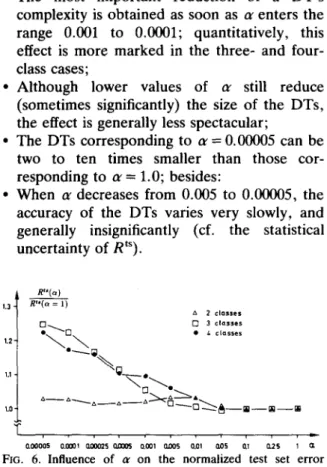
• The most important reduction of a DT's complexity is obtained as soon as a~ enters the range 0.001 to 0.0001; quantitatively, this effect is more marked in the three- and four- class cases;
• Although lower values of tr still reduce (sometimes significantly) the size of the DTs, the effect is generally less spectacular;
• The DTs corresponding to tr = 0.00005 can be two to ten times smaller than those cor- responding to te = 1.0; besides:
• When cr decreases from 0.005 to 0.00005, the accuracy of the DTs varies very slowly, and generally insignificantly (cf. the statistical uncertainty of RtS). R"(¢,) R " ( a = 1) z~ 2 classes [ - ] ~ . I'~ 3 classes • \ ~ \ • , o , . . . 1.3 1.2 1.1- 1.0 T
FIG. 6. Influence of a~ on t h e n o r m a l i z e d test set e r r o r estimate. N = 500, M = 1500.
Figures 5 and 6 illustrate graphically the above observations in the two-, three-, and four-class situations. In each class, the curves represent the mean relative variations of the size, (Nt), and of the misclassification r a t e ( R t S ) , of 132 DTs (each point of the curves represents the mean value of 12 different DTs built for the corresponding value of or).
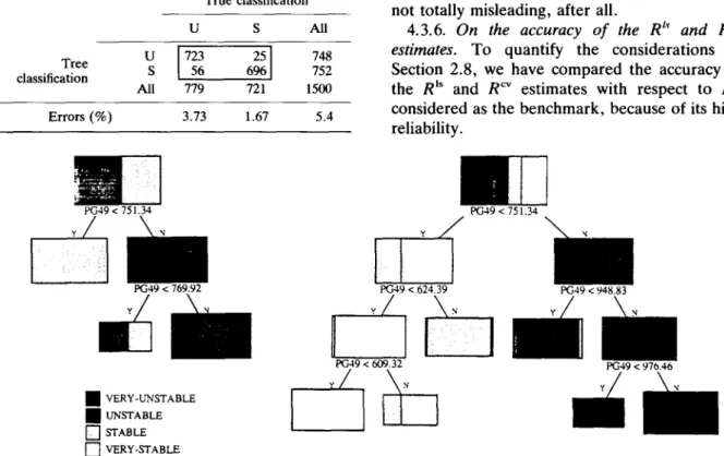
The following example provides an insight into the way the value of tr operates in the particular case where the attributes contain less informa- tion (i.e. the "less separable" case). This corresponds to a LS of 500 states, a biclass pattern, and seven values of tr ranging from 1.0 (the nodes are split until they are all leaves) to 0.00005 (extremely "cautious" behavior). Seven DTs were accordingly built, for the contingency #2, where the most important attribute (PG122, the active power generated at the bus #112) was removed from the list of candidate attributes. Table 3 summarizes the results. Columns 2-5 list the number of respectively test nodes, leaves, deadends, total. (Note that since the DTs are binary, they always have as many nodes as the double of test nodes plus one: Nt = 2Nts + 1). The following three columns of Table 3 provide the misclassification rate as appraised by respectively the resubstitution, the test sample, and the cross-validation estimate; incidentally, observe the optimistic character of R ~S, and to a much lesser extent, of Rcv.
One can see that decreasing the value of c~ in the interval [ 1 . 0 . . . 0.01] not only drastically reduces the complexity of the DTs but it moreover significantly improves their accuracy.
On the other hand, in the interval
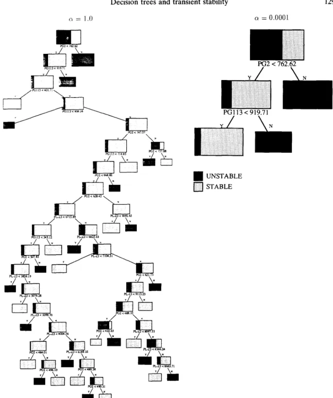
[ 0 . 0 1 . . . 0.00005] the size of the DTs decreases moderately, whereas their accuracy remains unchanged. Figure 7 is an eloquent illustration of the decrease in complexity: for o~=1, N, amounts to 63, whereas for o~=0.0001 Nt reduces to 5. Notice that the two DTs have the same structure nearby their respective roots.
The general conclusions are the following: 1. The statistical hypothesis test is able to detect and identify the deadends in a very efficient and
TABLE 3. IMPACT OF ~ ON COMPLEXITY AND ACCURACY IN THE LESS SEPARABLE CASE OF A BICLASS PATTERN N = 500,
M = 1500, CONTINGENCY # 2 o~ Nt~ N~ Naa N t R'~(%) R t ~ ( % ) R ¢ ~ ( % ) 1.00000 31 32 0 63 0.6 11.9 10.2 0.10000 27 26 2 55 1.0 11.5 7.4 0.01000 3 3 1 7 6.0 8.8 7.4 0.00500 3 3 1 7 6.0 8.8 7.4 0.00050 3 3 1 7 6.0 8.8 7.4 0.00010 2 2 1 5 6.0 8.8 7.2 0.00005 2 2 1 5 6.0 8.8 7.2
reliable manner, provided that the value of tr is lower than 0.001;
2. Using tr values below 0.001 provides the twofold benefit of reduced complexity and improved reliability; this effect is even more important in the less separable cases, where the "variance" effect can be very important;
3. The precise value of tr, realizing the best compromise between what are called "variance" and "bias" in Section 2, lies somewhere in between 0.001 and 0.00005; the lower the number of classes, the lower the "optimal" value; moreover, the higher the contribution of the variance effect (e.g. the lesser the informa- tion contained in the candidate attributes), the lower the optimal value of re;
4. Anyhow, the bias effect remains very low (it would probably appear markedly for values of tr much lower than 0.00005); thus the precise value of tr is practically of no concern, as long as it lies in the range [0.001... 0.00005];
5. Hence, considering that for a required accuracy, the smaller the trees the better, it is advisable to use or=0.0001 in all cases; sometimes it is even preferable to sacrifice a little accuracy for simplicity of the tree structure.
Remark. Although the above conclusions are drawn in the specific context of transient stability, preliminary investigations indicate that they correspond to the very nature of the statistical hypothesis test, and should remain valid in general. (Wehenkel, 1990).
4.3.3. On the size of the LS. One may distinguish the following three questions:
How does the size of the LS influence a DT's complexity and accuracy?
What is the minimal number of learning states required to achieve an acceptable accuracy?
How "stable" is the DT when the LS changes? or stated otherwise, how sensitive is the structure of the DT to the changes of the LS?
Qualitatively, according to the principle of the inductive inference method, one can say that, for a given value of c~, increasing the size of the LS will generally (although not necessarily) increase the complexity and the accuracy.
Quantitatively, the answer to the first two questions strongly depends on the particular application of concern and especially on the intricacy of the underlying relationship between the attributes and the classification pattern. The more intricate this relation, the larger the sufficiently accurate DTs and the larger the LS required to build them in a reliable fashion.
As regards stability, we generally found that the nodes near the root of the DT (which
o -- 1.0 = 0.0001 PG2 < 162.~ 1~113. 91971 PG2 < 7,17.07 P~II3 < 714 ~5 PG2<~ p L+/.3 O71589 90~ PG 113 < 5,~.3.12 I'v32 < 507 83 ~ r P["+7+3 < ~ p ~ 9 . 1 i P L - Z 3 < 5O76.28 pt.-Z3 < 5O99.7O . " • .
m
1~32 < 757.88 ~ 3 ~ . 7 1li
FIG. 7. Typical variation of tree structure with ol
express the most relevant relationships) do not change much when N increases, w h e r e a s the lower nodes (expressing the details) can change m o r e significantly.
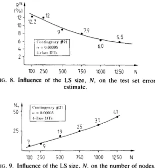
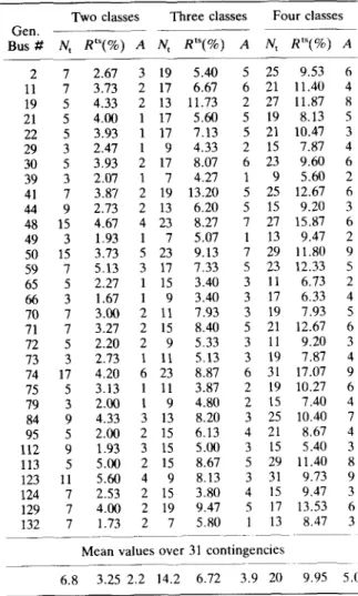
To illustrate and support these considerations, we conducted the following investigations: for the contingency # 2 1 , r e = 0 . 0 0 0 0 5 , and in the four-class p a t t e r n , six D T s were built with N, the size of the learning set, varying f r o m 100 to 1250 states. Each D T was tested on the basis of the remaining M - - 2 0 0 0 - N test states. T h e results
PG2 < 762.62 PG113 < 919.71
k l
m
~ UNSTABLE [ ] S T A B L E(biclass DTs for contingency #2, N = 500).
are r e p r e s e n t e d graphically in Figs. 8 and 9. O n e can see that for increasing values of N the e r r o r rate decreases f r o m 12.2% to 5 . 5 % , w h e r e a s the n u m b e r of the trees' nodes increases f r o m 9 to 43. A t the same time, the n u m b e r of retained attributes is found to increase f r o m 2 to 11. Figure 10 provides two D T s , built for N - - 2 5 0 and 750, and having respectively N t - - 9 and 25, and A = 2 and 7. O b s e r v e the stability of the DTs.
These and m a n y o t h e r similar results indicate