QoS in IoT networks based on link quality prediction

(1)

HAL Id: hal-03162826

https://hal.archives-ouvertes.fr/hal-03162826

Submitted on 8 Mar 2021

HAL is a multi-disciplinary open access

archive for the deposit and dissemination of

sci-entific research documents, whether they are

pub-lished or not. The documents may come from

teaching and research institutions in France or

abroad, or from public or private research centers.

L’archive ouverte pluridisciplinaire HAL, est

destinée au dépôt et à la diffusion de documents

scientifiques de niveau recherche, publiés ou non,

émanant des établissements d’enseignement et de

recherche français ou étrangers, des laboratoires

publics ou privés.

QoS in IoT networks based on link quality prediction

Chérifa Boucetta, Boubakr Nour, Albéric Cusin, Hassine Moungla

To cite this version:

Chérifa Boucetta, Boubakr Nour, Albéric Cusin, Hassine Moungla. QoS in IoT networks based on

link quality prediction. IEEE International Conference on Communications (ICC), 2021, Montreal

(virtual), Canada. pp.1-7. �hal-03162826�

(2)

QoS in IoT Networks based on Link Quality

Prediction

Chérifa Boucetta

∗

, Boubakr Nour

‡

, Albéric Cusin

§

, and Hassine Moungla

§ ¶

∗_{Université de Reims Champagne-Ardenne, CReSTIC EA 3804, 51097, REIMS, FRANCE}

§_{School of Computer Science, Beijing Institute of Technology, Beijing, China}

‡_{Université de Paris, LIPADE, F-75006 Paris, France}

¶_{UMR 5157 CNRS, Telecom SudParis, Institut Polytechnique de Paris, Palaiseau 91120, France}

Email: [email protected], [email protected], [email protected], [email protected]

Abstract—The success of the Internet of Things (IoT) depends on the ability to provide reliable communication to the billions of devices that are used in many applications. In essence, estimating the quality of wireless links ensures the optimization of several protocols, reduces the end-to-end latency, and increases the reliability and the network lifetime. In this paper, we study the link quality in the Time Slotted Channel Hopping (TSCH) network by analyzing the received signal strength (RSSI) and error rates. The objective is to understand the temporal properties of these parameters which is important to select the appropriate channels for the critical applications and to enhance the Quality of Service (QoS) of the network. We apply machine learning techniques to a real dataset collected from a testbed IoT network deployed at Grenoble, France. We define five classes and present a classification of the 16 channels by comparing the performances of KNN (k-Nearest Neighbor) and LSTM (Long Short-Term Memory) algorithms.

Index Terms—Internet of Things (IoT), Link quality, QoS, TSCH

I. INTRODUCTION

With the deployment of high speed networks and the rapid growth of smart devices, the Internet of Things (IoT) has gained wide acceptance and popularity. The number of Iot devices is estimated at 50 billion in 2020 [1]. They are used in several fields of application such as: industry, energy saving, home automation, security, smart cities, etc. These applications have a great impact on the quality of life of people and also lead to economic benefits. The IoT objects are low-cost and easy to deploy. Many architectures, operating systems and protocols are defined for the IoT networks [2], [3]. Conse-quently, different challenges may arise during the deployment of IoT applications including the scalability, the diversity of applications requirements, channel utilization, device’s re-source limitation such as energy efficiency, processing capacity and memory size [4]–[6]. Furthermore, radio signals are very sensitive to noise, interference and multi-path distortions [7]. Hence, the Quality of Service (QoS) depends on the quality estimation of the communication links between nodes which have an impact on the routing and data gathering [8].

Quality approaches have been proposed at various layers of the IoT architecture and take into consideration a number of different QoS factors [9]. For example, the routing protocols of these networks use various link quality estimators to spec-ify the best available paths considering higher-quality links.

Furthermore, machine learning algorithms can be employed to build link quality predictors. These algorithms assume an initial model that can be used to generate predictions in real time without any computational capabilities. The machine learning model can be thereafter updated every time a new quality value is observed in the link with the aim of improving the accuracy of the initial model and also adapting it to the changes observed in the link. Several approaches for the link quality estimation are proposed in literature. In this paper, we focus on data link layer by studying the quality of wireless links. The objective is to anticipate the link breakage and assign links with good quality to critical applications which improves the Quality of Experience (QoE) provided by the network. Generally, the quality of a link is estimated as a proportion of successfully received packets. Hence, the goodness of a link is linear to the proportion of received packets. For this reasons, we study the link quality metrics and then we apply Machine Learning (ML) algorithms to classify and predict the quality of wireless links. This quality is usually measured as a single value, such as Received Signal Strength Indicator (RSSI), Link Quality Indicator (LQI) or the packet delivery ratio (PDR) [10]. We apply KNN and LSTM machine learning schemes and we consider a real data-set extracted from the Grenoble testbed of the FIT IoT-lab. .

The rest of the paper is structured as follows; in Section II we present a brief review of link quality metrics and we focus on machine learning techniques used in link quality prediction. In section III, we describe the test bed dataset, the prediction procedure and then, we present comprehensive analysis of ML approaches applied on different metrics. Finally, section IV concludes the paper.

II. BACKGROUND& RELATEDWORK

In the following, we briefly describe the most used link quality metrics in the literature, and then we review two of the important machine learning algorithms that can be applied in the predictions in IoT networks.

A. Link Quality in IoT

A link characterizes a path allowing the exchange of data between a sender and a receiver. Evaluating the quality of links is crucial because it provides valuable information on

(3)

the quality of transmission and avoid collisions. In essence, wireless links with a bad quality would generate many re-transmissions of the same packets which increases delivery latency and decreases network lifetime by wasting node en-ergy. However, a stable link guarantees a successful packet reception.

Two types of metrics are defined to estimate the link quality in IoT: hardware-based metrics and software-based metrics.

Hardware-based metrics. They are defined to estimate the the Received Signal Strength (RSSI) and the Link Quality Indication (LQI) of the received packet [11]. They include:

• Received Signal Strength Indicator (RSSI) is an

estima-tion of the received signal power in the channel. It is measured over the first 8 symbols following the start delimiter of a frame. When there is no transmission, the register gives a background noise.

• Link Quality Indication(LQI) indicates the quality of the

received signal computed using the signal to noise ratio. The routing metric at the network layer depends on this measure.

• Signal to Noise Ratio(SNR) denotes the strength of the

signal. It is the difference between the received signal strength and the background noise.

To estimate SNR, the receiver records at first the RSSI of the received packet, then it has to measure the background noise. RSSI of a signal is defined as:

RSSI[dBm] =10 log10(𝑃𝑅 𝑃+ BKG_noise[dBm]) (1)

where 𝑃𝑅 𝑃 and 𝐵𝐾𝐺𝑛𝑜𝑖 𝑠𝑒 are the power of the received

packet and the background noise respectively.

Because the RSSI of the ambient noise is estimated as

10𝑙𝑜𝑔10(𝐵𝐾𝐺𝑛𝑜𝑖 𝑠 𝑒), the equation of the SNR is the following:

SNR[dBm] = RSSI[dBm] − BKGnoise[dBm] (2)

The RSSI and the LQI metrics are correlated with the good-ness of a signal and are computed over each received packet. Numerous existing researches explored the link behavior in literature. The authors in [12] presented an experimental study of wireless link quality variation over a period of several days in a sensor network placed in two different indoor office environments. Kola et al. [13] analyzed the received signal strength and error rates in an IEEE 802.11 indoor wireless mesh network.They demonstrated that statistical distribution and memory properties vary across different links, but are predictable.

Software-based metrics. The software-based estimators are further split into into three categories [14]:

• (Packet-Delivery Ratio)(PDR) is defined as the ratio of

the successful received packets to the total number of send packets.

• Requested Number of Packets(RNP) It counts the average

number of packet transmissions/re-transmissions required before a successful reception.

• Score-based is used to provide a score or a label

iden-tifying the link quality without referring to a physical phenomena.

These software-based metrics can be gathered either on the receiver, transmitter or both sides. Several works studied the link quality based on hardware and software metrics. In [15], the authors evaluated the relative accuracy of four metrics for capturing the quality of a wireless link: RSSI, SINR, PDR and BER (Bit-Error Rate) by conducting experiments with multiple transmission rates and varying levels of interference on a large set of links. A two stage classification was proposed in [16], in which a very large fraction of links are immediately either deemed usable or not, while the remaining ones need a bit more testing before they are advertised by the routing protocol as good or weak links. The Authors in [17] proposed a prediction based cooperative scheme through which the prob-lem of "when to relay" and "who to relay" are decided in an optimal way. Also, the authors of [18] showed cooperative two relay communication with opportunistic relaying significantly mitigates interference of the whole network. However, more recent works conducted in [19] studied an effective scheme for joint two-hop cooperative communication integrated with transmit power control for interference mitigation.

Generally, the existing metrics ensure either stability or accuracy, depending on their types, but rarely both. Overall, previous studies tried to classify links and discussed link asymmetry. They claimed that intermediate links are highly unstable. In this context, we further predict the link quality using hardware and software based metrics. We mainly fo-cus on link classifications according to PDR as well as on the temporal and spatial fluctuation of RSSI and LQI. The prediction of the values of the link metrics at a given time will allow the adaptation of the data transmission. Indeed, in wireless networks, collisions between data packets can occur. If we know that a link at a given time has a high chance of having collisions, then we can shift the transmission to a more favorable time and therefore less prone to collisions. To make these prediction, we use machine learning algorithms. B. Machine Learning Techniques

Due to the ability to process and learn from large amount of data traces, the use of ML techniques in link quality estima-tions is promising to significantly improve the performance of the networks. Data sets can be collected across various technologies, topologies and mobility scenarios. Several con-tributions can be found in the literature exploiting ML such as classification, regression and clustering techniques in link quality predictions. In this paper, we used KNN (K-Nearest Neighbour) and LSTM (Long Short-Term Memory) to predict the short term evolution of link quality, in order to switch the data transmission on a better quality link. K-Nearest Neighbour. KNN is a supervised learning model that could predict the link quality state based on a small correlative part of data [20]. In essence, it has no training phase. The training data is used when making predictions to classify the data.

(4)

KNN It searches the K most similar feature vectors within the historical database to predict future values. It defines a simple structure with high computation efficiency. In general, the prediction performance is influenced by the attributes of datasets. For that, KNN has the ability to find out the most similar historical patterns and ignore other dissimilar patterns of the dataset.

KNN has been applied to address a variety of problems within the context of wireless networks other than link quality prediction. KNN has been used for for traffic state prediction [21], anomaly detection, energy consumption, etc.

Long Short-Term Memory. LSTM is a is a deep learning approach making predictions using historical data as a training set. It learns over long sequences (keep or forget informa-tion) [22]. This feature differentiates it from regular multi-layer neural networks that do not have memory and can only learn a mapping between input and output patterns.

The LSTM network is composed of three layers: : Input, Hidden, and Output Layer [23]. It is constituted of memory blocks with self-loops. Each memory block is composed of special multiplicative units called gates. The memory blocks learn over arbitrary vector representation of the input time-series. The data is filtered with a set of weights and the help of three gates. The input and forget gate, both work on the state of memory blocks. The role of the input gate is to decide what incoming data will be stored in memory, while forget-gate is aimed at selectively forgetting information that is no longer required for the LSTM understanding. It defines how long data will be stored. Finally, the output gate is responsible for picking useful information and dispensing it out as an output. The LSTM learns to keep only pertinent information to make predictions. This is achieved during the retro-propagation (training phase).

III. WIRELESS LINK QUALITY PREDICTION

A. Dataset

In this study, we have used a dataset provided by IoT-LAB1

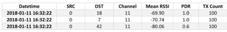
at Grenoble, France. We were able to access to 50 IoT nodes (sensor and actuator) connected on 16 channels during 48 hours, with an overall of 6000 data exchanges per channel. For each record, we collected the daytime, source, destination, channel, average RSSI, PDR, and the number of packets sent. Table I shows a raw dataset sample.

TABLE I: Raw dataset sample.

Datetime SRC DST Channel Mean RSSI PDR TX Count 2018-01-11 16:32:22 0 18 11 -69.90 1.0 100

2018-01-11 16:32:22 0 7 11 -70.74 1.0 100

2018-01-11 16:32:22 0 42 11 -80.06 0.6 100

SRC DST Channel Mean RSSI PDR Link Classes PDR Difference RSSI Difference

1 0 7 11 -70.74 1.0 0 0.0 -0.84

2 0 42 11 -80.6 0.6 2 -0.4 -9.32

3 0 28 11 -68.46 1.0 0 0.4 11.60

Excellent Good Average Bad Very Bad

PDR ≥ 0.9 AND RSSI ≥ -80 PDR ≥ 0.9AND -80 < RSSI < -90 OR 0.9 < PDR < 0.1 AND RSSI ≥ -80 0.9 < PDR < 0.1 AND -80 < RSSI < -90 PDR ≤ 0.1 AND -80 < RSSI < -90 OR 0.9 < PDR < 0.1 AND RSSI ≤ -90 PDR ≤ 0.1 AND RSSI ≤ -90

Datetime SRC DST Channel Mean RSSI PDR TX Count

We are, therefore, in the case of time series. So the daytime of sending becomes the index of our matrix. We have then 6 variables. After a quick glance at the means, standard deviations, and variances of the different variables, we can eliminate the last variable (the number of packets sent) because

1_{IoT-LAB: www.iot-lab.info}

it does not vary. After cleaning the dataset, we need to perform feature engineering. Hence, we added the difference from one transmission to another for the average RSSI as well as for the PDR. These features are calculated based on the following formulas:

RSSI𝑡( 𝐴, 𝐵) =

Í

𝑖 rssi𝑖( 𝐴 → 𝐵)

Í Packet( 𝐴 → 𝐵) (3)

where 𝐴 is the sender and 𝐵 is the receiver, rssi𝑖 represents

the RSSI of the 𝑖𝑡 ℎ

packet sent by A and received by B.

PDR𝑡( 𝐴, 𝐵) =

Í ACK(𝐵 → 𝐴)

Í Packet( 𝐴 → 𝐵) (4)

In this case, a packet sent by node A is counted as received by B if and only if B sends an acknowledgment. The PDR ranges from 100% if the node received all packets, to 0% if it received zero packet.

Additionally, we also want to rank links based on their quality. So we defined the five classes, as shown in Table II.

TABLE II: Classes of link quality.

Since the different variables’ values do not have the same range, we need to scale the values before passing them to the model. Here, the RSSI varies between -95 and -25 while the PDR varies between 0 and 1. Therefore, we have to sort all the variables in the same order of magnitude so that the model does not give more importance to one variable than another. Table III shows a sample of dataset after the cleaning process.

TABLE III: Cleaned dataset sample.

Datetime SRC DST Channel Mean RSSI PDR TX Count 2018-01-11 16:32:22 0 18 11 -69.90 1.0 100

2018-01-11 16:32:22 0 7 11 -70.74 1.0 100

2018-01-11 16:32:22 0 42 11 -80.06 0.6 100

SRC DST Channel Mean RSSI PDR Link Classes PDR Difference RSSI Difference

1 0 7 11 -70.74 1.0 0 0.0 -0.84

2 0 42 11 -80.6 0.6 2 -0.4 -9.32

3 0 28 11 -68.46 1.0 0 0.4 11.60

Datetime SRC DST Channel Mean RSSI PDR TX Count

B. Models

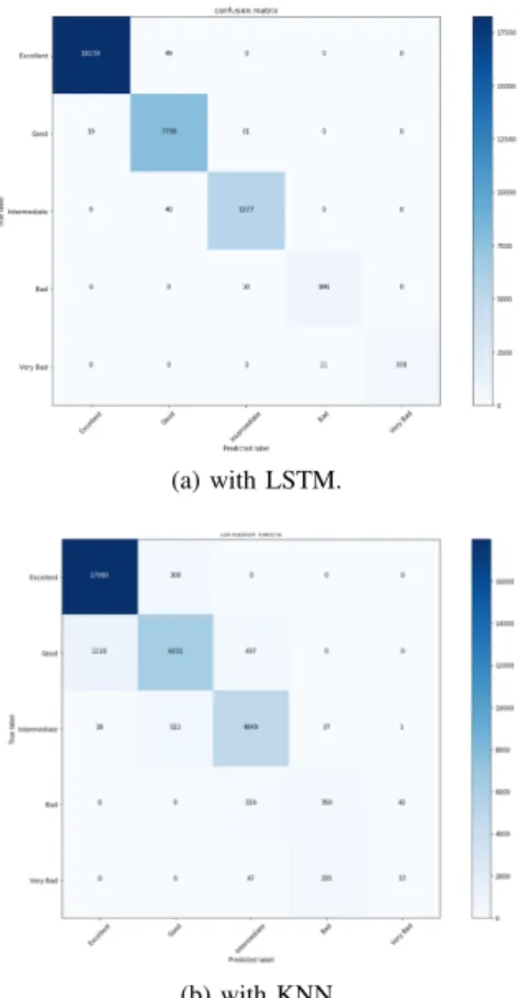
Starting with LSTM and KNN, the model has to predict one of the 5 link quality categories above. Startin with LSTM, Fig. 1a indicates for each real class, which class the model predicted. We also notice the disparity in the classes of links. More than half of the links are “Excellent” and only a tiny fraction are “Very Bad”.

This step allowed us to know that the choice of LSTM cells was the right choice given the better results compared to the results with KNN (Figure 1b). However, to reach the target goal, we need to predict RSSI and PDR metrics to identify the quality of a link. Here, we have created a new model with regression problem. After some testing, we found that the predictions of RSSI and PDR did not react exactly the same way and therefore the model had to be adapted to the metric.

(5)

(a) with LSTM.

(b) with KNN

Fig. 1: Confusion matrix for the classification of links.

C. Learning and Predictions

Before tackling the model parameters, we tested 3 different scalings: “Robust Scaler”, “Standard Scaler”, and “MinMax Scaler”. We have then developed a simple model where we can observe the different performances.

As shown in Fig. 2, the scaling gave different results for RSSI and PDR metrics. Here, we decide to chose the scaler with the lowest loss, which means that we selected “MinMax Scaler” for the RSSI, and “Standard Scaler” for the PDR. We also split the data to 70% for training, and 30% for test. D. Optimizers, Loss Function, and Number of Epochs

Now, we need to predict the RSSI and the PDR so that we could rank the links according to their quality. To decide on the number of epochs, we had to determine it based on the curves and see when the loss was no longer changing. By doing regression work, the chosen loss function was the root mean square error. The results were slightly different, if not worse with other functions. Looking at the scaling curves, 1000 epochs seemed suitable. Then we tested different optimizers for the two models. Fig. 3 shows the accuracy of the model according to the epochs and the chosen optimizer. From the obtained results, we were able to disqualify Adagrad for RSSI and SGD for PDR since they are too slow to learn or even unable at a time. However, the results for Nadam and Adam have been similar for both metrics.

0 200 400 600 800 1000 Number of epochs 0.0 0.2 0.4 0.6 0.8 1.0 Lo ss Va lue Robust Standard MinMax (a) RSSI. 0 200 400 600 800 1000 Number of epochs 0.00 0.02 0.04 0.06 0.08 0.10 0.12 0.14 Lo ss Va lue Robust Standard MinMax (b) PDR

Fig. 2: Model precision according to the number of epochs according to the chosen scaling.

(a) RSSI.

(b) PDR

Fig. 3: Accuracy of the model according to the epochs and the chosen optimizer.

E. Number of Layers and Neurons

The more layers and neurons the model has, the greater number of calculations and therefore the longer the execution

(6)

(a) RSSI.

(b) PDR

Fig. 4: Channel 11 metric predictions (sample prediction, parameters: Adam, MAE, 4505 training data, 4 hidden layers of 128, 64, 32 and 16 neurons).

time. We started with a 4 hidden layer model of 128, 64, 32, and 16 neurons (LSTM cells), the obtained results are shown in Fig. 4. The execution times were relatively fast but the performance poor. Given the rather mediocre results observed, we made two hypotheses: (a) there is not enough training data for the model to correctly capture the complexity of channel quality variations, and (b) the chosen model is not efficient enough to predict values. Therefore, we decided to increase in a semi-synthetic way, by creating new data from what we already have, and hence allow better learning.

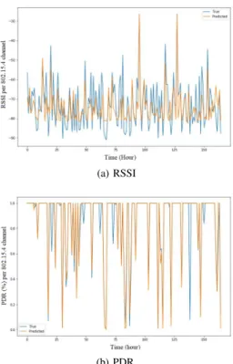
After the first test, and by increasing only the number of data, the results are immediately better. Although the predictions for RSSI are slightly improved (Fig. 5a), the performance of PDR prediction is greatly improved (Fig. 5b). Besides, by modifying the number of neurons to 256 for the 4 layers of the model, the performance becomes excellent for the predictions of RSSI and PDR (Fig. 6). The calculation time is approximately one hour.

F. Prediction Accuracy:

In this work, we have two almost identical models, only the activation function of the output layer is different, near for the RSSI and sigmoid for the PDR. The input data differs in its scaling, the "MinMax scaler" is used for RSSI data, and the "Standard scaler" is used for PDR data.

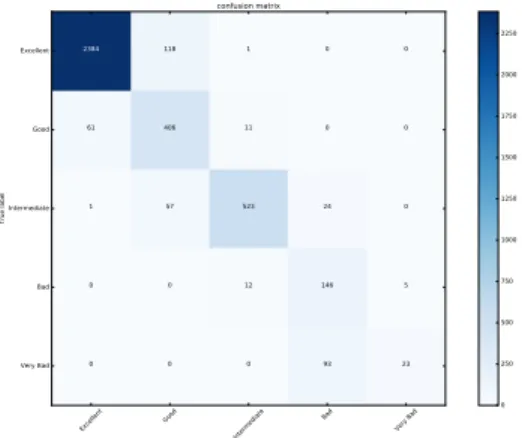
By predicting the RSSI and PDR metrics, we were able to predict the quality of a link according to different classes (Table II), which gives us a confusion matrix as shown in Fig. 7. We can normalize this matrix in order to obtain percentages

(a) RSSI

(b) PDR.

Fig. 5: Metric predictions for channel 11 with increased data volume (sample prediction, parameters: Adam, MSE, 9018 training data, 4 hidden layers of 128, 64, 32 and 16 neurons).

(a) RSSI.

(b) PDR.

Fig. 6: Metric predictions for channel 11 with increased data volume (sample prediction, parameters: Adam, MSE, 4 hidden layers of 256 neurons).

(7)

Excelle nt _Good Interme diate Bad Very Ba d Predicted label Excellent Good Intermediate Bad Very Bad Tru e l ab el 2384 118 1 0 0 61 406 11 0 0 1 57 523 24 0 0 0 12 146 5 0 0 0 93 23 confusion matrix 0 250 500 750 1000 1250 1500 1750 2000 2250

Fig. 7: Confusion matrix of the classes.

Excelle nt _Good Interme diate Bad Very Ba d Predicted label Excellent Good Intermediate Bad Very Bad Tru e l ab el 0.95245705153815420.047143427886536160.00039952057530962844 0.0 0.0 0.127615062761506280.84937238493723850.02301255230125523 0.0 0.0 0.001652892561983471 0.094214876033057850.86446280991735540.03966942148760331 0.0 0.0 0.0 0.07361963190184050.89570552147239270.03067484662576687 0.0 0.0 0.0 0.80172413793103450.19827586206896552 confusion matrix 0.0 0.1 0.2 0.3 0.4 0.5 0.6 0.7 0.8 0.9

Fig. 8: Normalized confusion matrix.

depicted in Fig. 8.

On the diagonal, we can find good predictions, and on the rest of the lines, we find bad predictions. We can easily see that the “Excellent” quality is predicted very well. Conversely, "Very Bad" quality is very poorly predicted. This is explained by the training data, which is uneven and which includes much more "Excellent" quality and very little "Very Bad" quality. One solution to this problem would be to homogenize the data to have as much quality of each class.

IV. CONCLUSION

In this paper, we proposed to predict link quality in IoT networks. We studied two link quality estimators: a hardware one, RSSI, and a software one, PDR. We compared the accuracy provided by different machine learning techniques: KNN and LSTM. Considering bad links in routing protocols penalizes the network performances in terms of end-to-end latency, end-to-end reliability and network lifetime. In essence, we demonstrate the importance of the prediction techniques in the case of critical application and to improve the QoS of the network. The next phase of the project will therefore be to use these models and to be able to predict for a real network, the quality of the links in order to optimize communications. It will be necessary to test, if this method can be used for a larger number of nodes and therefore of data. Nevertheless,

if this method is viable, it could be used in various fields of application such as security, with the case of critical applications which require reliable and fast communication, or even for smart cities comprising networks of sensors of size.

REFERENCES

[1] A. Al-Fuqaha et al., “Internet of things: A survey on enabling tech-nologies, protocols, and applications,” IEEE Communications Surveys & Tutorials, vol. 17, no. 4, pp. 2347–2376, 2015.

[2] M. Chernyshev et al., “Internet of Things (IoT): Research, Simulators, and Testbeds,” IEEE Internet of Things Journal, 2017.

[3] B. Nour et al., “ICN publisher-subscriber models: Challenges and group-based communication,” IEEE Network, vol. 33, no. 6, pp. 156–163, 2019.

[4] M. J. Ali et al., “Interference avoidance algorithm (iaa) for multi-hop wireless body area network communication,” in International Confer-ence on E-health Networking, Application & Services (HealthCom). IEEE, 2015, pp. 540–545.

[5] M. Ali et al., “Distributed scheme for interference mitigation of WBANs using predictable channel hopping,” in IEEE international conference on

e-Health networking, applications and services. IEEE, 2016, pp. 1–6.

[6] H. Moungla et al., “Distributed interference management in medical wireless sensor networks,” in IEEE annual consumer communications

& networking conference (CCNC). IEEE, 2016, pp. 151–155.

[7] C. Boucetta et al., “An IoT Scheduling and Interference Mitigation Scheme in TSCH using Latin Rectangles,” in IEEE Global

Commu-nications Conference (GLOBECOM). IEEE, 2019, pp. 1–6.

[8] R. Imran et al., “Quality of experience for spatial cognitive systems within multiple antenna scenarios,” IEEE transactions on wireless com-munications, vol. 12, no. 8, pp. 4153–4161, 2013.

[9] A. Churcher et al., “An Experimental Analysis of Attack Classification Using Machine Learning in IoT Networks,” Sensor, 2021.

[10] N. Baccour et al., “Radio link quality estimation in wireless sensor networks: A survey,” ACM Transactions on Sensor Networks (TOSN), vol. 8, 09 2012.

[11] M. L. F. Sindjoung et al., “Wireless Link Quality Prediction in IoT Networks,” in International Conference on Performance Evaluation and Modeling in Wired and Wireless Networks (PEMWN). IEEE, 2019, pp. 1–6.

[12] D. LaI et al., “Measurement and Characterization of Link Quality Metrics in Energy Constrained Wireless Sensor Networks,” vol. 1, 01 2004, pp. 446 – 452 Vol.1.

[13] V. Kolar et al., “Measurement and Analysis of Link Quality in Wireless Networks: An Application Perspective,” INFOCOM IEEE Conference on Computer Communications Workshops, pp. 1–6, 2010.

[14] M. Kirubasri et al., “A Study on Hardware and Software Link Qual-ity Metrics for Wireless Multimedia Sensor Networks,” International Journal of Advanced Networking and Applications, 2016.

[15] A. Vlavianos et al., “Assessing link quality in IEEE 802.11 Wireless Networks: Which is the right metric?” 10 2008, pp. 1 – 6.

[16] H.-J. Audeoud et al., “Quick and Efficient Link Quality Estimation in Wireless Sensors Networks,” 02 2018, pp. 87–90.

[17] H. Feng et al., “Prediction-based dynamic relay transmission scheme for Wireless Body Area Networks,” in IEEE International Symposium on Personal Indoor and Mobile Radio Communications (PIMRC), 2013. [18] J. Dong et al., “Opportunistic relaying in wireless body area networks:

Coexistence performance,” in IEEE International Conference on

Com-munications (ICC). IEEE, 2013, pp. 5613–5618.

[19] J. Dong et al., “Joint relay selection and transmit power control for wireless body area networks coexistence,” in IEEE International

Conference on Communications (ICC). IEEE, 2014, pp. 5676–5681.

[20] H. Yu et al., “A Special Event-Based K-Nearest Neighbor Model for Short-Term Traffic State Prediction,” IEEE Access, vol. 7, pp. 81 717– 81 729, 06 2019.

[21] L. Kuang et al., “Predicting duration of traffic accidents based on cost-sensitive Bayesian network and weighted K-nearest neighbor,” Journal of Intelligent Transportation Systems, vol. 23, no. 2, pp. 161–174, 2019. [22] X. Shi et al., “Convolutional LSTM Network: A Machine Learning

Approach for Precipitation Nowcasting,” 06 2015.

[23] Z. Zhao et al., “LSTM network: a deep learning approach for short-term traffic forecast,” IET Intelligent Transport Systems, 2017.