HAL Id: hal-01228488
https://hal.inria.fr/hal-01228488
Submitted on 19 Nov 2015
HAL is a multi-disciplinary open access archive for the deposit and dissemination of sci-entific research documents, whether they are pub-lished or not. The documents may come from
L’archive ouverte pluridisciplinaire HAL, est destinée au dépôt et à la diffusion de documents scientifiques de niveau recherche, publiés ou non, émanant des établissements d’enseignement et de
Jacques Nicolas, Pierre Peterlongo, Sébastien Tempel
To cite this version:
Jacques Nicolas, Pierre Peterlongo, Sébastien Tempel. Finding and Characterizing Repeats in Plant Genomes. David Edwards. Plant Bioinformatics: Methods and Protocols, Humana Press -Springer Science+Business Media, pp.365, 2015, Methods in Molecular Biology, 978-1-4939-3166-8. �10.1007/978-1-4939-3167-5_17�. �hal-01228488�
Finding and characterizing repeats in plant genomes
Jacques Nicolas1 1 , Pierre Peterlongo1 and Sébastien Tempel2
1 Irisa/Inria Centre de Rennes Bretagne Atlantique,
Campus de Beaulieu, 35510 Rennes cedex, France
2LCB, CNRS UMR 7283
31 Chemin Joseph Aiguier - 13402 Marseille cedex 20, France
Abstract: Plant genomes contain a particularly high proportion of repeated structures of
various types. This chapter proposes a guided tour of available software that can help biologists to look for these repeats and check some hypothetical models intended to characterize their structures. Since transposable elements are a major source of repeats in plants, many methods have been used or developed for this large class of sequences. They are representative of the range of tools available for other classes of repeats and we have provided a whole section on this topic as well as a selection of the main existing software. In order to better understand how they work and how repeats may be efficiently found in genomes, it is necessary to look at the technical issues involved in
the large--scale search of these structures. Indeed, it may be hard to keep up with the profusion of proposals in this dynamic field and the rest of the chapter is devoted to the foundations of the search for repeats and more complex patterns. The second section introduces the key concepts that are useful for understanding the current state of the art in playing with words, applied to genomic sequences. This can be seen as the first stage of a very general approach called linguistic analysis that is interested in the analysis of natural or artificial texts. Words, the lexical level, correspond to simple repeated entities in texts or strings. In fact, biologists need to represent more complex entities where a repeat family is built on more abstract structures, including direct or inverted small repeats, motifs, composition constraints as well as ordering and distance constraints between these elementary blocks. In terms of linguistics, this corresponds to the syntactic level of a language. The last section introduces concepts and practical tools that can be used to reach this syntactic level in biological sequence analysis.
Keywords: Repeats, Transposon, Indexing, Algorithmics on words, Pattern matching.
1. Introduction
A salient feature of eukaryotic genomes is the number of repeated sequences that they contain. Many processes contribute to this accumulation of genomic material. Even if the polyploidy speciation mechanism were not taken into account, plant genomes are particularly rich in copy events that explain the remarkable range of their size variation and may considerably increase this size. Indeed, the genome length world record,
1.5x10¹¹ DNA base pairs, is currently held by a plant, Paris japonica, an octoploid native
to sub-alpine regions of Japan. The aim of this chapter is to propose several methods that help identify the various repeats that populate DNA sequences. The objective is more to collect and explain key concepts rather than to present an exhaustive and somewhat tedious study of the search for the various known repeat types, which may quickly have become obsolete.
In fact, due to its importance, we will describe in detail only the exploration of the major source of repeats, the transposable element (TE) super-class. Transposable elements often account for up to 40% of plant genomes and, for example, account for about 60% of Solanum lycopersicum and Sorgum bicolor, and 80% of the Triticum aestivum or the Zea mays genome sizes. A whole section is devoted to practical methods that have been developed to extract TEs. This includes both generic tools and tools tailored for a particular class of RNA or DNA transposons. Another important class of repeats in some plants, such as Olea europaea (1), the tandem (or satellite) repeats, are not treated specifically, although some pointers to ab initio methods for transposable elements, such as RepeatExplorer (2), may be useful for the search of tandem repeats on reduced sets of genomic reads. We refer the interested reader to a fine review on this topic in (3).
We then propose a more advanced section on the algorithmic basis of the detection of copies. This will help the reader to gain a better understanding of the technical terms often used in the description of the previous tools. All these software solutions derive much of their power from a crucial step, which finds all exact multiple occurrences of
words in a sequence. We introduce the state -of -the -art data structures that are used for this task and describe how approximated repeats can be searched for efficiently from these. In all cases, we provide pointers to free available software. Next Generation Sequencing (NGS) data are tending to predominate the current technology and need to be addressed specifically. Even if NGS avoids some issues with repeat cloning in BACs, sequencers have a certain bias that can affect the search for repeats. For instance, Illumina GA sequencers have some difficulties with GGC repeats and long inverted repeats (4) and Roche 454 sequencers have a higher error rate on long A or T homopolymers (5). Moreover, assembly is error-prone with respect to repeats, and we discuss to what extent it is possible to work directly at the read level without requiring an assembly step. The study of repeat variations is certainly the most important challenge that is currently addressed in advanced research on repeats by using NGS data, and the section ends with a small discussion on this subject.
We end the chapter with a more prospective section, which emphasizes a global and long-term approach that may be very useful in the systematic study or the discovery of particular repeat classes. It is motivated by the fact that as knowledge on repeat families grows, software solutions have to be adapted to take into account such knowledge, at an increasing cost. The linguistic approach is based on the design of some specific language for the description and search of complex chaining structures, which may occur in nucleic acid sequences as well as in protein sequences. In this paradigm, the description of the state-of-the-art knowledge is left to the biologist acting as modeler.
Each model written in the representation language can then be searched in a systematic way in the input data, using generic software, a parser, which is able to recognize the occurrences of any pattern written in the language. Of course, the more expressive languages are more desirable but this has a computational cost, which may even be beyond the reach of any computing system if the language and models are not designed carefully. A first subsection recalls the basic aspects of the theory of languages that clarify these computational limitations. A second subsection introduces some practical tools that may be experimented with for this modeling approach.
2. Detecting transposable elements in plant genomes
Many tools have been developed to search for transposable elements, forming a representative set illustrating the variety of techniques that can be applied for the search of genomic repeats in general.
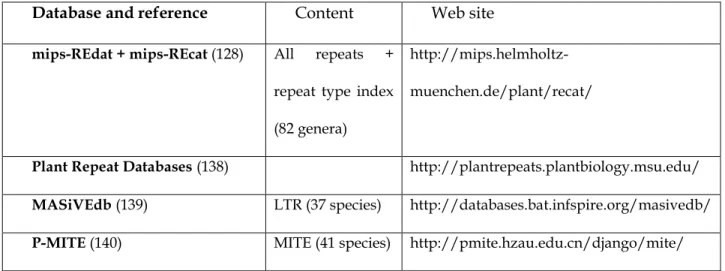
The most common approach used to detect TEs is by homology to already-known TE sequences. This means that the search starts from an existing database of identified TE families and new elements are classified in the family containing the most similar sequence. In practice, this is often done on protein coding sequences (e.g. reverse transcriptase) since reaching a significant level of similarity requires a sufficient conservation level throughout evolution. In all cases, it assumes that a database of known TEs is available. A well-known generic database for eukaryotic consensus repeated sequence models is Repbase Update (6), maintained by the Genetic Information Research Institute (GIRI, Mountain View, CA). The current version, at the date of this publication (Jul. 2014), contained 8,300 loci related to the Viridiplantae clade. Some more specific databases exist. In Table 1, we list a few plant transposable element databases that cover several plant genera. Two of them cover all kinds of repeats that can appear in genomes, the most complete to date being mips-REdat.
A second approach for detecting TEs, called structure-based (7), tries to be less dependent on known sequences by taking advantage of a priori knowledge of
characteristic features of transposon families. For instance, LTR sequences have been analyzed for more than twenty years and a number of common elements have been discovered in their architecture: a short direct repeat string marking the insertion and flanking the 5' and 3' extremities of the LTR, a similar TG..CA box at each extremity, a polypurine tract about 12 bp in length, and various protein domains. All these features can serve as specific constraints enabling the detection of new elements in genomes. They usually form the basis of specific programs or scripts. We will see in the last section that this constrain solving problem may also be seen as an instance of a general pattern-matching issue, which could be treated by generic programs (parsers).
The most complex approach for detecting TEs is ab initio, without any assumption of the type of transposon being looked for. Typically, this is used at large scale to annotate new genomes. For this reason, ab initio methods make use of the most advanced data structures and string algorithms.
Of course, it is sometimes difficult to clearly state the status of a particular method, which may incorporate several steps belonging to different approaches, for instance, ab
initio and by homology. We have created a fourth category, pipeline, to account for
these more complex frameworks which implement a workflow combining existing software components with their own specific glue code and possibly new contributions.
Most detection methods are listed on the Bergman website1. Previous reviews
classified the software according to the detection method (7) rather than detected transposable element superfamilies. This is a valuable approach for Bioinformatics and for whole-genome annotation and we start with a comprehensive subsection on this issue of systematic TE search in a newly-sequenced genome. Since biologists are often primarily interested in certain TE superfamilies, looking at methods as a second step, we propose, in the remaining subsections, different algorithms targeting specific transposable element (TE) families and then subdividing their presentation by the method itself (ab initio, homology-based, structured and pipeline methods). Our chapter focuses on software that is currently available via code downloading, a website or by email. For each TE class and each type of method, a table summarizes the corresponding list of software and provides for each a reference, a download site and installation requirements.
2.1. Large-scale search of transposable elements
First, we present tools that detect all TE superfamilies. These methods correspond to the majority of the TE detection tools. They generally use sophisticated algorithms to ensure an efficient search of elements and the interested reader is referred to Section 3 for having more details on the way it works on computers and having the possibility to compare related techniques.
All TEs; ab initio methods
Available ab initio methods are listed in Table 2. They can be roughly split into two categories: methods that detect exact repeats of fixed size and assemble or extend them, and methods that directly detect non-exact repeats.
Except for Tallymer (8) and RepARK which detect a range of exact repeats, all methods in the first group detect exact repeats of length k called k-mers. These repeats are stored in various data structures offering a tradeoff between the required amount of memory and the amount of computation. These repeats are stored in various data structures offering a tradeoff between the needed amount of memory and the amount of computation. Reputer (9) and RepeatFinder (10) use the suffix tree data structure for storing and retrieving k-mers, while Tallymer (8) uses the more compact suffix array
data structure. A number of methods such as WindowMasker (11) use a structure that does use the fact that elements are strings, a hash index (not to be confused with h-index… !). RepARK counts k-mers up to k=31, making use of the Jellyfish software (12), which is based on a multithreaded, lock-free hash index. PClouds (13) uses a bit array and a hash index. A software such as RepSeek (14) uses a lower and an upper bound for
k and keeps only the maximal repeats, those that cannot be extended without losing an
occurrence.
Available software solutions offer various alternatives regarding the choice of k, some more practical than others depending on the data set: it is most often a parameter whose value has to be user-provided (ReAS, Repseek, REPuter and RepeatScout); it equals log4(n)+1 for PClouds (where n is the sequence size); it is the smallest integer that
satisfies the equation n/4k < 5 for WindowMasker. In the case of Tallymer, it is an
optimal value calculated from a user-provided range fixing the minimal and maximal values. To be more precise, Tallymer calculates this value from the uniqueness ratio, which is the ratio of k-mers occurring exactly once relative to the total number of k-mers in the genomic sequence. Then the selected k corresponds to the least value where the ratio does not increase significantly with the increase of k (inflection point in the uniqueness ratio graph). All repeats greater than k are written out by Tallymer. RepARK assumes a Poisson distribution for the k-mers unique in the whole genome
and thus determines a frequency threshold to filter significant k-mers that occur at least twice in the genome.
Unlike other methods that detect repeats on genomic sequences, ReAS and RBR work on Whole Genome Shotgun (WGS) and Expressed Sequence Tags (EST) data respectively. ReAS selects WGS that contains k-mers with a high copy number and divides them into 100-bp segments centered on that k-mer. ReAS clusters the WGS containing the same k-mers and creates the consensus sequence of the 100-bp segments. In the RBR method, k-mers are considered as repeats if their frequency is higher than a calculated threshold based on a binomial distribution model.
The next important feature for comparing these tools is the way they build approximated repeats from exact ones. Dynamic programming is a widely used method for this purpose, although it is not the only one and the way it is applied may vary.
Tools such as REPuter, RepSeek and RepeatScout use k-mers as seeds and try to
extend them on both sides. REPuter allows a fixed number of mismatches and uses a
dynamic programming algorithm. For each repeat found, an E-value score is computed using the Kurtz and Myers procedure (15) which corresponds to the significance of mismatch repeats. REPuter also possesses a graphical interface to display the position of copy pairs along the genome, something that may help provide a global view of
duplicated material between chromosomes. RepSeek also extends the k-mer seeds by a dynamic programming approach but accepts more errors (substitutions or indels). Finally, RepSeek calculates for each extended repeat a score based on its length and nucleotide composition. The probability for a given repeat score is computed by estimating the probability P(Sbest_repeat ≥ S) that the scoreof the best local alignment observed between two random sequences of fixed size is larger than a given score S and is expressed as a function of the sequence length and the GC ratio. A minimum threshold score is derived from this probability above which no repeats are expected to be found in random sequences and only repeats with a score higher than this threshold are kept. RepeatScout uses a greedy algorithm to extend the exact repeat to the right and to the left and build a consensus. For each extended nucleotide, the algorithm calculates a score that is computed by summing up local similarities of each sequence with the consensus and uses an incomplete-fit penalty for sequences that partially match the consensus. The extension is stopped when the algorithm finds a locally optimal value value that does not increase after a fixed number of steps (100 by default). RepARK uses a de Bruijn graph assembler for NGS data, Velvet (16), to get the repeat library.
The previous strategy can be enhanced by specific preprocessing treatments. PClouds first excludes tandem repeats. It then clusters similar k-mers (called 'P-cloud
Another approach considers that every relevant approximate repeat is made of a
mosaic of exact repeats. RepeatFinder merges exact repeat pairs if the gap distance
between the repeats is smaller than the maximal allowed gap size (a user parameter to be defined in the command line), or if one repeat overlaps another by more than 75%. RepeatFinder then clusters the merged repeats that have a same maximal repeat or a common hit with an E-value lower than a user-specified parameter, using WU-BLAST (17).
ReAS starts from the consensus sequence of 100-bp segments built on WGS clusters containing the same k-mers. The ReAS algorithm recursively extends the consensus sequence to the left or/and to the right if another 100-bp consensus sequence overlaps it.
Finally, WindowMasker (11) aims solely to mask low complexity regions and repeats in genomic sequences and it does not attempt to annotate or classify them. WindowMasker screens the sequence twice for processing repeats: the first screen computes the frequency of each k-mer (for the direct and reverse strands) and defines several thresholds corresponding to various percentiles of the empirical cumulative distribution of repeat occurrences; the second screen uses a frequency-based score and masks mers whose score exceeds the 99.5% percentile or is between two masked k-mers and has a score exceeding the 99% percentile.
In the second group of ab initio methods, no index is built and repeats are directly detected through the self-alignment of genomic sequences. These methods are thus heavily reliant on dynamic programming and their sensitivity depends on the way in which significant aligned pairs are filtered. PILER (18) and RECON (19) proceed by first aligning each sequence against itself and then, in a second step, selecting repeats that present a high copy number or a score higher than a fixed threshold.
In more detail, RECON 1) creates a graph G(V,E) such that vertices V correspond to subsequences involved in WU-BLAST pairwise alignments and edges E represent overlapping vertices in a global alignment; 2) removes from this graph sequences that do not overlap a significant number of times with sequences belonging to the same cluster of sequences; 3) groups elements that belong to the same repeat family. RECON then creates a new graph H(V',E') for each family such that a vertex V' corresponds to a RECON element and each edge E' corresponds to the overlap between two elements in a global alignment. A RECON repeat family is attributed to each repeat position in genomic sequences.
From the alignment, PILER defines a pile as a list of pairwise hits covering a contiguous region in sequences. PILER saves only hits that cluster with more than p instances (p is a user-defined parameter). An interesting original feature of PILER is that it distinguishes different categories of repeats that correspond to different pairwise hit definitions (or repeat builds) and implements a specific method for each category. Thus,
PILER-DF looks for intact transposable elements and aligns at least three similar piles (not hits) to create a repeat, with this pile alignment avoiding generating fragmented sequences. PILER-TR searches TEs with terminal repeats (LTR retrotransposon) and aligns banded hits (i.e. hits separated by a maximum distance) to create the repeats.
AAARF (Assisted Automated Assembler of Repeat Families (20)) is a simple Perl
script (downloadable at aaarf.sourceforge.net/) that is representative of methods oriented towards the use of incomplete genomic information collected through large sets of reads. It has been tested with success on the maize genome, either with a sample of the TIGR Sanger reads (780 bp on average) or with simulated 454 reads (100 bp on average). It is most useful for trying to detect repeats from the short 454 reads, a widespread situation for biological labs. It is possible to tune a number of parameters using BLAST (21) and ClustalW. Of course, it has some limitations since it is a purely de novo method working on highly fragmented data and it should be used with care particularly when discriminating families of degenerated repeats, such as a series of tandem repeats or a mix of non-autonomous and autonomous transposable elements.
All TEs; Homology-based methods
Available homology-based methods are listed in Table 3. Most of them make direct use of the BLAST software (Altschul et al., 1990) and a BLAST-parser. Currently, these
methods used three BLAST versions: AB-BLAST (22), NCBI-BLAST (21) and PSI-BLAST (23). The BLAST method is a famous and widely-used seed-based approach that looks for the presence of a query from its k-mers and estimates a E-value for the significance of matches. Its principles are recapped in Section 3. For all homology-based methods, the query sequence is a library of consensus sequences from TE copies.
AB-BLAST is the new and commercial version of WU-BLAST (no longer supported)
and is only free in a limited version available to academic users. The input and output files and the binary names are identical to WU-BLAST. Because there are so far no papers published and no source code, it is not possible to describe the algorithm of this new version in further detail. NCBI-BLAST is a widely-used BLAST algorithm variation. By default, k is set to 11 for the DNA (or RNA) and to 3 for the proteins. PSI-BLAST is another version from the NCBI laboratory which is much more sensitive in picking up distant evolutionary relationships than a standard protein-protein BLAST (23).
A BLAST parser is a method that reads the BLAST hits and tries to assemble them to obtain summarized results. Since large scale analysis may produce an amount of results that can reach the amount of input sequences, such a component has a decisive role in practice. It determines the type of annotations that can be expected as a result. The language used to program the parser is an indication of its type of usage: Censor (24), RepeatMasker (25; 26), TESeeker (27), TransposonPSI (28) and RelocaTE (29) are written in Perl and are routines that can be included in more complex workflows; TARGeT (30)
is written in PHP as is intended for use only via a website. Note that, independently of languages, and perhaps because it may be a tedious task for biologists, some authors give only a very brief account or do not write out their algorithm in the corresponding paper, something that is not favorable for the interpretation of results and rational improvement of software by the community. For example, the authors of RepeatMasker did not write a paper about it, although it is possibly the most widely-used software for TE detection. TransposonPSI includes a library of ORFs coding for transposon proteins and uses PSI-BLAST to detect intact coding TEs and TBLAST for slightly degenerated coding TEs.
To be more precise, TARGeT (Tree Analysis of Related Genes and Transposons) is a webserver that does not only detect TEs in genomic sequences but also establishes a phylogeny of these elements. It first uses NCBI-BLAST to find the TE copies, aligns them with MUSCLE (31) and determines consensus with the TE family. Finally, it launches FastTree (32) to create the phylogenetic tree of the TE copies. Censor is a BLAST-parser that can use AB-BLAST or NCBI-BLAST. Censor first launches DUST and NSEQ to remove the micro- and mini-satellites from the genomic sequences. From the BLAST hit positions, it tries to assemble them based on the TE consensus families available in the RepBase database. Censor finally calculates for each match the new similarity score and a hit score. The software TESeeker detects preferentially autonomous and complete transposable elements, in three steps. In the first step,
TESeeker uses NCBI-BLAST to find the partial hits of the transposable element copies, assembles them using CAP3 (33) and creates new consensus using ClustalW (34). Hits with E-values higher than 1x10-20 are eliminated. In the second and third steps,
TESeeker iterates the same method with NCBI-BLAST, CAP3 and ClustalW, but starting from the TE consensus library created during the previous step. RelocaTE is a list of Perl scripts aiming at the identification of given reference TE in NGS short reads (paired or unpaired). It produces the locations of TE insertions that are either polymorphic or shared between the reference and short reads. The identification is based on three tools, BLAT, Bowtie and SAMtools. RelocaTE has been used to characterize the amplification of mPing in Oryza sativa (29).
Like Censor, RepeatMasker first detects and removes the micro- and mini-satellites, by applying Tandem Repeat Finder (TRF) (35). RepeatMasker is very flexible and can launch many BLAST-like software solutions: cross-match (36), NCBI-BLAST (21), AB-BLAST (22), or Decypher (37). The NCBI laboratory has made available a special AB-BLAST version for RepeatMasker called RM-BLAST (38). RepeatMasker identifies the TE superfamily of the fragmented BLAST-like hits and assembles them using methods tailored to each superfamily.
RepeatMasker is a base component used in many applications. There are (at least) four other methods that read the RepeatMasker hit outputs and re-assemble them: Process_hits (39), REannotate (40), RepeatRunner (41) and One code to find them all
(42). Process_hits, a Perl script that can also read a BLAST output, processes a refined output using various formats depending on the user parameters. REannotate defragments RepeatMasker outputs following certain rules: the two fragmented hits have the same orientation; the distance between the first and the last fragment must not exceed a user-specified parameter (default 40kb), and the overlap between two fragmented hits must exceed 10% of the reference length sequence. RepeatRunner, written in Perl, mainly detects the autonomous transposable elements (those that contain an ORF). RepeatRunner first launches BLASTX (22) and RepeatMasker, merges the results of both in a XML-based output and eventually masks the repeats in the input genomic sequence (like RepeatMasker). One code to find them all assemble RepeatMasker hits into complete copies, retrieve corresponding TE sequences and flanking sequences, and compute summary statistics for each TE family.
We end with three other methods that do not use BLAST-like output to detect transposable elements but can nevertheless be related to the homology-based methods, RetroSeq, T-lex and HMMER.
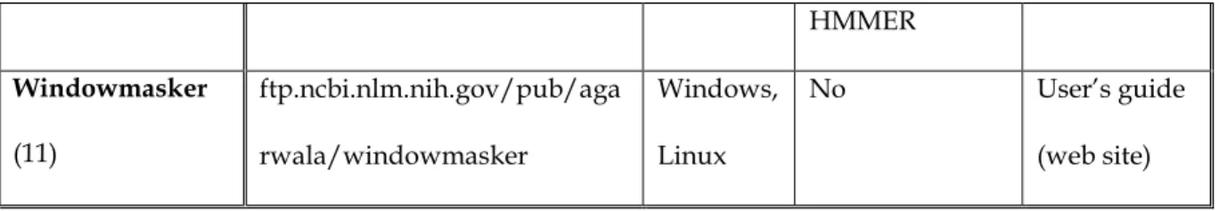
RetroSeq (43) and T-lex (44) detect TEs in next-generation sequencing (NGS) reads and
are described for this reason in Subsection 3.3. HMMER (45) is a widely-used pattern-matching and discovery software package which creates and searches profile Hidden Markov Models (profile HMMs) against a sequence. It was not specifically designed for
TE detection. Three steps are involved in looking for a transposable element belonging to a fixed family using HMMER. One must first align the known copies of the TE family (HMMalign) and then create the HMM profile of this family (HMMbuild and HMMcalibrate). The final step consists in scanning the genomic sequence with the HMM profile as a model (HMMsearch).
All TEs; Structured methods
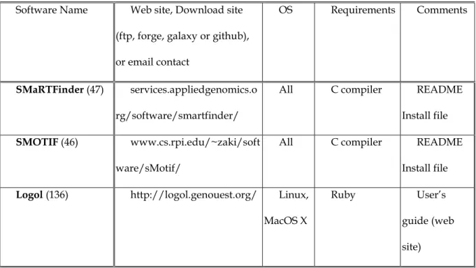
To our knowledge, three structured methods have been applied to detect transposable elements, SMaRTFinder and SMOTIF for the Copia retrotransposons in A. thaliana (also with SMaRTFinder) and STAN used for Helitrons in A. thaliana. This is the reason for citing them here although these methods are not dedicated to the recognition of transposable elements. The corresponding tools are listed in Table 4. They are generic and can be used to detect any biological pattern. This is the subject of Section 4.2, where more complete parsers such as Vmatch are described.
Apart from SMOTIF (46) , SMaRTFinder (47) and Stan (48) use the suffix-tree data structure. SMaRTFinder and SMOTIF first detect all positions of each element of the motif and join the positions that satisfy the distance between the elements of the motif. STAN, on the other hand, creates a list of the possible sequences from the user motif and looks for each of them. Only STAN can detect motifs with substitution errors and
non-fixed gaps. STAN is no longer maintained and a more expressive tool, Logol, can be used instead. It is also described in Section 4.2.
All TEs; Pipeline methods
We end this section with the most elaborate tools, which chain several methods to enhance the repeat annotations and are listed in Table 5. Apart from DAWGPAWS (49), which uses the three kinds of method, RepeatModeler (25), REPET (50), TriAnnot (51) and RISCI (52) use de novo and homology-based methods to detect TEs. All these programs are meta-tools: they launch other software and assemble and rewrite their results. Among TE detection software, only RepeatMasker (26) is used by all these pipelines.
In more detail, DAWGPAWS, written in PERL, launches LTR_STRUCT (53), LTR_seq (54), LTR_FINDER (55), FINDMITE (56), Find_LTR (57), TRF (35), Repseek (14), RepeatMasker, HMMER, TE_Nest (58), and BLAST. DAWGPAWS assembles and rewrites the output of these tools. After removing the tandem repeats with TRF (35),
RepeatModeler, also written in PERL, uses first RECON (19) and RepeatScout (59).
Finally, RepeatModeler launches after RepeatMasker with a library of consensus sequences to identify and assembles the previously detected hits. REPET is a sophisticated method composed of two main pipelines. The first pipeline (de novo) compares the genome against itself using BLASTER (a BLAST-like method written by
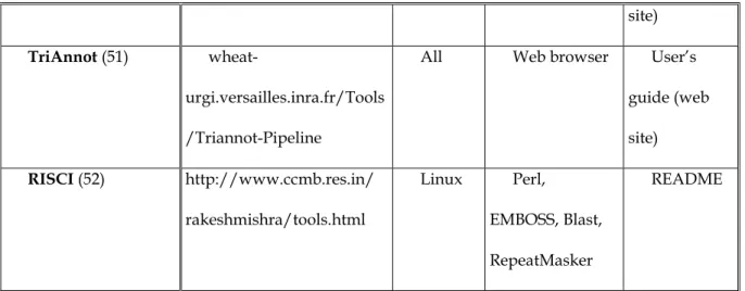
the authors (60)). Then, hits are clustered with RECON, PILER (18) and GROUPER (also written by these authors (60)). A consensus sequence is created by multiple alignment [MAFFT (61) and MAP (62)] and then classified. The second pipeline (homology-based) looks for repeats using a library of sequences, for example the created consensus, with RepeatMasker, CENSOR (24) or BLASTER (60). This pipeline also uses TRF and mreps (63) to detect micro- and mini-satellites. TriAnnot (51) is an annotation pipeline which first detects transposable elements and then predicts the other genetic elements. It launches BLASTX (21), RepeatMasker, TEAnnot (50) (homology-based), and Tallymer (8) (ab initio method). Finally, RISCI (Repeat Induced Sequence Changes Identifier) is a set of Perl scripts specialized in the comparative genomics of transposons. Starting from a reference genome and comparative genomes, it is able to infer intra-species and inter-species structural variations introduced by transposons (e.g. Target Site duplication, inversion and truncation of repeat sequence or post insertion modifications like disruption) . This pipeline uses RepeatMasker, Blast and the EMBOSS module and the Genbank annotation file if made available.
2.2. LTR retrotransposons
Concerning the search and analysis of specific transposable elements, LTR retrotransposons (LTRR) form a large family and offer a rich structure that justifies the
existence of several dedicated tools. An overview of the most interesting ones is provided in Table 6.
Homology-based methods
LTR_MINER (64), written in Perl, is the only homology-based method specialized in
LTR retrotransposon detection. It launches first RepeatMasker and WU-BLAST, and then assembles the multiple hits of the Long Terminal Repeat (LTR) (e.g. the extremities of the retrotransposon) under some constraints: a maximal distance between hits (550 bp), a common orientation, a same LTRR family, and a combined length no larger than a complete LTRR. LTR_MINER also gives information about the probable age of the LTR retrotransposon insertion.
Structure-based methods
LTR_FINDER (55) and LTRharvest (65) detect only full length LTR retrotransposons while LTR_STRUC (53) and MGEScan-LTR (57) detect all LTRs. Aside from LTR_STRUC, LTR_FINDER, LTRharvest and MGEScan-LTR use the suffix-array data structure to find the exact maximal repeats in the genome, and extend/merge them into non-exact repeats. The three methods look also for LTRR signals such as Target Site Duplication (TSD) and PBS and PPT retrotransposon motifs.
In more detail, LTR_FINDER (55) is a web server that merges exact repeat pairs with a similarity score higher than a minimum extension threshold. LTR_FINDER combines dynamic programming (Smith-Waterman algorithm) and the search of structured motifs like the TG..CA box and TSD, in order to adjust LTRR candidate extremities. Next, LTR_FINDER looks for LTRR motifs such as the PBS and PPT signals (by aligning the LTR retrotransposon candidate with the 3' tail of tRNAs) or LTRR protein motifs (using ScanProsite on protein domains such as IN and RH). LTRharvest first builds the suffix array of the genomic sequence using GenomeTools (66) and stores all maximal repeats that are longer than a user-defined threshold. Optionally, LTRharvest looks for motifs such as the TSDs, which can be derived from the maximal repeat occurrences, and the palindromic LTR motif, which corresponds to the dinucleotide palindrome in the LTR extremities (often TG with CA). Finally, LTRharvest checks candidates that have the TSD site, together with some constraints on the size and similarity of the two LTRs and the distance between them. LTR_STRUC, written in C++, first identifies similar pairs subject to a set of constraints: common matching size (larger than 40 bp), similarity (higher than 70%), and distance (lower than a user-defined parameter value). In a second step, LTR_STRUC tries to extend from the initial pair to a second pair in the 3' direction, then the 5’ direction. The extension proceeds by looking in neighboring regions of fixed size (100 bp) for a largest match pair that can be aligned at similar distances from the previous ones and greedily produces the alignment of the whole region by filling the gap by largest matches. This extension process continues until the
similarity falls consistently below the 70% threshold. A last step determines progressively the exact termini of the LTR retrotransposon by calculating the number of matches in a sliding window. Finally, MGEScan-LTR (57), written in C++ and Perl, uses an algorithm similar to LTR_seq (54) (not available) and LTR_STRUC. In a first step, MGEScan-LTR finds all maximal repeat pairs longer than 40 bp and within a range of distances (between 1000 and 20000 bp). Two exact pairs are merged if they are close (less than 20 bp) and share a similarity greater than 80%. In a second step, the method scans the ORFs inside the LTR candidates using HMMER (45), and removes the candidates that match with DNA transposons. In the third step, MGEScan-LTR looks for solo LTRs. It clusters the LTR discovered previously and aligns them to create a profile HMM of each cluster. HMMsearch, a procedure of HMMER, is used to discover these solo LTR retrotransposons.
Pipeline methods
MASiVE (67), written in Perl, is typical of the methods based on carefully designed specific models: it only detects full autonomous LTR of the plant-specific Sireviruses and takes advantage of the highly conserved motifs they share for a sensitive and accurate search. It uses Vmatch (68) - see Section 4.2 - to detect clusters of Sirevirus-specific PPT motifs, and LTRharvest (65) - see Structured methods - to detect complete LTR retrotransposons. Only candidates that possess both hits, the right PBS site, an
admissible distance between the different elements and include LTRS and an internal sequence longer than 500 bp are retained. Wise2 (69) – see Homology-based methods - is used to detect the reverse transcriptase (RT) present in almost intact LTR retrotransposon.
2.3. Non-LTR retrotransposons
The two methods that detect non-LTR retrotransposons first launch homology-based tools, via Perl language scripts, and also look for non-LTR motifs to confirm the TE candidates. They are listed in Table 7.
MGEScan-nonLTR (70) uses dedicated HMM profiles and the pHMM module from
the HMMER package (45) to detect autonomous non-LTR retrotransposons. These profiles correspond to the apurinic/apyrimidinic endonuclease APE, the linker and the Reverse Transcriptase protein domains. MGEScan-nonLTR then classifies the candidates into one of the 12 known non-LTR clades.
RTAnalyzer (71) launches BLAST to detect all non-LTR matches (autonomous and
non-autonomous). From the hits, RTAnalyzer launches Matcher (72), which determines precisely the 5' extremity of the non-LTR retrotransposon. From the corresponding 5' Target Site Duplication (TSD), the algorithm extracts the 3' TSD. Finally, RTAnalyzer
determines the polyA tail, calculates a score from all these motifs and saves the non-LTR candidates that have a score higher than a threshold.
2.4. DNA transposons
DNA transposons are made of a transposase gene flanked by Terminal Inverted Repeats (TIRs) that make structure-based methods the best adapted for an efficient search. The main difference between methods is the way in which TIRs are selected. All methods are listed in Table 8.
Homology-based methods
To our knowledge, there exists only one method specialized in homology-based detection of DNA transposons : TRANSPO (73). It implements a fast bit-vector dynamic programming algorithm (74) that finds the position of all matches similar to a given sequence in a library. The set of matches are then clustered using the SPAT program (75).
Structure-based methods
Five methods use the palindromic structure of their 5' and 3' extremities to detect DNA transposons: Inverted Repeats Finder (IRF) (76), MITE Uncovering SysTem
(MUST) (77), Repetitive Sequence with Precise Boundaries (RSPB) (78), MITE-HUNTER (79) and MITE Digger (80). They all look first for the Terminal Inverted Repeat (TIR), and all but IRF also look for the TSDs that flank the TIR, created during the insertion of the element by a staggered cut in the target DNA.
In more detail, IRF searches TIR candidates that contain exact short inverted repeats (4 to 7 nt) that do not overlap, then extends them, calculates an alignment score for a larger palindromic arrangement and saves the candidates that obtain values higher than the thresholds for similarity (70%) and length (25 bp). MUST detects the TIR associated with the TSD (the minimal and the maximal length of TIR and TSD are user-defined parameters) from a sliding window (up to 500 bp). Candidates with a score higher than a similarity threshold are conserved. MUST then clusters them using the MCL algorithm (81) and writes out the MITE families that contain at least 3 occurrences.
RPBS is a series of Perl scripts using a Blastn-based approach. It seems to have been
essentially applied to non-autonomous transposons of the Miniature Inverted Transposable Elements family (MITE), but the core of its approach could be applied to a broader set of families. The principle is to build clusters of repeats (at least 5 elements, less than 1500 bp) sharing high similarity (Evalue < 10−15) and having precise
boundaries (maximum 5 bp variation and dissimilar 100-bp flanking sequences <50% identity). This software is known to be resource-intensive (several days of computations for large genomes). MITE-HUNTER and MITE Digger have been designed exclusively
to detect MITEs. In MITE-HUNTER, MITE candidates (with their flanking regions) are compared with each other by BLAST (21), and MITE candidates that have similar flanking regions are considered to be part of a larger repeat element and are removed. MITE-HUNTER clusters the remaining candidates and defines a representative element (exemplar) for each cluster (an element that has the greatest similarity with all other elements). BLAST is used to detect its homologs in the input sequences. Candidates that have many copies are then aligned. Homologs such that flanking regions of the MITE sequences are similar (>60%) for the majority of occurrences are assumed to be false positive and discarded. The TSD is predicted again for the remaining candidates for better accuracy. The program creates a consensus sequence from the clustered homologs, compares all consensuses (using BLAST) and clusters them again in order to reduce the number of clusters. MITE Digger is another BLAST-based program designed to scale large genomes by making use of the fact that a MITE family typically contains several hundred highly similar copies that are scattered all over the genome. Rather than repeating for each copy TIR and TSD signature identification, screening, multiple sequence alignment and clustering, the search is first focused on a small portion of the genome and a possible family is filtered out as soon as the number of found copies reaches a threshold. For instance, the probability is very low (1%) of missing 50 copies in 8% of a genome database. Low-complexity regions and hits with very similar flanking regions are discarded from sequences and the process is iterated.
2.5. Helitrons
There seems to be only one method to date specializing in helitron search: HelSearch (see table ) (82) (see Table 9). This is based on the search for a helitron signature in the 5' and 3' extremities. HelSearch looks for the CT[AG][AG]T motif (3' termini) of the helitrons and the small hairpin structure (a 3' sub-termini with a GC-rich sequence) calculated using UNAFOLD (83). It then determines the 5' end (which contains the dinucleotide TC) from the multiple alignment of the potential hits. Finally, HelSearch classifies helitrons based on their 3' end similarity and uses BLAST to detect the fragmented helitrons in the input sequences.
3. Efficient search of repeats in genomic sequences
Some common background appears in all the tools we have seen so far: in most cases, even if it seems a little remote from reality, programs are looking first for exact repeats, often referred to as anchor points or seeds. The real, approximated repeats are obtained by extending the search further from these seeds, by introducing elementary operations
enabling the detection of copies with distant contents. Looking for exact and approximated repeats is part of the rich domain of string algorithms. In the most general setting, detecting repeats in genomic sequences, or in any kind of textual sequence, is organized on the basis of the detection of particular words (the queries) in a text (the bank). This setting appears clearly when processing alignments in homology-based methods or looking for particular motifs in structure-homology-based methods.
There are basically two ways of performing such detection.
In the first case, the text is not preprocessed and the query is searched on the fly in the text. For instance, this is the case when using the well-known “Ctrl-F” shortcut key or search function on any piece of software dealing with texts (text editors, web browsers, etc.). Beginning in the early 1970s, there are strong and interesting theories about fast detection on the fly of queries in texts. This is known as string-matching. The naive way to achieve string-matching is to compare at each position in the text the presence of each character of the query, starting from this position. Obviously, if n is the size of the text and m is the size of the query, this would require n.m comparisons. Thinking of large texts (several gigabytes for a genome), and even for relatively small queries (say 1000 bp), this quickly becomes an issue. It is possible to decrease this complexity for a linear behavior, although it will always depend of the size of the bank. We will not address the topic in this chapter but the interested reader can refer to the excellent book from Charras & Lecroq (84), which explores string-matching algorithms exhaustively and in a
didactic way. A more general approach, pattern-matching, is discussed in the last section (linguistic analysis).
Given their huge volume, the treatment of genomic sequences is generally based on the second way of performing text processing: the text is preprocessed by indexation
techniques. In the previous section, many technical terms have been used, such as suffix
trees and suffix arrays. These are structures developed for fast indexation and searching in texts. Research in this area has been fostered by developments in genomics and in Internet content querying and we propose a quick but up-to-date review of the key results achieved to date. We focus on indexing techniques which open the way both to fast queries and to repeat detection.
3.1. The art of indexing
Imagine what would happen without indexation while looking, for example, for a word (query) on the Internet (bank). Your favorite search engine would open and then read all words of all pages of the whole web in order to detect the presence/absence of your query in each page. Estimated to a few tens or hundreds of billions of webpages, querying the web would simply be impossible, whatever the computation resources available. The same would be the case if the bank is a large set of genomic sequences, such as Genbank. For an efficient search, indexes are necessary. An index is a mechanism that can answer the question: “where does this word occur in the bank?”
within an amount of time that does not depend on the size of the bank. To be precise, indexes are built once for a given bank (and within a time proportional to the size of the bank) and then the time it takes to perform every query in the bank depends only on the query size. Happily, indexes also have “side effects” which are valuable in the biological context, such as the efficient detection of repeats inside or between genomes.
The main idea is to use data-structures to organize and structure the information initially present in the banks. A classic and well-known structure is the dictionary: searching for a word in a paper dictionary does not require reading the entire book, as words are organized in lexicographic order. Similarly, the data-structures used for indexing texts are computational objects having the same advantages as classic dictionaries: they enable a portion of a sequence to be searched quickly by avoiding all portions where this query could not occur. However, while genomes can easily be seen as particular texts, the notion of “word” is not natural in this context since no general delimiter exists. This is why indexes used in this context are designed to answer questions regarding any word in the bank. For example, consider a sequence
S=ATGCGCAGTTTAT as a bank, and a query P=GCGC: “does P occurs somewhere in S, and, if yes, where?” In this example the answer would be “P occurs at position 3 in S”. From the point of view of strings, positions are associated to suffixes of the text, that is, words starting at this position and ending at the end of the text. For instance, position 3 in S is associated with the word GCGCAGTTTAT (and P is a prefix of this word, that is, it is
placed at its beginning). There are a number of indexes primarily powered by this
important notion of the suffix: automaton, hash tables, suffix trees or suffix arrays. All of these data-structures are designed to answer at least the fundamental question “where does P occur in S?”, but each has some specific skills either in terms of additional possibilities or in terms of performance (time efficiency and memory footprint).
Here we propose focusing on the most well-known and most widely-used data-structures: suffix trees, an “historical” data-structure which is no longer extensively applied in practice but which, in addition to useful educational and theoretical properties, also affords the most and the most flexible functionalities; suffix arrays, an efficient and elegant way to index large datasets and answer additional useful questions such as those related to exact repeats in a bank; and, lastly, the Burrows-Wheeler
transform on which the compressed FM-index is based and which is a development that
makes it possible to build compressed suffix arrays. Note that in all cases, an efficient program code appears quite short but is in fact very tricky and definitely not within a standard programmer’s reach: use well-written libraries!
Suffix trees
Suffix trees are represented by a classification tree structure that clusters the suffixes of the indexed text. All suffixes having a common prefix are clustered in the same class
under a common internal node that has this prefix as a label. Any suffix can be read along exactly one path from the unique root of the tree to one of its leaves and
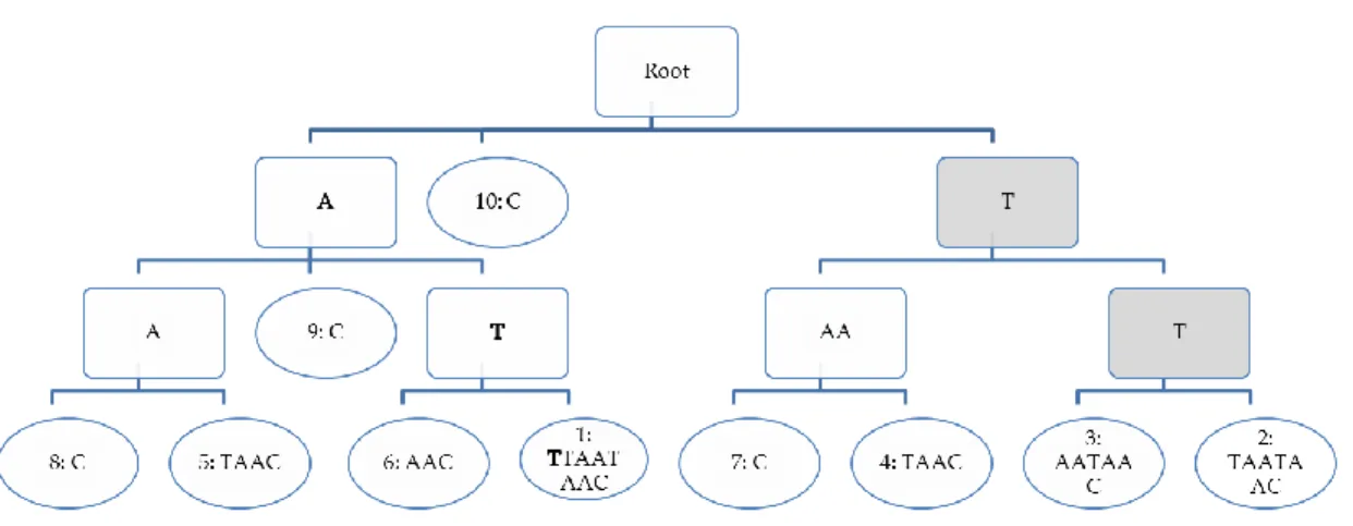
conversely, any path from the root to a leaf corresponds to a unique suffix of the text or, equivalently, to a position in this text. Figure 1 shows an example of the suffix tree of
S=ATTTAATAAC. The suffix at position 8 in the text, AAC, can be read from the root to
the leftmost leaf labeled 8:C by collecting all the words along the path, A, A, and C.
There are strong theories and beautiful algorithms for constructing suffix trees quickly and with the lowest memory requirements. The most famous include the Weiner (85) and later the Ukkonen (86) algorithms which both propose a way of constructing the suffix tree of a sequence composed of n characters with a number of operations and a memory requirement proportional to n. To be precise, storing the suffix tree for a genomic sequence whose alphabet is limited to letters A, C, G and T requires in the worst case 20 bytes per indexed character in optimized applications (87). Indexing the human genome therefore requires 61.47 GB of memory. Even if the actual average amount of memory required is rather around 13 bytes per nucleic acid, storing the suffix tree puts a strain on the main memory for large-scale applications. Applied, for instance, to indexing an Illumina run composed of 100 million reads of length 100 would require 130 GB of memory. In order to save space, it is necessary to shift the space/time tradeoff in the program. One option is to save the tree to hard disk rather
than the main memory but this becomes much slower to access. The most recent implementations of suffix trees have used compressed structures, to the cost of slightly slower access (88). The corresponding program is available in C++ on the website (89).
The suffix tree makes it possible to answer a query in an amount of time proportional to the length of the query. Indeed, any word P read in the tree of an indexed sequence S from its root to any one of its leaves corresponds to a word in S. For instance, searching for the word ATT in the suffix tree of S =ATTTAATAAC can be read in bold in Erreur !
Source du renvoi introuvable. , leading to a leaf labeled 1: ATTTAATAAC meaning that
the word ATT exists at starting position 1 in S.
Fortunately, the suffix tree offers many possibilities other than answering such simple queries. For instance, it is of great interest for detecting exact repeats. Indeed each internal node of the tree (squares in Erreur ! Source du renvoi introuvable.) determines a word which has several occurrences. This is the case for the word TT in our example (path with grey rectangles in the Figure): the corresponding cluster contains leaves labeled 3 and 2, meaning that there are two occurrences of TT in S, starting at positions 2 and 3. Moreover, simple algorithms can exploit the suffix tree to find easily distinct kinds of repeats: those having the maximal number of occurrences, the longest, those that are maximal in their length (adding a new character to the repeat would discard some occurrences), etc. The suffix tree can be applied to more than one unique sequence, in this case it is called a generalized suffix tree. The generalized suffix
tree is useful in genomics as it affords, for example, the possibility of easily determining the words that are copied between different sequences or chromosomes.
Suffix arrays
The suffix array appeared in the early 1990s with the Manber and Myers paper (90). This data-structure is much simpler than the suffix tree, requires less memory space and answers the same range of questions. It is constructed by first sorting all suffixes of the indexed text and by storing the obtained set in alphabetic order, remembering the obtained starting positions.
For instance, the set of suffixes of S=ATTTAATAAC is made of ATTTAATAAC
(starting position 1), TTTAATAAC (pos. 2), TTAATAAC (pos. 3), TAATAAC (pos. 4),
AATAAC (pos. 5), ATAAC (pos. 6), TAAC (pos. 7), AAC (pos. 8), AC (pos. 9), and C (pos. 10). Their alphabetic order is: AAC, AATAAC, AC, ATAAC, ATTTAATAAC, C, TAAC,
TAATAAC, TTAATAAC, and TTTAATAAC. Let us represent this set of suffixes in a table:
Position Suffix 8 AAC 5 AATAAC 9 AC 6 ATAAC 1 ATTTAATAAC 10 C
7 TAAC
4 TAATAAC
3 TTAATAAC
2 TTTAATAAC
The suffix array may be reduced to the Position column of the previous table (the suffixes are represented to promote better understanding of the structure but are never stored in the computer memory). This sole column may appear rather minimalist, but this simple piece of information and the original indexed sequence are sufficient for efficiently answering a query. In its simplest form, it can be found by applying a dichotomic procedure: i) look for the word at the middle position of the array. If the query occurs at this position the search stops, or ii/ if the query is alphabetically smaller than the suffix starting at this position, recursively apply the procedure to the upper part of the array, or apply it to the lower array.
For instance, searching the query Q=AC in the previously indexed text
S=ATTTAATAAC would entail the following steps. First check the middle of the array. In
this example, it corresponds to the suffix at position 1, that is, ATTTAATAAC. As it is alphabetically larger than the query Q=AC, the process restarts with the array limited to:
Position Suffix
5 AATAAC
9 AC
6 ATAAC
Consider the middle line of this array: it corresponds to the suffix starting position 5,
AATAAC, which is alphabetically smaller than the query Q=AC. Thus the process restarts with the lower part of the array. In this case, position 9, where the suffix AC starts, corresponds to the searched query. With this simple procedure, at worse, the number of steps to be performed is log(size of the array) = log(size of the indexed sequence). The query time can be further improved by the use of a new column called the LCP, which provides the length of the “Longest Common Prefix” between two consecutive lines in the suffix array. For instance, if 0 is a LCP default value for the first suffix of the array, the two lines of the previous suffix array would become:
Position LCP Suffix
9 0 AAC
6 2 AATAAC
The value 2 indicates that AAC and AATAAC start with 2 common characters. The
LCP somehow enables retrieval of the suffix tree topology, and then enables answering questions related to repeats. In the example, LCP =2 indicates that a repeat of size 2 exists in the indexed text, at positions 9 and 6 given by Position.
The suffix array (together with the LCP array) requires (for classic genomic analyses) 5 bytes per indexed character. Thus, indexing a 3.3 billion-character human genome with a suffix array and its LCP would require 15.37GB. The indexation of a hundred million reads of length 100 would require 46.57GB of memory. A good C++ code is available in the appendix of the paper (91) (algorithm DC3) and two other C programs that are among the most advanced implementations to date are given in the appendix of the paper (92) (algorithms SA-IS and SA-DS). We mention the recent paper (93), a didactic presentation of the SA-IS algorithm for Bioinformatics specialists. Regarding access to an operational code in Java, please refer to (94). A recent development in using suffix arrays to look for repeats (finding the largest substring common to a set of sequences and finding maximal repeats exclusive of a sequence with respect to another set of sequences) is described in (95). The C code can be downloaded from (96). In fact, genomic repeats may be a source of inefficiency for certain implementations and care is required when choosing a program. A far more general use of the suffix array data-structure is described in the next section with the software Vmatch (68).
FM-index and Burrows-Wheeler transform
The Burrows-Wheeler transform (97), inspired by the suffix array, was the starting point of the FM-index (98) (99), a new powerful indexing approach that is now widely used in many fields, in particular in computational biology. The Burrows-Wheeler transform (BWT) is a permutation of characters in a sequence that is easy to understand from a suffix array. Using our previous example, ATTTAATAAC, it is the sequence
TTAACAATTA, which can be displayed next to the suffix array as follows:
Position Suffix BWT 8 AAC T 5 AATAAC T 9 AC A 6 ATAAC A 1 ATTTAATAAC C 10 C A 7 TAAC A 4 TAATAAC T 3 TTAATAAC T 2 TTTAATAAC A
For each position in the suffix array, the BWT corresponds to the letter located just before this position in the sequence (or the last letter for position 1). For instance, the letter indicated in the first line is ‘T’ as it is the letter at position 8-1=7 in the text. The
BWT has astonishing properties that we review here briefly. Interested readers can refer
to (97) for further algorithmic details.
A first important property of the BWT is that this permutation (TTAACAATTA in our
example) is reversible: it is sufficient to retrieve the indexed sequence (ATTTAATAAC). This is what is called a self-index, i.e. it is not necessary to keep the indexed sequence in the memory, it is contained in the index.
A second appreciable property of the BWT is that it is highly compressible. Indeed this letter organization tends to create stretches of letters. For instance, consider the sequence “treat peat pea repeats” (spaces added to help reading). Its BWT sequence is “eeeepprprttetataasa”. This is well-suited for compression algorithms (e.g. “eeee” could be rewritten as “4e”).
In 2000, Ferragina and Manzini refined this compression approach to make it capable of answering queries in a text, leading to the FM-index (its full name, “Full-text index in Minute space” does not really help its understanding). To do this, they added a few pieces of information to the BWT while keeping the data structure extremely light. We
cannot enter into the details of this structure, but suffice to know that it can be considered as a kind of compressed suffix array requiring very little memory space. For instance, the human genome could be indexed with this approach using 1.23 GB, and one million reads of length 100 would require 3.73GB of memory. A good source for codes on the FM index and suffix array indexes is the Pizza&Chili reference site (100). The FM-index supports the following operations which generally use a tiny portion of the compressed file:
locate finds the position in the text of an occurrence of the query, in O(logcn) time,
where c is a constant chosen at the time the FM-index is built.
count computes the number of occurrences of the query, in time proportional to
its length;
extract returns the sequence of a given length starting at a given position in the
text;
display outputs for a given length L the L characters on each side of the
occurrences of the query in the text.
Hash tables versus Burrows-Wheeler transform
Another frequently employed indexing data structure is the hash table. The hash table concept stands on a very simple idea. For indexing a set of names for instance, each name is converted into an address (called a hash value) using a function that is
easy to compute. For instance, using a hash function that considers each substring as a number in base 11 (each letter being coded by an ASCII number), "AMY" is given the address 8801=65112+77111+89110 and "BOB" is given the address
8921=66112+79111+66110. In an initially empty array (called the hash table), "AMY"
is stored at position 8801 and "BOB" at position 8921. As it is important to save as much space as possible, it happens that two different names get the same hash value. For instance, imagine now we add the name "AYM" that also has the hash value 8921. This causes a collision at position 8921 that already contains the name "BOB". There are several ways to manage collision, either by computing a new hash value for "AYM" (open addressing) or by storing at each position a list of name (“BOB” and “AYM”). In case of too many collisions, the hash table is overloaded and may be resized. This operation is expensive as it may reorganize all the already stored items.
Querying a hash table is fairly similar to what is done by the indexing algorithm. The hash value of the query is computed, and the content of the hash table at this position is visited in order to check the presence/absence of the queried object. Depending on the strategy used to manage collisions, either all the entries present in the list at this position have to be checked or new hash functions have to be computed for the query until it is found (match) or an empty position is reached (mismatch).
Most programming languages offer simple structures to build hash tables. It is easy to find efficient implementations of hash tables on the web (e.g. SpookyHash (101) or
SparseHash (102)). Some tools implementing hash tables are specifically designed for routine similarity search on NGS data such as RAPSearch2 (103), which allows similarity searches in proteins and is fully compatible with Blast. Implemented in C++, the source code is freely available for download at the RAPSearch2 website (104).
The main advantage of hash tables is their speed, in particular when collisions are absent or rare. Another important advantage stands in the fact that hash tables are dynamic and can host any additional piece of information for each of its items. Unlike the FM-Index, any new item can be added to a hash table, even after its construction. In a biological context, to each k-mer can be associated its list of occurrences in a genome for instance. In comparison, the FM-Index gives only access to the occurring position(s) of each query.
The theoretical indexing and querying times (respectively O(n) and O(m) in average with n being the size of the bank and m the size of the query) are the same for FM-Index and hash table approaches. However, the application range are a bit different. First the hash table contains fixed items. For instance if items are k-mers, a hash table does not allow to query k+1-mer or k-1-mer. Moreover, these items must be explicitly stored. For a human genome, storing 3 billion of 31-mers (coded on a binary alphabet) requires nearly 22 GB of memory. Indexing all 31-mers of a human genome would thus require approximately 23 GB of memory using a hash table (including the array itself). In comparison, the FM-Index is a self-indexed compressed data structure. This means that
the index itself contains the original sequence, and furthermore any k-mer of any size could be queried using this data structure. Indexing a human genome using the FM-index requires less that 2 GB of memory. The BWA methods described in (105) presents in details how the Burrows-Wheeler Transform (BWT) (often simply referred inaccurately as the FM-Index) can be used for performing the mapping of reads on a genome.
All the data structures presented above are designed for exact queries. However they are not made for answering questions such as “where does Q=TAAT occur with at most one error in S=ATTTAATAAC?”. Some attempts to make them able to deal with such requests basically need to enumerate all possibilities. For instance, the previous request would be answered by searching all queries distant by at most one error with respect to Q, representing 4*(size of Q) queries: AAAT, CAAT, GAAT, TAAT, ACAT, etc. If more than one error should be tolerated, then the number of queries to perform explodes, making such solutions inapplicable for biological application. The search for approximated words requires additional techniques, as described in the next subsection.