HAL Id: dumas-01409607
https://dumas.ccsd.cnrs.fr/dumas-01409607
Submitted on 6 Dec 2016HAL is a multi-disciplinary open access archive for the deposit and dissemination of sci-entific research documents, whether they are pub-lished or not. The documents may come from teaching and research institutions in France or abroad, or from public or private research centers.
L’archive ouverte pluridisciplinaire HAL, est destinée au dépôt et à la diffusion de documents scientifiques de niveau recherche, publiés ou non, émanant des établissements d’enseignement et de recherche français ou étrangers, des laboratoires publics ou privés.
Spatio-temporal dynamic of the exploitation of common
sole, Solea solea, in the Eastern English Channel
Hubert Du Pontavice
To cite this version:
Hubert Du Pontavice. Spatio-temporal dynamic of the exploitation of common sole, Solea solea, in the Eastern English Channel. Agronomy. 2016. �dumas-01409607�
Spatio-temporal dynamic of the exploitation of common
sole, Solea solea, in the Eastern English Channel
Par : Hubert DU PONTAVICE
Soutenu à Rennes, le 14/08/2016
Devant le jury composé de :
Président : Etienne RIVOT
Maître de stage : Marie SAVINA-ROLLAND et Youen VERMARD
Enseignant référent : Etienne RIVOT et Didier GASCUEL
Autres membres du jury :
Marianne ROBERT (Chercheur Ifremer Lorient) Verena TRENKEL (Chercheur Ifremer Nantes)
Les analyses et les conclusions de ce travail d'étudiant n'engagent que la responsabilité de son auteur et non celle d’AGROCAMPUS OUEST AGROCAMPUS OUEST CFR Angers CFR Rennes Année universitaire : 2015 - 2016 Spécialité : Agronome
Spécialisation (et option éventuelle) : Sciences Halieutiques et Aquacoles Option REA
Mémoire de Fin d'Études
d’Ingénieur de l’Institut Supérieur des Sciences agronomiques, agroalimentaires, horticoles et du paysage
de Master de l’Institut Supérieur des Sciences agronomiques, agroalimentaires, horticoles et du paysage
d'un autre établissement (étudiant arrivé en M2)
Ce document est soumis aux conditions d’utilisation
«Paternité-Pas d'Utilisation Commerciale-Pas de Modification 4.0 France» disponible en ligne http://creativecommons.org/licenses/by-nc-nd/4.0/deed.fr
Confidentialité
Non Oui si oui : 1 an 5 ans 10 ans
Pendant toute la durée de confidentialité, aucune diffusion du mémoire n’est possible (1).
Date et signature du maître de stage (2) : 04/10/2016
A la fin de la période de confidentialité, sa diffusion est soumise aux règles ci-dessous
(droits d’auteur et autorisation de diffusion par l’enseignant à renseigner).
Droits d’auteur
L’auteur(3) Nom Prénom DU PONTAVICE Hubert
autorise la diffusion de son travail (immédiatement ou à la fin de la période de confidentialité)
Oui Non
Si oui, il autorise
la diffusion papier du mémoire uniquement(4)
la diffusion papier du mémoire et la diffusion électronique du résumé
la diffusion papier et électronique du mémoire (joindre dans ce cas la fiche de conformité du mémoire numérique et le contrat de diffusion)
accepte de placer son mémoire sous licence Creative commons CC-By-Nc-Nd (voir Guide du mémoire Chap 1.4 page 6)
Date et signature de l’auteur : 04/10/2016
Autorisation de diffusion par le responsable de spécialisation ou son
représentant
L’enseignant juge le mémoire de qualité suffisante pour être diffusé (immédiatement ou à la fin de la période de confidentialité)
Oui Non
Si non, seul le titre du mémoire apparaîtra dans les bases de données. Si oui, il autorise
la diffusion papier du mémoire uniquement(4)
la diffusion papier du mémoire et la diffusion électronique du résumé la diffusion papier et électronique du mémoire
Date et signature de l’enseignant :
(1) L’administration, les enseignants et les différents services de documentation d’AGROCAMPUS OUEST s’engagent à respecter cette confidentialité.
(2) Signature et cachet de l’organisme
(3).Auteur = étudiant qui réalise son mémoire de fin d’études
(4) La référence bibliographique (= Nom de l’auteur, titre du mémoire, année de soutenance, diplôme, spécialité et spécialisation/Option)) sera signalée dans les bases de données documentaires sans le résumé
Remerciements
Je tiens, en tout premier lieu, à remercier Marie Savina-Rolland et Youen Vermard, mes encadrants de stage pour leur confiance, leur patience, leurs conseils avisée et leur accompagnement tout au long de ce stage. J’ai pris beaucoup de plaisir à partager ces 6 mois de stage avec vous tant sur le plan scientifique qu’humain. Je tiens également à vous remercier pour votre soutien et vos précieux conseils lors de ma préparation des concours des écoles doctorales.
Je tiens à remercier Paul Marchal et à Bruno Ernande pour leur disponibilité et leurs conseils tout au long de mon stage. Merci à toi Bruno d’avoir pris du temps pour moi et de m’avoir fait bénéficier de tes compétences en statistiques.
Merci également à Etienne Rivot et Didier Gascuel pour le suivi de ce stage et leurs conseils.
Un grand merci aux membres du centre Ifremer de Boulogne-sur-Mer pour m’avoir si bien accueilli et intégré. Je tiens à remercier particulièrement : Charles, Jérémy, Pierre, Khaled, Rémi, Clémence, Cyrielle et Cecilia pour leur bonne humeur, les très bons moments partagés et pour m’avoir prouvé que la vie à Boulogne n’était pas aussi terrible que je l’imaginais. Un grand merci à toi Cecilia (« Miss Rome » pour les intimes) de m’avoir supporté dans ton bureau pendant ces 6 mois de stage. Je vous suis, également, à tous, très reconnaissant de m’avoir soutenu, encouragé et conseillé dans la recherche d’une thèse puis lors de la préparation des concours des écoles doctorales.
Merci aux copains de l’agro, de prépa et d’enfance pour leur soutien et leur amitié.
Je tiens à remercier ma famille et en particulier mes parents et sœurs pour leur soutien perpétuel ; Et enfin merci à Anne qui me supporte et me soutient depuis de nombreuses années.
Abstract
The Eastern English Channel (EEC) common sole (Solea solea) stock is one of the most important stocks for the French fisheries in the EEC. Low recruitments in 2012 and 2013, coupled with a fishing mortality well above Fmsy led to repeated cuts in TAC over the last years. This master thesis aimed to study the spatiotemporal dynamics of the French fisheries exploiting sole in the EEC and their impact on this stock; it also allowed drawing assumptions on populations’ dynamics. We first showed a spatial structuration of the French fisheries (mainly trammel net and bottom otter trawl). A focus on trammel netters which represent the main share of the landings and which are highly dependent on common sole showed spatial differences on the length structures of the catches. Regression trees on mean lengths of catches and a multinomial logistic regression on the length structures of the catches revealed that these differences can be explained by the mesh size used, fishing period and the fishing area (including nursery area). The impact of potential subpopulations with different biological parameters in the EEC was tested focusing on growth parameters in these subareas, using a non-linear mixed effect model. It showed differences in growth rates and asymptotic lengths between the Northeast and the Southwest of the EEC. Finally, differences in the landings were checked through exploitation patterns to describe links and differences between catches and landings in the different regions and areas.
List of Figures
Figure 1: a) Spatial landings distribution by country exploiting common sole in the EEC
between 2010 and 2013; b) Proportion of landing by country exploiting common sole in the EEC between 2010 and 2013. (From CSTEP data) ... 1
Figure 2: Sole in Division 7.d. Summary of stock assessment. a) Stock Size: Spawning Stock
Biomass; b) Fishing Pressure; c) Recruitment for age 1 (ICES, 2016), the white bar represents the predicted recruitment in 2017. ... 2
Figure 3: French landings (in t) of Common Sole in EC by statistics rectangle between 2001
and 2015. ... 5
Figure 4: French landings of common sole in the EEC and quota (before the exchanges
between EU countries) between 2000 and 2015 ... 5
Figure 5: Contribution of the different gears to the French common sole landings in the EEC
in 2015 ... 6
Figure 6: a) Landings by regions and by fishing gear from 2000 to 2015, b) spatial landings
distribution by fishing gear. Pies are proportional to the volume landed in the statistical rectangles. ... 7
Figure 7: Contribution of the different mesh size range for the trammel net to the French
common sole landings in the EEC in 2015. ... 7
Figure 8: Mesh size range proportion in common sole landing in Eastern Channel for 2009,
2011, 2013 and 2015 from the SACROIS database. ... 8
Figure 9: Common sole total landing in the EEC by statistical rectangle and by commercial
category. Pies are proportional to the volume landed in each quarter in the given statistical rectangles. ... 9
Figure 10: Common sole total landing of the trammel netters in the EEC by statistical
rectangle and by commercial category. Pies are proportional to the volume landed in each quarter in the given statistical rectangles. ... 9
Figure 11: Selectivity curves for Solea solea in Basque country using SELECT models;
dashed line: 90mm inner panel mesh, continuous line: 100mm inner panel mesh, bold line: 110mm inner panel mesh (Erzini et al., 2006). ... 11
Figure 12: a) 3 subareas colored in blue, red, and green and the darker areas along the coast
representing the nurseries area; b) Position of trammel net hauls with common sole in the EEC from Obsmer between 2009 and 2015 ... 12
Figure 13: Mean length by statistical rectangles of catches between 2009 and 2015: a) for all
mesh size range, b) only for 90-99mm mesh size range ... 16
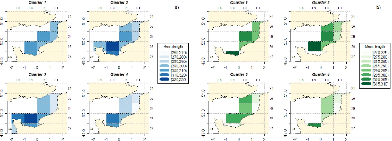
Figure 14: Mean length by statistical rectangle and by quarter of catches between 2009 and
2015: a) for all mesh size range, b) only for 90-99mm mesh size range ... 16
Figure 15: a) Regression tree developed from mesh size, quarter, nursery, and latitude and
longitude. Choosing cuts are indicated on each branch in italics. The mean lengths and the numbers of individuals (combination in our case) are indicated in bold at each leaf at the base of the tree. b) Map of the Eastern Channel, where points represent trammel net hauls for both mesh size ranges and lines represent longitudes highlighted in the 1st regression tree. ... 17
Figure 16: Regression tree developed from mesh size, quarter, nursery and subarea. Choosing
splits are indicated on each branch in italics. The mean lengths and the numbers of individuals (combination in our case) are indicated in bold at each leaf at the base of the tree. ... 18
Figure 17: Residuals of the multinomial regression: observed length distribution - predicted
length ... 18
Figure 18: Predicted and observed length distributions of capture of common sole for two
mesh size ranges 100-119mm and 90-99mm ... 19
Figure 19: Predicted and observed length distribution of capture of common sole for the two
subareas Northeast and Southwest (respectively in blue and in orange) for a) global catch, b) catches with mesh size in the range 90-99mm, and c) catches with mesh size in the range 100-119mm ... 20
Figure 20: Predicted and observed length distributions of capture of common sole in or out
the nursery areas (respectively in red and in green) for a) global catch, b) catches with mesh size range 90-99mm, and c) catches with mesh size range 100-119m ... 20
Figure 21: Length distribution of capture of common sole in or out the nursery areas
(respectively in red and in green) by quarter and by a mesh size range: a) 90-99mm and b) 100-119mm. n(In) and n(out) indicate the number of individual in each length distribution .. 21
Figure 22: Predicted and observed length distribution of capture of common soles by quarter
and by a mesh size range 90-99mm (a) and 100-119mm (b). ... 22
Figure 23: Predicted and observed length distribution of capture of common soles by year
and by a mesh size range 90-99mm (a) and 100-119mm (b). ... 23
Figure 24: At right, the observed length distribution of common soles capture of trammel
netters (90-99mm and 100-119mm) by year between 2009 and 2015 in and out nursery areas (in red and in green, respectively). At left, the Recruitment for age 1 (ICES, 2016). The red arrows indicate the good recruitments and the blue arrows the bad recruitment ... 25
Figure 25: Residuals of the non-linear mixed model; a) Fitted values vs Standardized
residuas; b) QQ plot ... 29
Figure 26: a) Discarded fraction and b) Mean length of the discards of common sole captures
by trammel netters in the EEC by subarea and by year, between 2010 and 2015. ... 32
Figure 27: Sole discards and landings length distribution between 2009 and 2015 in the NE
and in the SW of the EEC for the mesh size ranges 90-99mm and 100-119mm; n(FO) indicate the number of fishing operations used to produce each length distribution and the green line indicates the MLS before 2015 (240mm). ... 32
Figure 28: a) Discarded fraction and b) Mean length of the discards of common sole captures
by trammel netters in the EEC by region and by year, between 2010 and 2015 ... 33 Figure 29: Sole landings and discards length distributions between 2009 and 2015 in Basse-Normandie, Hauts-de-France and Haute-Normandie; the green line indicates the MLS before 2015 (240mm). ... 33
Figure 30: a) Discarded fraction and b) Mean length of the discards of common sole captures
by trammel netters in the EEC by region and by year, between 2010 and 2015. ... 34
Figure 31: Length distribution of captures of common sole between 2009 and 2015 inside
and outside the nursery area for the mesh size range 90-99mm and 100-119mm with the catch category (Discard or landings); n(FO) indicate the number of fishing operation used produce each length distribution and the green line indicates the MLS before 2015 (240mm). ... 34
List of Tables
Table 1: Description of Soles commercial categories ... 4 Table 2: Description of variables used in the statistical analyses: 2 regression trees (RT) and 1
multinomial logistic regression (MLR) ... 13
Table 3: Length classes used for the multinomial logistic regression with the number of
individuals in each class and the corresponding percentage. ... 14
Table 4: Mean value of the growth parameters from the non-linear mixed model between
2010 and 2015 for each combination of Quarter, Subarea and Sex kept in model. In the last column, the percentage of difference was computed between two subareas in the EEC: the Northeast (NE) and the Southwest (SW). ... 30
List of Appendix
Appendix I: Technical description of the main gear exploiting common sole in the Eastern
English Channel ... i
Appendix II: Spatial distribution of common sole landings in the EEC by region in 2015. .... ii Appendix III: a) Relative error and 1-R² as a function of complexity parameter and the size
of the tree; b) Residuals of the 1st regression tree (observed vs. predict values) ... iii
Appendix IV: a) Relative error and 1-R² as a function of complexity parameter and the size
of the tree; b) Residuals of the 1st regression tree (observed vs. predict values) ... iv
Appendix V: analysis of variance of the multinomial logistic regression model ... v Appendix VI: a) Confusion matrix from the cross-validation of the multinomial logistic
regression model, “Prediction” is the predicted length class computed from the model build with the learning sample and “Reference” is the observed value of the validation sample. b) Distribution of the observed length class depending on predicted length class from the cross validation. ... vi
Appendix VII: Length distribution of capture of common sole in SW or NE in the EEC by
quarter and by a mesh size range: a) 90-99mm and b) 100-119mm. ... vii
Appendix VIII: Length distribution of capture of common sole in SW or NE in the EEC by
year and by a mesh size range: a) 90-99mm and b) 100-119mm. ... viii
Appendix IX: Summary of the final model selection with the different models tested. The
procedure began with select random effects and, then fixed effects; the complete model is highlighted in blue and the final model in green. For each effect in the model, 1 is assigned to the growth parameters taken into account in the model and 0 otherwise. P-value is the result of loglikelihood ratio. ... ix
Appendix X: Factorial design on the Year, the Quarter and the Subarea of the Bargeo data . x Appendix XI: Analysis of variance of the non-linear fixed effect model ... xi Appendix XII: Summary of the non-linear mixed effects model with the parameters for the
random effects and for the fixed effects. ... xii
Appendix XIII: Growth curves for computed from K, Linf and L2 estimated in the non-linear
mixed model for female common sole in the EEC depending on the quarter, the year and the subarea: SW in orange and NE in blue The points represent the observed length-at-age from Bargeo data in the SW (orange) and in the NE (blue) ... xiii
Appendix XIV: Growth curves for computed from K, Linf and L estimated in the non-linear
mixed model for male common sole in the EEC depending on the quarter, the year and the subarea: SW in orange and NE in blue The points represent the observed length-at-age from Bargeo data in the SW (orange) and in the NE (blue) ... xiv
Appendix XV: Mean length of common sole in the EEC at each quarter from the age 2 to the
List of Acronyms
AIC: Akaike Information Criterion BN: Basse-Normandie
CC: Commercial Categories HF: Hauts-de-France
HN: Haute-Normandie
EEC: Eastern English Channel FO: Fishing Operation
MLR: Multinomial Logistic Regression MLS: Minimum Landing Size
NE: Northeast RT: Regression Tree SW: Southwest UK: United Kingdom
Tables of contents
1. Introduction & context ... 1
1.1. Biology & ecology ... 1
1.2. Exploitation, assessment and management ... 1
1.3. Anthropic impacts ... 2
1.4. Scientific and socio-economic issues, and problematic ... 3
2. Spatiotemporal dynamics of common sole French landings in the Eastern English Channel ... 3
2.1. Materials & Methods ... 4
2.2. Results ... 5
Spatial distribution of total landings ... 5
2.2.1. Regional landings ... 5
2.2.2. Spatial distribution of landings by fishing gear ... 6
2.2.3. Spatial distribution of landings by mesh size used in the trammel net fishery .... 7
2.2.4. Spatial distribution of landings by commercial category ... 8
2.2.5. 2.3. Discussion ... 10
3. Length structure of common sole captures by trammel nets in the EEC ... 11
3.1. Introduction ... 11
3.2. Materials & Methods ... 12
Data ... 12
3.2.1. Analytical Methods ... 12
3.2.2. 3.3. Results ... 16
Mean length variability ... 16
3.3.1. Length class distribution ... 18
3.3.1. 3.4. Discussion ... 23
Fishing impact – Selectivity ... 23
3.4.1. Impact of structure of population ... 24
3.4.2. Nursery ground ... 24
3.4.3. Temporal variability ... 25
3.4.4. 4. Spatial analysis of growth parameters of common sole in the Eastern English Channel 26 4.1. Materials & Methods ... 26
Data ... 26
4.1.1. Estimation of growth parameters ... 26 4.1.2.
Analytical Method ... 27
4.1.3. 4.2. Results ... 28
4.3. Discussion ... 30
5. From catches to landings ... 31
5.1. Materials & Methods ... 31
Data ... 31
5.1.1. Discarded fraction estimate ... 32
5.1.2. 5.2. Results ... 32
5.3. Discussion ... 35
Conclusions and perspectives ... 36
Bibliography ... 37
Webography ... 39
1
1. Introduction & context
1.1. Biology & ecology
Common sole, Solea solea, is a benthic species living on fine sand and muddy substrates between 0 and 150 metres deep. The biogeographical range of common sole extends, in eastern Atlantic, from southern Norway down to Senegal, and the Mediterranean Sea including the Marmara and Black Seas (Carpentier et al., 2009). Sole feeds on annelid worms, small molluscs and crustaceans (Carpentier et al., 2009). Sole life cycle includes a pelagic larvae stage followed by a benthic juvenile stage in the estuarine and coastal nurseries grounds (Riou et al., 2001). At maturity, young soles (aged 2 and 3-years) move away from coastal area toward deeper grounds and breed every year (Le Pape, 2005). In the Eastern English Channel (EEC), breeding takes place from February to June with a maximum intensity in April/May (Carpentier et al., 2009; Ifremer, 1993).
ICES (ICES, 2015) assumes a single population in the area VIId (ie: the EEC) and sole is assessed and managed as such. However, Rochette et al. (2012) suggested the existence of 3 isolated sub-population at the scale of the EEC. This hypothesis is mainly based on larval dispersion analyses which showed limited dispersion between spawning areas and coastal and estuarine nursery ground (Rochette et al., 2012). In addition, previous analyses showed that sole juveniles stay in their nursery grounds during their 2 first years of life (Coggan and Dando, 1988; Le Pape and Cognez, 2016; Anon, 1989) and remain close to their nursery area even after seasonal spawning migration (Kotthaus, 1963; Anon, 1965). A mark-recapture survey suggested the low mobility of adult soles (Burt and Millner, 2008).
1.2. Exploitation, assessment and management
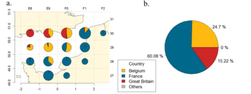
The EEC stock is mainly exploited by three countries, France, Belgium and the United Kingdom. Between 2010 and 2013, UK fleets operated only along the English coast, while Belgian fleet was spread over the Northwest of the (Figure 1, a). They represented, respectively, 15% and 25% of landings of common soles in the EEC (Figure 1, b). French fleets, which gathered 60% of the landings of common soles, were concentrated along the French coast.
Figure 1: a) spatial landings distribution by country exploiting common sole in the EEC between 2010 and 2013; b) Proportion of landing by country exploiting common sole in the EEC between 2010 and 2013. (From CSTEP data)
French fleets exploiting the common sole stock in the EEC is dominated by trammel netters and trawlers. Globally netters exploiting common sole in the EEC are small vessel that fish
2
close to the French coast. The others French fleets exploiting common sole in the EEC are small bottom trawl fleet and polyvalent fishing vessels seasonally targeting sole (pers. comm.).
This stock is considered overfished. From 1980, fishing mortality on this stock has fluctuated at levels higher than Fmsy (ICES, 2016) (Figure 2, b). Low recruitments in 2012 and 2013 (Figure 2, c) and high fishing mortality have led to a deterioration of the stock condition with a declining biomass from 2013. This decrease in biomass induced management measures and TAC cuts since 2014 (ICES, 2016). In 2015, the estimated SSB (Stock Spawning Biomass)
was close to MSY Btrigger (8143 tonnes) and fishing mortality close to the Flim. The aim set by the CFP in 2011 was to achieve Fmsy by 2015, or as soon as possible thereafter. In 2016 ICES advice is therefore based on the MSY approach and recommend to further reduce the TAC by 24% to achieve Fmsy in 2017 (ICES, 2016).
Figure 2: Sole in Division 7.d. Summary of stock assessment. a) Stock Size: Spawning Stock Biomass; b) Fishing Pressure; c) Recruitment for age 1 (ICES, 2016), the white bar represents the predicted recruitment in 2017.
In 2016, a multi-annual management plan was proposed by the NWWAC (North Western Waters Advisory Council) aiming at maintaining the TAC at 3,000 tonnes until 2020 provided that the biomass is maintained above Bmsy-trigger (NWWAC, 2015). Unfortunately, ICES could not consider this plan in the last stock assessment as it had not been officially endorsed by EU.
1.3. Anthropic impacts
The main anthropogenic disturbance is due to overfishing. The direct effects of fishing causes declines of biomass and indirect effects can affect sole populations. Selection pressure by fishing has an impact on growth and, length and age at of exploited species. Mollet et al. (2007) showed, in the North Sea, a decrease in the size of female at age 3 from 286 mm (and 251 g) to 246 mm (and 128 g) between 1960 and 2002. In addition, low mobility might render the quality of the habitat even more important for Sole than for more mobile species. Habitat degradation is one of the most serious threats for the recovery of fish stocks (Jennings and Kaiser, 1998). Nursery habitats, which are an essential habitat for juvenile common sole (Riou et al., 2001), sustain anthropogenic disturbance through pollution and habitat destruction. This degradation was notably showed by Rochette et al. (2010) for the Seine Estuary. In this area the loss in habitat surface combined with habitat degradation led to an important loss in the contribution of the Seine estuary nursery to the whole sole population in the EEC.
3
1.4. Scientific and socio-economic issues, and problematic
Common sole stock in EEC is one of the most commercially important species in this area with commercial catch between 4,000 and 5,000 tonnes. Repeated cuts in TAC are hard to overcome by fishing fleets, particularly when they cannot diversify their activity and mostly rely on a given species. In the last years, the main fleets involved in the sole fishery became very dependent on the sole due to several management measures on historical target species (i.e. the cod recovery plan limited cod exploitation and its targeting and restrictive TAC on rays were set). In 2014, French EEC sole fishery made a turnover of more than €13 000 00 and more than 340 fishing vessels were involved in sole fishery.
In this context, a project funded by France Filière Pêche and led in partnership with, DPMA, CRPM Nord Pas de Calais Picardie, Haute and Basse Normandie, the producer’s organisations FromNord, CME and OPBN, the Hauts-de-France and Normandie regions and the scientific organisations Ifremer, Agrocampus Ouest and UMR BOREA was initiated at the end of 2015. Its aim is to improve the biological and ecological knowledge on sole and to integrate it into stock assessment models in the ICES context. The project focuses on three areas of research: (i) spatial population structure and connectivity, (ii) recruitment and (iii) fishing practice and selectivity. The master internship was integrated in this project and aimed at improving knowledge on the third axis (fishing practice and selectivity).
This master thesis will, firstly, focus on French fleet exploiting alone the area along the French coast and which represent the main share of landings in the EEC. Then, we will focus on trammel netters for two main reasons: (1) they represent more than 65% of total French landings and their activity is highly dependent on sole; (2) Selectivity: Even if nets seem quite selective with a discard rate lower than 5% (1.8% in 2014 (Isabelle et al., 2015)), a question arised regarding the commercial valorisation of the smallest commercial category.
The master thesis aimed to study the spatiotemporal dynamics of the French exploitation of common sole in the EEC and draw assumptions on populations’ dynamics.
It will be divided in 4 chapters. We will first focus on describing the spatiotemporal dynamics of landings, then focus on the length structure of the catches from French fishery in the EEC. In a light of the results on the length structure of the caches, we will search for spatial variability of growth in the population of common sole in the EEC. Finally, we will come back to exploitation patterns and describe links between catches and landings in the different regions.
2. Spatiotemporal dynamics of common sole French landings in
the Eastern English Channel
In this chapter, spatiotemporal dynamics of common sole French landings in the EEC was explored from exhaustive French landings data. It aimed to understand how are distributed the landings across the EEC and what were the changes since the early 2000s in terms of volumes of common soles landings, fishing gears and mesh size used, and, commercial categories of common soles landed. Volumes landed in the EEC by the French fleet permit to explore the spatial repartition of fishing effort while fishing gears and mesh sizes used can indicate what the impact of the population is. Discussions with fishermen suggest that fishing strategies and,
4
consequently, the catches are different depending on the region they operate from. In order to test this hypothesis we studied regional variability of landings.
2.1. Materials & Methods
SACROIS data
The French landing data (2000 to 2015) were extracted from SACROIS, a database produced by an algorithm coupling fish market sales, logbooks and VMS (Vessel Monitoring System) data to get an “exhaustive” estimate of the landings and their geographical distribution (SIH Ifremer, 2016). Sole landings in the EEC are provided per “fishing operation” (as defined in a logbook, i.e. aggregating all landings realised in a given day, in an ICES square with a given gear) and include the landing weight, the date of the fishing operation, the statistical rectangle, the vessel, the landing harbour and the fishing gear category.
The fishing gear category provides relevant information on the fishing gear type (technical description in Appendix I), the target assemblages and the mesh size range. For the trammel net, the mesh size ranges is the mesh size of the inner panel. Mesh size should be informed in “stretched mesh”. However, preliminary analysis of the data showed a significant number of mesh size between 40 and 50 mm for the trammel nets, mesh size ranges which are not relevant for this gear when targeting sole, indicating that mesh sizes might have been filled in using half of the mesh and not the stretched mesh as requested. Therefore, irrelevant mesh sizes were doubled for mesh size between 40-50mm for trammel nets, allowing more consistency in the database. Mesh size data was gathered exhaustively from 2009 so the spatial repartition of mesh size was studied between 2009 and 2015.
Another output of SACROIS algorithm is the spatio-temporal (dates and ICES statistical rectangles) reallocation of the landings by commercial categories (CC) (SIH Ifremer, 2016) sold in fish markets. Fishes are sold by Commercial Category according to their weight (Table 1). This allows a rough approximation of the size structure of the landings.
Table 1: Description of Soles commercial categories
Commercial Category Weight (in g) French local name
10 500/+ Extra Grosse 20 330/500 Moyenne à grosse 30 250/330 Moyenne 40 200/250 Solette et Belle 51 (50) 140/200 Solette 52 (50) 120/140 Petite Solette
Landings from SACROIS vs. vessels’ home region
Discussions with fishermen suggest that fishing strategies are different depending on the region they operate from. In order to test this hypothesis we first added regional information in the dataset. Regions are assigned to the landings harbour for each landings data, assuming that catches were realized close to the landing harbour.
This dataset was used to first explore spatial and temporal trends in landings volumes and their variability based on statistic rectangles (the finest spatial information available), gear category and home region.
5
2.2. Results
Spatial distribution of total landings 2.2.1.
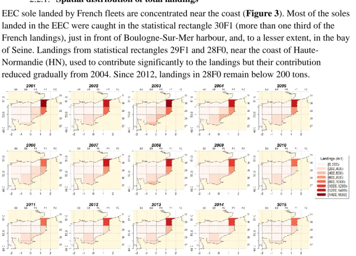
EEC sole landed by French fleets are concentrated near the coast (Figure 3). Most of the soles landed in the EEC were caught in the statistical rectangle 30F1 (more than one third of the French landings), just in front of Boulogne-Sur-Mer harbour, and, to a lesser extent, in the bay of Seine. Landings from statistical rectangles 29F1 and 28F0, near the coast of
Haute-Normandie (HN), used to contribute significantly to the landings but their contribution reduced gradually from 2004. Since 2012, landings in 28F0 remain below 200 tons.
Figure 3: French landings (in t) of Common Sole in EC by statistics rectangle between 2001 and 2015.
Regional landings 2.2.2.
In these three regions, Haut-de-France (HF), Haute-Normandie (HN) and Basse-Normandie (BN), sole landings have been decreasing since 2002/2003 (Figure 4). This decrease is particularly important in HN (reduction of 68% in 2015 compared to the maximum observed landings). The French quota increased in volume (not in proportion) between 2000 and 2008, it decreased until 2010 and dropped between 2013 and 2015 after a peak in 2013.
Figure 4: French landings of common sole in the EEC and quota (before the exchanges between EU countries) between 2000 and 2015
6
Spatial distribution of landings by fishing gear 2.2.3.
In the EEC, the French sole fishery is dominated by trammel nets which landed 65% of the sole landings in 2015. Then, bottom otter trawls contributed 21% of landings and fishing dredges and beam trawl to 9% and 3% respectively (Figure 5).
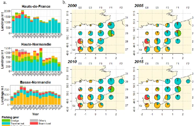
However, the contribution to the landings by gear varies greatly according to regions and geographical areas (Figure 6, a.). In HF, trammel netters are responsible for the majority of the landings (Figure 6, a.) while a very small proportion of the landings is made by trawlers (Figure 6, a.). In HN, from the early 2000s, the landings of trawlers (Otter Bottom Trawlers and Beam Trawlers) and trammel netters have gradually decreased whereas the volumes landed by dredgers remains (Figure 6, a.). Globally landings in HN have decreased more significantly than others regions (from nearly half of the observed landings in 2002 to less than 25% in 2015). In BN, except in 2000, the landings of bottom otter trawlers are always higher than trammels landings (Figure 6, a.). Overall, landings are subject to inter-annual variations following similar patterns in all regions. These landings peaked in 2002-2004 and are decreasing since.
Spatial landing distribution shows a decrease of trammel netters contribution in the Southwest (SW) of the EEC in favour of trawlers between 2000 and 2015 (Figure 6, b.). On the contrary, trammel netters contribution increased in the Northeast (NE). Fishing gear distribution is intermediate in the middle of the EEC (Figure 6, b.). Finally, local fishing practices stand out, particularly in two statistical rectangles, in the South-East with a high contribution of beam trawls and in the statistical rectangles 29F1 with an important contribution of dredge (Figure 6, b.). This spatial variability of the fishing gear is partly due to the inter-regional variability (Figure 6, a.) but there is also an important intra-regional variability (Appendix II).
In terms of regional distribution, two specific areas can be identified: one in the North (30F0 and 30F1) where only vessels from the HF area are operating and another in the South (28E8, 28E9, 27E9), only visited by the BN fishery. Other statistical rectangles cannot be allocated to a region because they are shared among regions. Landings in HN come from statistical rectangles shared with BN to the south and HF to the north (Appendix II).
Spatial and regional structuration of sole fisheries in the EEC is characterized by i) a fishing fleet in the NE dominated by netters from HF, ii) trawlers in the SW coming from BN and iii) an intermediate area in the middle of the EEC mixing trawlers and netters.
Figure 5: Contribution of the different gears to the French common sole landings in the EEC in 2015
7
Figure 6: a) Landings by region and by fishing gear from 2000 to 2015, b) spatial landings distribution by fishing gear. Pies are proportional to the volume landed in the statistical rectangles.
Spatial distribution of landings by mesh size used in the trammel net 2.2.4.
fishery
Trammel net is the main gear used by the French fleets to catch sole (65% of the French landings in 2015), whereas bottom trawls or dredges in the EEC will mostly use a unique mesh size range to target sole. Trammel netters used mainly 2 mesh size ranges to catch common soles in the EEC (Figure 7): (1) 90-99mm - 82%; (2) 100-119mm - 12%.
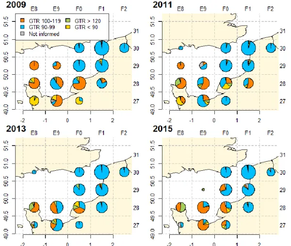
In the NE of the EEC, landings of trammel netters are dominated by 90-99mm mesh size range over the whole studied period. On the other hand, in the SW, landings of trammel netters are dominated by 100-119mm mesh size in 2015 whereas the share of mesh size 90-99mm were more important in 2011 and 2013 (Figure 8). In the middle of the EEC, the situation is intermediate: Before 2010, there were 3 mesh sizes used, “< 90”, “90-99” and “100-119”. Since 2010, the main mesh size has mostly been 100-119m and 90-99mm.
Figure 7: Contribution of the different mesh size range for the trammel net to the French common sole landings in the EEC in 2015.
8
Finally, local fishing practices stand out, particularly in the statistical rectangles 28E8, with an important contribution of bigger mesh size range (>120mm).
Figure 8: Mesh size range proportion in common sole landing in Eastern Channel for 2009, 2011, 2013 and 2015 from the SACROIS database.
Spatial distribution of landings by commercial category 2.2.5.
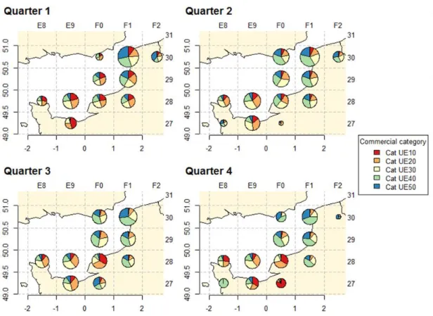
In 2015, common sole commercial categories (CC) are highly variable depending on the season and the area (Figure 9, please refer to table 1 for CC definitions). Sole landed are globally bigger in the 1st quarter and smaller in the 3rd quarter in all the EEC. Moreover, for each quarter, the weight of landed soles increases gradually from the north of the EEC to the south. In the north of the ECC under the latitude 50°, the weight of landed soles is particularly low.
Studying CC for trammel netters only shows again a gap between structure of CC between the NE of the EEC and the SW (Figure 10). Sole caught in in the North of the EEC are bigger than in the south with the limit at latitude 50°. Soles landed are particularly small in the NE in the 3rd and the 4th quarter and the CC shift toward small length over the years. The soles weight caught in the 1st quarter in SW is particularly important and decrease slightly until the 3rd quarter.
9
Figure 9: Common sole total landing in the EEC by statistical rectangle and by commercial category. Pies are proportional to the volume landed in each quarter in the given statistical rectangles.
Figure 10: Common sole total landing of the trammel netters in the EEC by statistical rectangle and by commercial category. Pies are proportional to the volume landed in each quarter in the given statistical rectangles.
10
2.3. Discussion
Most of soles landed were caught in the NE of the EEC and in the SW, and globally close to the coast. In the NE, the important landings close to the coast could be due to the trammel netters which are small vessels that cannot travel away from the coast. This could be linked with the spatial distribution of adult sole in the EEC and notably, the increase of concentration of adults common sole which come in coastal zones (Carpentier et al., 2009) during the spawning period. In addition, the results show that the SW of the EEC is mainly exploited by the BN fleets while the NE is exclusively exploited by the HN fleet. The intermediary area exploited by HN fleets but also partly by BN and HN fleets.
The great decrease of landing since 2004 cannot be imputed to quotas given that they were not a limiting factor until 2014 (with two exceptions in 2009 and 2010) (ICES, 2016). Several hypotheses may be proposed to explain this decrease: (1) Spatial distribution of the population changed since the early 2000s, (2) A decrease of biomass of common sole in the EEC, (3) the decrease of prices of common soles due to market fluctuations (in particular in North of France) coupled with a decrease of catches could speed a decrease of fishing effort up and, thus a decrease of landings. This last hypothesis is partly checked by the ICES common soles assessment (ICES, 2016). Indeed, peak of spawning biomass (Figure 2, b.) matched with peak of landings and the peak of recruitment at age 1 (Figure 2, c.) was followed by increased landing. For instance in 2002, the peak of recruitment at age 1 was followed by increased landing in HF and in BN, in 2003 and 2004 (Figure 6, a.).
This decrease of landings is found for each region exploiting common sole in the EEC. Note however an unexplained peak of landings in HN in 2009, it could be a data acquisition error because, in 2009, the data acquisition procedure and the database of logbook changed.
The method to affect regions at each landing can imply a bias because landings are affected at the landing regions based on landing harbour and not at the home port regions. So regions are not strictly representatives of regional fishing’s practices. However, for trammel netters, landing port is usually the fishing home port because they are small vessels fishing close to the coast.
Trammel netters used mainly 2 mesh size ranges of the inner panel to catch common sole in the EEC: 90-99mm and 100-119mm with a spatial structuration. In the NE, since 2009, netters used only the 90-99mm range and in the SW in 2015 netters used mainly the 100-119mm range. The use of the 100-100-119mm range was expanded in 2014 and 2015 mainly to increase the length structure of the catch to improve the valorisation of the landings. That increase was partly induced by the OPBN (a producer’s organisations in BN) that encouraged fishermen to improve the selectivity by increasing the minimum size of landing from 24cm (the official minimum landing size) to 26cm.
Finally, for the global landings and for the trammel netter, the individual weight of common soles landed in the NE in the EEC is lower than in the SW with a limit in the latitude 50°. This suggests that the length structure of the catches varies depending on the fishing area or/and the fishing practise given the spatial structuration in terms of fishing gear and mesh size ranges. In addition, the decrease of sole weight in the second semester could, partly, due to recruitment (small fish entering the stock) in the 3rd quarter which brings out a higher
11
proportion of sole caught coupled with the adult dispersal after the spawning period. In the following part, this hypothesis was tested for the trammels netters.
3. Length structure of common sole captures by trammel nets in
the EEC
3.1. Introduction
In the previous section, commercial categories of soles landed in the EEC show a high spatial variability with soles landed in the north of the EEC smaller than in the south. In parallel, fishing practises in terms of fishing gears and mesh sizes used by trammel netters show spatial structuration in the EEC with, notably, a majority of 90-99mm mesh size range used by trammels netters in the North and a majority of 100-119mm mesh size range in the South. This suggests a link between the fishing gear selectivity and the variability in the length distribution. Fishing gear selectivity was analysed from fishing gear mesh size which is the main (but not the only) parameter influencing the selectivity. Few authors showed that the fish size selectivity of trammel nets depends primarily on the mesh size of inner net (Figure 11) (Erzini et al., 2006, Kitahara, 1968; Losanes et al., 1992b; Purbayanto et al., 2000; Salvanes, 1991).
Figure 11: Selectivity curves for Solea solea in Basque country using SELECT models; dashed line: 90mm inner panel mesh, continuous line: 100mm inner panel mesh, bold line: 110mm inner panel mesh (Erzini et al., 2006).
However, the length distribution in catch is also directly linked to the length distribution of the underlying population. It is then important to take into account the structure of the population and test the hypothesis of the existence of 3 isolated sub-populations in the EEC (potential variation in population structure, in growth, in length and age at maturity…). In addition, changes in the population structure over the years due to recruitment fluctuations could also influence the catch-at-length.
In this section, we will focus on the length structure of the catches to assess the impact of (i) nets selectivity, (ii) length structure of population and (iii) the interaction of these two parameters from catch-at-length data of a fraction of commercial catches.
12
3.2. Materials & Methods
Data 3.2.1.
OBSMER
The OSMER program aims at observing, in situ, French fishing activities and their catches. During a trip, for a fraction of fishing operations, the observer identifies the species caught; records the weight by species and catch category (landings/discards), and measures all individuals from commercial species. For each commercial species, the number per length (1 cm group) and per haul is recorded. The commercial fishery database OBSMER was used for the length data analysis of the catches from 2009-2015 in the EEC. The haul by haul data from trammel netter includes the fishing date, the exact fishing position (latitude and longitude), the statistical rectangle, the fishing gear category, the home port of the fishing vessel, the catch category (landings or discard) and the catch in numbers at length. As for SACROIS, the mesh sizes between 40 and 50mm were doubled for the trammel net.
Nurseries
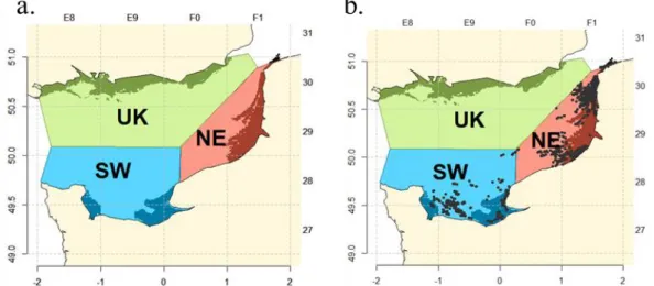
The nurseries area is an essential habitat for juvenile stages of common sole. Therefore, fishing operation made in nursery area were identified using Age 1 sole distribution as identified by Rochette et al., 2010 (Figure 12, a).
Subareas
The hypothesis of low connectivity between 3 sub-populations, described in the introduction, can potentially affect the length structure of catches. The 3 subareas UK, Southwest (SW) and Northeast (NE), consistent with the suggested existence of 3 isolated subs-population in the EEC (Rochette et al., 2012) were introduced in this study (Figure 12, a).
Figure 12: a) 3 subareas colored in blue, red, and green and the darker areas along the coast representing the nurseries area; b) Position of trammel net hauls with common sole in the EEC from Obsmer between 2009 and 2015
Analytical Methods 3.2.2.
Mean length Cartography
In each statistical rectangle, the mean length is computed by statistical rectangle and by mesh sizes range (with more than 50 individuals gathered).
13
This first descriptive method allows for a visual description of the spatial distribution of mean length of sole catches in the EEC.
Statistical analyses
In order to assess the spatio-temporal variability of catches length structure and the impact of fishing practises, 5 variables were selected (Table 2).
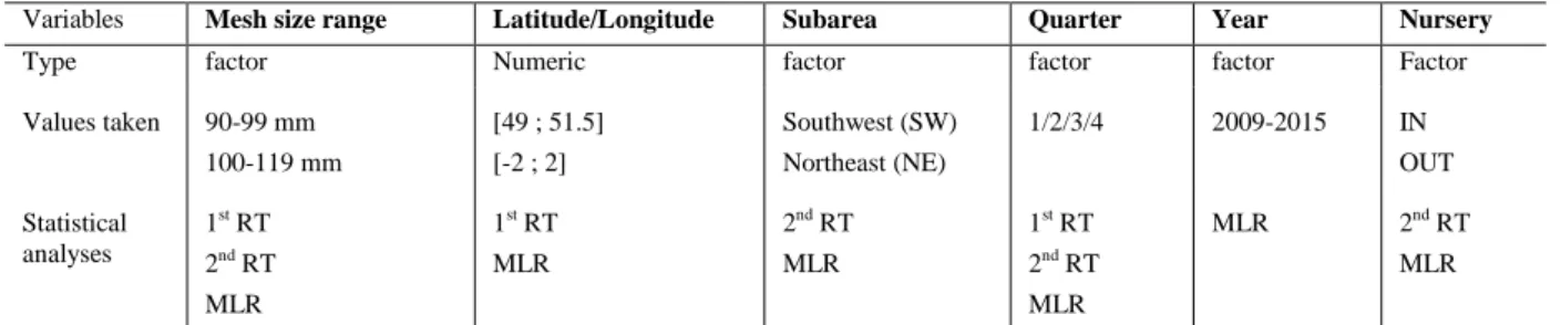
Table 2: Description of variables used in the statistical analyses: 2 regression trees (RT) and 1 multinomial logistic regression (MLR)
Variables Mesh size range Latitude/Longitude Subarea Quarter Year Nursery
Type factor Numeric factor factor factor Factor
Values taken 90-99 mm 100-119 mm [49 ; 51.5] [-2 ; 2] Southwest (SW) Northeast (NE) 1/2/3/4 2009-2015 IN OUT Statistical analyses 1st RT 2nd RT MLR 1st RT MLR 2nd RT MLR 1st RT 2nd RT MLR MLR 2nd RT MLR
In the analysis the mesh sizes were restricted to two main mesh size ranges used (90-99mm and 100-119mm) as they were responsible for most of the landings (87%) during the period 2000-2014 (94% in 2015).
Spatial features of the landings length structure were explored using either haul by haul latitudinal or longitudinal information provided by Obsmer data (c.f. section 3.2.2), or the 3 subareas defined in (Figure 12, b). Data for the UK subarea are hardly available because French netters do not fish in these grounds, so the UK subarea was removed from this analysis. The OBSMER geolocation allows to locate each haul station inside or outside nurseries grounds in order to create an IN/OUT variable. Location of nursery grounds is defined in section 3.2.1.
Regression tree
Spatio-temporal variability of mean length was first assessed using regression trees. This method allows to class variables affecting the mean length of captures according to mean length variability given their importance during the classification. Interaction effects were also suggested thanks to the partitioning construction of the trees. The analysis by mean length approach requires an aggregation of the individual fish information contained in OBSMER (the two levels of aggregation tested are presented later in this section) but provides an initial understanding on the determinants of the mean length of the captures. The Regression tree approach based on CART (Classification and Regression trees) uses recursive partitioning to determine a series of binary rules that divide the data into smaller more homogeneous subgroups. The splitting criterion, which is used to decide which variable gives the best split is: 𝑆𝑆𝑇− (𝑆𝑆𝐿 + 𝑆𝑆𝑅) where 𝑆𝑆𝑇 = ∑(𝑦𝑖 − 𝑦̅) ² is the sum of squares for the node, and 𝑆𝑆𝐿 and 𝑆𝑆𝑅 are the sums of squares for the right and left son, respectively. The aim is to maximize the between group sum of squares.
First of all, the best level of simplification is determined thanks to the “complexity parameter” setting a complexity threshold (default value 0.01). Then, pruning, i.e. the level of simplification of the tree, is validated or tightened using cross validation in checking the number of splits from which the cross validation error increases. Finally, pruning has been
14
further improved by taking into account the error bars (1-SE rule). Residuals were also checked to compare observed mean lengths and predicted values.
The CART algorithm uses a surrogate split process to overcome the missing data. It can classify, a posteriori, an individual with no modality for a constitutive variable of the tree. Moreover a regression tree constructed with the CART algorithm can work with all types of variables: qualitative, ordinal and continuous quantitative (Santos, 2015).
Observed haul level data were aggregated into combinations of factors. Two different groups of factors are studied separately, by changing only the spatial variable:
- 1st group: Latitude, Longitude, Mesh size range, Quarter, Nurseries, Year
- 2nd group : Subarea, Mesh size range, Quarter, Nurseries, Year
For the 2 regressions, only combinations with more than 20 individuals were kept (1st group: 85% of individuals, 2nd group: 83%) using the following explanatory variables:
- 1st group: Latitude, Longitude, Mesh size range, Quarter, Nurseries
- 2nd group : Subarea, Mesh size range, Quarter, Nurseries
Therefore, the statistical individual is the average individual for each variable combination (including year) with more than 20 individuals. The year effect was not used in the analysis but used to realise cross-validation RT By not including the "year" effect in the RT it was possible to get a variable combination for each year (7 between 2009 and 52015) that were used to perform cross-validation.
To pool individual data into latitude and longitude, these two variables were aggregated in small group of 1/8° for latitude and 1/4° for longitude. Latitude and longitude were then considered as numeric variables in the regression procedure.
Multinomial logistic regression
A Multinomial logistic regression aims to model the probability of a given sole to belong to a length class. Therefore, it allows exploring length distribution variability.
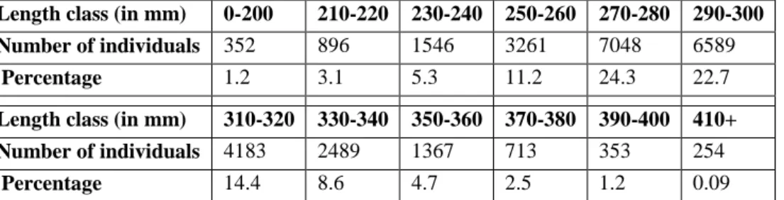
Individual total lengths were aggregated into 12 length classes (Table 3). The first and last percentiles of the sole length distribution were aggregated into two length classes between 0mm and 200mm (0-200), and 410mm and 490mm (410+), respectively. In between 210mm and 400mm, lengths were aggregated by 20 mm length class. This discretization of the length structure allows the thorough description of the largest share of the distribution without increasing too much the number of classes.
Table 3: Length classes used for the multinomial logistic regression with the number of individuals in each class and the corresponding percentage.
Length class (in mm) 0-200 210-220 230-240 250-260 270-280 290-300
Number of individuals 352 896 1546 3261 7048 6589
Percentage 1.2 3.1 5.3 11.2 24.3 22.7
Length class (in mm) 310-320 330-340 350-360 370-380 390-400 410+
Number of individuals 4183 2489 1367 713 353 254
Percentage 14.4 8.6 4.7 2.5 1.2 0.09
The probability that a sole 𝝎 belongs to a length class 𝒚𝒌 (k=12) was defined as
15
where Y was the dependant variable and X were the exploratory variables with the constraint ∑ 𝝅𝒌(𝝎)
𝒌
= 𝟏 Therefore the likelihood is given by
𝑳 = ∏[𝝅𝟏(𝝎)]𝒚𝟏(𝝎)× … × [𝝅 𝑲(𝝎)]𝒚𝑲(𝝎) 𝒌 ( 2 ) Where 𝒚𝒌(𝝎) = { 𝟏 𝒊𝒇 𝒀(𝝎) = 𝒚𝒌 𝟎 𝒐𝒕𝒉𝒆𝒓𝒘𝒊𝒔𝒆
The principle of the multinomial logistic regression is to model K-1 (here 12-1) ratio of probability (𝝅𝒌). One category (length class) is set as the base line. In our case the reference
category was defined as the first length class [0; 200]. Logit for 𝒚𝒌 is then computed as:
𝑪𝒌 = 𝒍𝒏 𝝅𝒌
𝝅𝟎−𝟐𝟑𝟎= 𝒂𝟎,𝒌+ 𝒂𝟏,𝒌𝑿𝟏+ ⋯ + 𝒂𝑱,𝒌𝑿𝑱
( 3 )
And, therefore, probabilities at posteriori are 𝝅𝒌=
𝒆𝑪𝒌
𝟏 + ∑𝑲−𝟏𝒆𝑪𝒌 𝒌=𝟏
( 4 )
Finally, the log-likelihood was maximized
𝑳𝑳 = ∑ 𝒚𝟏(𝝎) 𝐥𝐧 𝝅𝟏(𝝎) + ⋯ + 𝒚𝑲(𝝎) 𝐥𝐧 𝝅𝑲(𝝎)
𝒌
( 5 )
Multinomial regression was implemented in R (R Core Team , 2014) using the package ‘nnet’ and the ‘multinom’ function (Ripley and Venables, 2016). Multinomial model were fitted using neural networks allowing the definition of a large number of parameters and length classes.
The model selection was selected through minimization of the Akaike’s Information Criterion (AIC). The fitting quality of the regression was assessed via the McFadden Pseudo-R² and the global significance was assessed with a likelihood-ratio test comparing the selected model and the null model. Then, prediction quality was evaluated by comparing the residuals of the observed and predicted length distribution of all combination of variables kept in the model. To compare predicted distribution and observed distribution for a particular variable, the mean of the predicted length distribution for this variable was computed. In addition, the dataset from Obsmer was segregated into two groups: (1) a learning sample, and (2) a validation sample to perform a cross-validation. The validation sample was selected extracting randomly 10% of each combination of the 5 variables (Subarea, Mesh size range, Quarter, Year, and Nursery). The reclassification quality of the data of the validation sample was studied using a Model build from the learning sample.
16
3.3. Results
Mean length variability 3.3.1.
Mean length Cartography
Only a few statistical rectangles are fished with 100-119 mm mesh size trammel nets. Therefore only the mean lengths for all trammels nets (all mesh sizes merged, subsequently named “all trammels”) and for 90-99 mm mesh size trammels (subsequently named “90_99 trammels) are shown. The mean lengths of the “all trammels” show a gradient with bigger average sizes in the south of the EEC and smaller ones in the north (Figure 13). These differences could be explained by differences in the mesh sizes used in the different regions but this gradient is also found for the “90-99 trammels” meaning that differences are therefore not only due to mesh size. These differences can be found each year since 2009 (Appendix III).
Figure 13: Mean length by statistical rectangles of catches between 2009 and 2015: a) for all mesh size range, b) only for 90-99mm mesh size range
Throughout the year, the mean lengths show a gradient with an increase from the NE to the SW, (Figure 14, a). In the South of EEC, for all mesh sizes, there is a peak in the mean length of catches during the 2nd and 3rd quarter. In the North of EC, the mean lengths gradually decrease between the 1st and 4th quarter. A similar gradient can be observed for catches with the 90-99 mm mesh size range (Figure 14, b). Moreover, for this mesh size range, mean lengths are bigger the first two quarters of the year.
Figure 14: Mean length by statistical rectangle and by quarter of catches between 2009 and 2015: a) for all mesh size range, b) only for 90-99mm mesh size range
17
Regression tree
The 1st RT was pruned keeping 7 splits (Figure 15). The quality of the residuals is correct with 90% of them below 20 mm and 59% of residuals below 10 mm (Appendix III). In the 1st RT, the mesh size range is the variable that has the most impact on the means. The quarter effect then stands out for both mesh size ranges (100-119 mm and 90-99 mm). Overall, the soles caught in the 2nd quarter are, on average, larger than in the 3rd quarter. We can notice that the quarter effect for 90-99 mm mesh size is consistent with the observations made previously (Figure 14, b). In the 90-99 mm mesh size branch, two areas are identified in terms of longitude. There is a lag of 0.45° between the two different longitudinal limits highlighted (0.75°E in the two first quarters and 1.2°E in the two last quarters) in the first RT depending on the time of the year, but in both cases soles are on average smaller East of the EEC. Finally, fishing on nursery areas affects mean lengths with bigger soles caught out of the nursery grounds.
Figure 15: a) Regression tree developed from mesh size, quarter, nursery, and latitude and longitude. Choosing cuts are indicated on each branch in italics. The mean lengths and the numbers of individuals (combination in our case) are indicated in bold at each leaf at the base of the tree. b) Map of the Eastern Channel, where points represent trammel net hauls for both mesh size ranges and lines represent longitudes highlighted in the 1st regression tree.
The 2nd RT was pruned keeping 6 splits (Figure 16). The quality of the residuals is correct with 94% of residuals below 20 mm and 62% below 10 mm (Appendix IV). This RT shows the same effects, the subarea is highlighted as a significant variable. The soles caught in the NE of the EEC are smaller than those in the SW and in the UK subarea. However, this difference in the mean lengths is tenuous.
Differences in the variables affecting mean lengths depending on the mesh size ranges suggest the existence of interactions between variables. Indeed, without interaction, variables would affect mean lengths in the same proportion whatever the mesh size used. Therefore, 3 interactions could exist between: Mesh size and Quarter, Mesh size and Nursery and Mesh size and Subarea.
18
Figure 16: Regression tree developed from mesh size, quarter, nursery and subarea. Choosing splits are indicated on each branch in italics. The mean lengths and the numbers of individuals (combination in our case) are indicated in bold at each leaf at the base of the tree.
Length class distribution 3.3.1.
The model selection procedure using the AIC criterion led to select a complete model with 5 variables and 7 interactions:
Single effect: mesh size range, year, quarter, nursery and subarea
Interaction effect: mesh size x subarea, mesh size x nursery, subarea x nursery, subarea x
quarter, nursery x year, nursery x quarter and mesh size x quarter
The McFadden Pseudo-R² is fairly low: 0.062. However, the likelihood-ratio test is clearly significant (p<2.2.10-16). Residuals (Figure 17) show a globally homogeneous distribution but the residuals structure is quite peculiar with a global underprediction for the smallest and the biggest length classes and an overprediction for the average length class. The model tends to underpredict the probability of belonging to the length classes 240-250, 320-330 and 340-350 and to underpredict the probability of belonging to length classes 270-280 and 290-300. Moreover for the last two length class, the residuals variability is higher. Finally, the analysis of variance indicates (Appendix V) that all variables and interactions kept in the model contribute significantly to explain the model variability. The cross validation shows that the model predicts only 4 length classes between 270mm and 340mm (Appendix VI, a.). It is coherent results given these are the main length classes. And from either side of these predicted length classes, the observed length classes are homogeneously distributed (Appendix VI, b.).
19
In the following section, the means of predicted probabilities of belonging to each length class for each explanatory variable were plotted against length distributions of capture in order to judge the predictive quality of the Model.
Fishing gear
The observed length distribution (Figure 18) shows a shift toward the biggest length class for the captures with a mesh size in the 100-119mm range compared to the 90-99 range. The shape of the distribution of the 90-99mm mesh size range is narrower than 100-119mm one. The multinomial regression model confirms a mesh size effect on the length distribution of the catch (Appendix V). The superposition of predicted values and observed values shows a mismatch (Figure 18). The mismatch is particularly important for the 100-119 mesh size range with overprediction on the small length and underprediction on the large length. However, the predicted distributions follow the main distribution patterns: (1) the distribution shift between the two mesh size ranges is predicted but slightly underestimated; (2) The difference in shape of the two respective distributions is well predicted.
Figure 18: Predicted and observed length distributions of capture of common sole for two mesh size ranges 100-119mm and 90-99mm
Subarea
Observed length distributions show a great shift depending on the 2 subareas with a maximum around the length class 290-300 mm (Figure 19, a.). The shape of the distribution in the NE of the EEC is narrower than in the SW. In SW, frequencies of captures of small soles (smaller than 260mm) are very low and much lower than in NE. Furthermore, frequencies of captures of large soles (bigger than 300mm) are much higher.
Doing the analysis with the 2 mesh size ranges leads to the same observation (Figure 19, b.
and c.). The shape of the distribution in the NE of the EEC is narrower than in the SW. With
the 100-119mm mesh size range, the distributions show difference in mode and in shape (Figure 19, c.). In the SW, the distribution is wider than in the NE.
The multinomial regression model confirms a subarea effect on the length distribution of the catch and an interaction effect between the subarea and the mesh size range (Appendix V). But the model tends to underpredict the difference between the two subareas as shown the predicted probabilities (Figure 19, a.). On the large length, the length frequencies are overpredicted in the NE and underpredicted in the SW. In addition, the predicted frequencies are not very well predicted for the 100-119mm mesh size range, while the predicted frequencies are well predicted for the 90-99mm mesh size range.
20
Figure 19: Predicted and observed length distribution of capture of common sole for the two subareas Northeast and Southwest (respectively in blue and in orange) for a) global catch, b) catches with mesh size in the range 90-99mm, and c) catches with mesh size in the range 100-119mm
Nurseries
A global view of length distributions in the nursery (Figure 20, a.) show a tenuous difference in catch at length between soles caught in and out nursery areas, except a slight shift toward the biggest length class outside the nursery area. However, length distribution of captures in and out of the nursery areas is very different depending on the mesh size range used (Figure
20, b. and c.); there is no significant difference in the distributions associated with the mesh
size range 90-99m, whereas the difference (a shift and a difference in shape) is particularly important in the case of the range 100-119mm (Figure 20, c.).
The multinomial regression model confirms a nursery effect on the length distribution of the catch and an interaction effect between the nursery and the mesh size range (Appendix V). But the model tends to underpredict the length frequencies of captures of small soles and to overpredict the length frequencies of captures of large soles (Figure 20, a.).
Figure 20: Predicted and observed length distributions of capture of common sole in or out the nursery areas (respectively in red and in green) for a) global catch, b) catches with mesh size range 90-99mm, and c) catches with mesh size range 100-119m
The multinomial regression model indicates that the interaction effect between the quarter and the nursery is significant (Appendix V). This is particularly interesting to take into account this interaction given the seasonal spawning migration.
With the mesh size range 90-99mm (Figure 21, a.), length distributions of soles caught outside and inside the nursery areas vary throughout the year. The proportion of small soles