HYDROTEL 1.0: user's guide.

(1)

Author Role:

Title, Monographic:

HYDROTEL 1.0 : user's Guide

Translated Title:

Reprint Status:

Edition:

Author, Subsidiary:

Author Role:

Place of Publication:

Québec

Publisher Name:

INRS-Eau

Date of Publication:

1988

Original Publication Date:

7 juillet 1988

Volume Identification:

Extent of Work:

vi, 76

Packaging Method:

pages

Series Editor:

Series Editor Role:

Series Title:

INRS-Eau, Rapport de recherche

Series Volume ID: 260

Location/URL:

ISBN:

2-89146-257-2

Notes:

Rapport annuel 1988-1989

Abstract:

Rapport rédigé pour Canada Center for Remote Sensing, Application Division &

Canada Environment, Hydrology division

15.00$

Call Number:

R000260

Keywords:

rapport/ ok/ dl

(2)

USER'S

GUIDE

by Jean-Pierre FORTIN Jean-Pierre VILLENEUVE Claude BLANCHETTE Denis ISABEL Hilaire PROULX

Scientific Report INRS-Eau No 260

By: Université du Québec Institut national de la recherche scientifique INRS-Eau 2700, rue Einstein C.P.7500 SAINTE-FOY, (Québec) G1 V 4C7 CANADA 7 July 1988

For: Application Division

Canada Center for Remote Sensing 1547 Marivale Road OTTAWA, (Ontario) K1AOY7 and Hydrology Division Environment Canada OTTAWA, (Ontario) K1AOE7

(3)

TABLE OF CONTENTS . . . . LIST OF TABLES . . . . LIST OF FIGURES . . . . PART 1 1.1 1.2 1.3 1.4 PART 2 2.1 2.2 2.2.1 2.2.2 2.2.3 2.3 2.3.1 2.3.2 2.3.3 2.3.3.1 2.3.3.2 2.3.3.3 2.3.4 2.3.5 2.3.5.1 2.3.5.1.1 2.3.5.1.2 2.3.5.1.3 2.3.5.2 2.3.5.2.1 2.3.5.3 2.3.5.3.1 2.3.5.4 2.3.5.4.1 2.3.5.4.1.1 2.3.5.4.1.2 2.3.5.4.1.3 2.3.5.4.1.4 2.3.5.4.1.5 2.3.5.5 2.3.5.5.1 2.3.5.6 GENERAL INFORMATION . . . . SOFTWARE MAIN CHARACTERISTICS AND HARDWARE REQUIREMENTS .. INTRODUCTION . . . . ORGANIZATION OF THE MANUAL . . . . SOFTWARE AVAILABILITY AND INFORMATION ... . THE HYDROTEL PROGRAM (1. 0) . . . . GENERAL MODEL STRUCTURE . . . . GETTING STARTED . . . . List of files on diskettes . . . .

Installing HYDROTEL 1. 0 . . . .

Test data and structure of data files ... . US ING HYDROTEL (1. 0) . . . . Starting HYDROTEL 1.0 . . . . Main menu . . . .

Sub-menu #1.0: input of simulation parameters ... .

Sub-menu #1.1: paths of files ... .

Sub-menu#1.2: temporal parameters ... .

Sub-menu #1.3: spatial parameters ... .

Sub-menu #2.0: input of physiography data files ... .

Sub-menu #3.0: sub-models . . . .

Sub-menu #3.1: interpolation of precipitation ... .

Sub-menu #3.1.1: Thiessen polygons ... .

Sub-menu #3.1.2: weighted mean of nearest three stations

Sub-menu #3.1.3: arithmetic mean of nearest three

stations . . . .

Sub-menu #3.2: snowmel t . . . .

Sub-menu #3.2.1: modified degree-day method ... .

Sub-men~ #3.3: evapotranspiration ... .

Sub-menu #3.3.1: input data for Thorthwaite PE ... .

Sub-menu #3.4: vertical water budget ... .

Sub-menu #3.4.1: input data for CEQUEAU ... .

Sub-menu #3.4.1.1: runoff on impervious areas ... .

Sub-menu #3.4.1.2: unsaturated zone reservoir ... .

Sub-menu #3.4.1.3: saturated zone reservoir ... .

Sub-menu #3.4.1.4: lakes and marshes ... .

Sub-menu #3.4.1.5: initial levels in reservoirs ... .

Sub-menu #3.5: surface and sub-surface runoff ... .

Sub-menu #3.5.1: kinematic wave equations ... .

Sub-menu #3.6: channel routing ... .

i 1 2 2 4 4 6 7 8 8 9 10 14 14 15 15 16 17 19 20 22 23 24 25 25 25 26 27 28 29 30 31 32 33 34 35 36 37 38 39

(4)

2.3.6 2.3.6.1 2.3.6.2 2.3.6.3 2.4 2.4.1 2.4.1.1 2.4.1.2 2.4.1.3 2.4.2 2.4.2.1 2.4.2.2 2.4.2.2.1 2.4.2.2.2 2.5 PART 3 3.1 3.2 3.2.1 3.2.2 3.2.3 3.3 3.3.1 3.3.2 3.3.3 3.4 3.4.1 3.4.1.1 3.4.1.2 3.5 3.5.1 3.5.1.1 3.5.1.2 3.6 3.6.1 3.6.2

Sub-menu #4.0: output options ... .

Sub-menu #4.1: watch ... .

Sub-menu #4.2: display ... .

Sub-menu t14. 3 : save

CALIBRATION OF MODEL PARAMETERS AND INITIALIZATION OF STATE VARIABLES ... . Calibration of model parameters ... . Control criteria ... . Pre-calibration sensitivity analysis ... . Subjective calibration ... . Initialization of state variables ... . Vertical water profile ... . Water in transit ... . First simulation on a new basin ... . AlI further simulations on a basin for which

41 41 44 46 48 48 48 49 49 49 50 51 51

initialization files do exist ... 54

INTEGRATION OF USER'S DEVELOPED SUB-MODELS ... . MAIN SIMULATION EQUATIONS AND FLOW CHARTS ... . INTRODUCTION ... . SPATIAL DISTRIBUTION OF PRECIPITATION ... . Thiessen po1ygons ... . Weighted mean of nearest three stations ... . Arithmetic mean of nearest three stations ... . SNOW COVER SIMULATION AND MELTING ... . Transformation of rainfa11 into snowfa11 ... . Simulation of snowpack transformation and me1t ... . Input variables ... . EVAPOTRANSPIRATION ... . Thorthwaite potential evapotranspiration ... . The equa tion ... ; ... . Input data .. ' ... . VERTICAL WATER BUDGET ... . CEQUEAU (modified) ... . Description of the function ... . Input data .•... SURFACE AND SUB-SURFACE RUNOFF ... . Kinematic wave equations ... . Input data ... . i i 54 55 56 56 56 57 57 57 57 58 59 60 60 60 61 62 62 62 64 66 67 68

(5)

3.7.2 3.8 REFERENCES Input data ... . LAND-USE CLASSIFICATION ....•...•..••••••••••••...•.. i i i 71 72 74

(6)

Table 2.1 Table 3.1

Julian days ... . 18

Values of Manning's roughness coefficient n for flow over squares, as a function of land-use classes.

(7)

Figure 1.1 Figure 2.1 Figure 2.2 Figure 2.3 Figure 2.4 Figure 2.5 Figure 2.6 Figure 2.7 Figure 2.8 Figure 2.9

Integrated analysis of physical, remotely sensed and meteorological data for steamflow simulation and

forecasting by PHYSlTEL, IMATEL and HYDROTEL ... .

3

Spatial structure of the model ... 7

Streamflow and climatological stations on the Eaton basin 10 Main menu ... 15

Sub-menu #1.0: input of simulation parameters .. , ... 16

Sub-menu tH.1: paths to files ... 16

Sub-menu #1.2: temporal parameters ... 19

Sub-menu #1.3: spatial parameters ... 20

Sub-menu #2.0: input of physiography data files ... 21

Monitoring of file input a) options 1 to 5 b) option 7 ... 21

Figure 2.10 Sub-menu #3.0: sub-models ... 22

Figure 2.11 Sub-menu #3.1: interpolation of precipitation ... 23

Figure 2.12 Sub-menu #3.1.1: Thiessen polygons ... 24

Figure 2.13 Sub-menu #3.1.2: weighted mean of nearest three stations 25 Figure 2.14 Sub-menu #3.1.3: arithmetic mean of nearest three stations 25 Figure 2.15 Sub-menu #3.2: snowmel t ... 26

Figure 2.16 Sub-menu #3.2.1: modified degree-day method ... 27

Figure 2.17 Sub-menu #3.3: evapotranspiration ... 28

Figure 2.18 Sub-menu #3.3.1: input data for Thorthwaite PE ... 29

Figure 2.19 Sub-menu #3.4: vertical water budget ... 30

Figure 2.20 Sub-menu #3.4.1: input data for CEQUEAU 31

Figure 2.21 Sub-menu #3.4.1.1: runoff on impervious areas 32

Figure 2.22 Sub-menu #3.4.1.2: unsaturated zone reservoir 33

(8)

Figure 2.24 Sub-menu #3.4.1.4: lakes and marshes 35

Figure 2.25 Sub-menu #3.4.1.5: initial levels in reservoirs ... 36

Figure 2.26 Sub-menu #3.5: surface and sub-surface runoff . ... 37

Figure 2.27 Sub-menu #3.5.1: kinematic wave equations ... 38

Figure 2.28 Sub-menu #3.6: channel routing ... 39

Figure 2.29 Sub-menu #3.6.1: modified kinematic wave equations ... 40

Figure 2.30 Sub-menu #4.0: output options ... 41

Figure 2.31 Sub-menu #4.1: watch... .... ... 41

Figure 2.32 Tabular informations on variables related to squares ... 42

Figure 2.33 Tabular informations on variables related to reaches ... 43

Figure 2.34 Tabular informations on variables related to vertical water budget ... 43

Figure 2.35 Sub-menu #4.2: display... 44

Figure 2.36 Streamflow hydrograph ... ... 45

Figure 2.37 Sub-menu #4.3: save.... . . 46

Figure 2.38 Main daily temperature ... 47

Figure 2.39 Available water from rain and/or melt ... 47

Figure 3.1 Vertical water budget adapted from the CEQUEAU model . .... 63

Figure 3.2 Surface and sub-surface runoff and channel flow ... 67

(9)

(10)

PART 1 GENERAL INFORMATION

1.1 SOFTWARE MAIN CHARACTERISTICS AND HARDWARE REQUIREMENTS

Name: HYDROTEL 1.0

Objective: Simulation of streamflows using ground and remotely

sensed data.

Programming languages: Mostly MS "C". The "precipitation module" is temporary

written in BASIC.

Type of microcomputer: IBM PC/XT or AT and compatibles.

Memory requirements: 640K.

Written by: Claude Blanchette, Denis Isabel, Jean-Pierre Fortin and

Hilaire Proulx.

1.2 INTRODUCTION

Considering, as others (Peck et al., 1981; Rango, 1985), that there was a need for the development of hydrological models compatible with remotely sensed

data, INRS-Eau began such a development a few years ago. Work was undertaken

on various aspects of hydrological modelling, namely: type of simulation for

surface and sub-surface runoff as weIl as for channel routing, determination of basin topography from a digital elevation model (DEM), display and analysis of images on microcomputers, land-use determination for hydrological purposes, integration of weather radar and station data ...

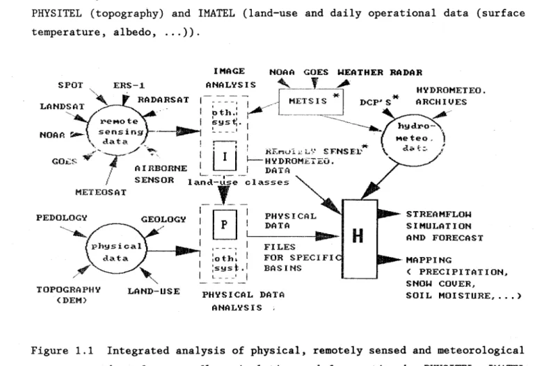
At the beginning, the model was seen as one program allowing determination of basin topography from DEM, land-use determination from the analysis of remotely

sensed images and hydrological simulation and forecasting. As seen in

figure 1.1, it was thought later on that the large number of tasks would be handled more easily by three interrelated software packages instead of one.

(11)

The HYDROTEL package will be devoted to hydrological simulation and

forecasting. As such, it will receive input data in the proper format from

PHYSITEL (topography) and IMATEL (land-use and daily operational data (surface temperature, albedo, ... )).

1 MAGE NOAA GOES WEATHER RADAR

SPOT,

.

ERS-l. ANALYSIS

[ J

~_, __

I __

~

HYDROHETEO.

"'~.

RADARSAT

I---=---=-:

l '

HETSIS.J(' DCP'S*

LAND~(H . .' . l ' ' : AJIa/

"'1

reMo,te.

L

__

----!

~:~ti·

i

---=~'----__...

NOM

~\,

S::::a.1ng/,

.-~

; ---;

~

'..

* .

)

-"'''''~T'/

":'-:

1

L!J"

.ti:E...,u'l", L',' SFNSE1: \ dcot.:,

.-GOL~ ~ ~HYDROME~EÜ.

1 AIIŒORNE 1 1 DATA

l ' .

-1 SENSOR land-use classes

METEOSAT

_J __

PEDOLOCY TOPOGRAPHY (DEH) GEOLOGY LAND-USE

r:l

1 PHYSICAL

~

:<--_D_A_T_A_--1 1 , ' ,oth. 1 ;Syst.1 L _ _ - ' 1 FILES BASINS PHYSICAL DATA ANALYSIS STREAMFLOW SIMULATION AND FORECAST ( PRECIPITATION. SNOW COVER, SOIL MOISTURE, . . . )

Figure 1.1 Integrated analysis of physical, remotely sensed and meteorological data for steamflow simulation and forecasting by PHYSITEL, IMATEL and HYDROTEL.

Writing of the HYDROTEL main program itself began only a few months ago. As

seen by INRS-Eau the status of the current HYDROTEL version is the following:

HYDROTEL 1.0 structure has been conceived and programmed to facilitate the graduaI addition of all wanted options to a fully "à la carte" model, as weIl as the input and output of G.I.S. and time dependent data;

HYDROTEL 1.0 is considered as a first working prototype, with a minimum of options and should be regarded as only a step in the development of the model originally conceived;

(12)

HYDROTEL 1.0 can already make use of topography and land-use information;

HYDROTEL 1.0 should not be compared to any fully developed model;

HYDROTEL 1.0 should be used mainly to get acquainted with the model and suggest what options should be added in the following versions.

INRS-Eau will try to make development versions (l.nn) available to those participating in the tests whenever the addition of new options well make it worthwhile.

1.3 ORGANIZATION OF THE MANDAL

Part "ONE" of the manual contents general information on HYDROTEL 1.0.

In part "TWO", the user is first told how to install the computer program.

Information on the data set furnished with the program is then given. This

data set is made available to the user to allow him to get acquainted with the

model. Information on how to start the program is next given. This is

followed by a detailed information, window by window, on the simulation choices, and input data.

A description of the main simulation methods available with HYDROTEL 1.00 is finally given in part "TRREE" , together with hints on how to select values for model parameters.

1.4 SOFTWARE AVAILABILITY AND INFORMATION

The current version (1.0) of HYDROTEL is available only to CCRS and Environment Canada personnel participating in the testing of that version, to help defining the options that should be available in HYDROTEL (2.nn).

(13)

For informations, contact:

Prof. Jean-Pierre Fortin INRS-Eau

C.P.

7500 Sainte-Foy (Québec) G1V 4C7 CANADA Telephone: (418) 654-2591 Telex: 051-31623 Fax: (418) 654-2615

(14)

(15)

PART 2 THE HYDROTEL PROGRAM (1. 0)

2.1 GENERAL MODEL STRUCTURE

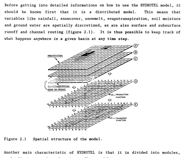
Before getting into detailed informations on how to use the HYDROTEL model, it

should be known first that it is a distributed model. This me ans that

variables like rainfall, snowcover, snowmelt, evapotranspiration, soil moisture and ground water are spatially discretized, as are also surface and subsurface

runoff and channel routing (figure 2.1). It is thus possible to keep track of

what happens anywhere in a given basin at any time step.

Figure 2.1 PRECIPITATION

'\

/~ ~>li.'

dl

···"'··

./.""". ' ... ' ~

...

::.~ ..

::

0'

®

©

A . ..,-<,._ ...

t

("\;I:..::OTP~SPIRATION

\.SNOW ON GROUND /_-;,,' " . 2 3 4 5 6 7 e 9~J:J" •

.!.;

@ 1 ~ . - -;7"'~..,.,...-"" 14 14 12 13 10 Il a 9 V 4 5 7 6 1 2 3 4 5 6 7 8 9 10 Il 12 3 -.!.7 5 4 13 Il 12 9 10 6 a 1 '2 3 4 ~ 6 7 8 9 10 Il 12 PRODUCTION FUNCTION 1 1 2 3 4 5 6 7 8 9 10 Il 12

®

TRANSFERT FUNCTION

Spatial structure of the model.

Another main characteristic of HYDROTEL is that i t is divided into modules,

each offering a number of options. These modules are:

INPUT (interactive input of aIl necessary data to run the model);

PHYSIOGRAPHY (management and storage of topography and land use data);

PRECIPITATION (divided into 2 sub-modules: interpolation of precipitations

(16)

EVAPOTRANSPIRATION (estimation of potential evapotranspiration)j

HYDROLOGY (divided into 3 sub-modules: vertical water budget, surface and

subsurface runoff and channel routing)j

OUTPUT (screen display, files saving and retrieving, hard print)j

MAIN (management of aIl tasks).

A third characteristic of HYDROTEL is the possibility for the user to

incorporate its own simulation options to those already available in the model. This characteristic should be very interesting for specifie applications. This means that, if a user has developed a program for the simulation of a particular part of the hydrologie cycle, i t could be possible for him to integrate it in the HYDROTEL program as a new user' s defined option. _ This option will be somewhat restricted with HYDROTEL 1.0, but will be made easier to implement in the next versions.

2.2 GETTING STARTED

This section gives aIl necessary informations to install the program on your

microcomputer. A data set is also furnished with the model to help the user to

get acquainted with it.

2.2.1 List of files on diskettes

Diskette 1 PREMOD.ENM PREMOD.EXE PREMOD.EXE

Diskette 2 CLIFTON.ALT CLIFTON.PTE M7023312.73 M7024624.74

CLIFTON.CLA CLIFTON.STN M7023312.74 M7027802.73 CLIFTON.ICR CLIFTON.TRO M7027372.73 M7027802.74 CLIFTON. IRO M7020885.73 M7027372.74 M7028124.73 CLIFTON.MSK M7020885.74 M7027520.73 M7028124.74 CLIFTON.NDS M7022280.73 M7027520.74 M7028906.73 CLIFTON.ORI M7022280.74 M7024263.73 M7028906.74 CLIFTON.PCP M7022306.73 M7024263.74 H0030242.73 M7022306.74 M7024624.73 H0030242.74

(17)

2.2.2 Installing HYDROTEL 1.0

Since paths to files are asked for in the menu, the user may copy the files in any directory or subdirectory.

The following procedure is suggested, but is not mandatory. It is assumed that

the microcomputer has a hard disk and that the user is already on C:

1. create a new directory (or subdirectory) HYDROTEL, using the MS-DOS

command MD;

2. change from the current directory (or subdirectory) to the new directory

HYDROTEL, using the MS-DOS command CD;

3. when in the HYDROTEL directory, make a subdirectory MODEL;

4. change to that subdirectory. You should now have c:\HYDROTEL\MODEL;

5. copy aIl model files to that subdirectory;

6. change back to the HYDROTEL directory;

7. make a second subdirectory BASINS;

8. change to that subdirectory;

9. while in the subdirectory BASINS, make a specifie subdirectory CLIFTON to

contain aIl test data. Later on you could do the same for aIl basins for

which you would like to run the program;

10. change to that last subdirectory;

11. copy aIl test data files to that subdirectory.

(18)

2.2.3 Test data and structure of data files

In order to familiarize the user with HYDROTEL 1.0, a data set is included with

the program. At the same time, it should be looked at as an example, for the

preparation of other data sets.

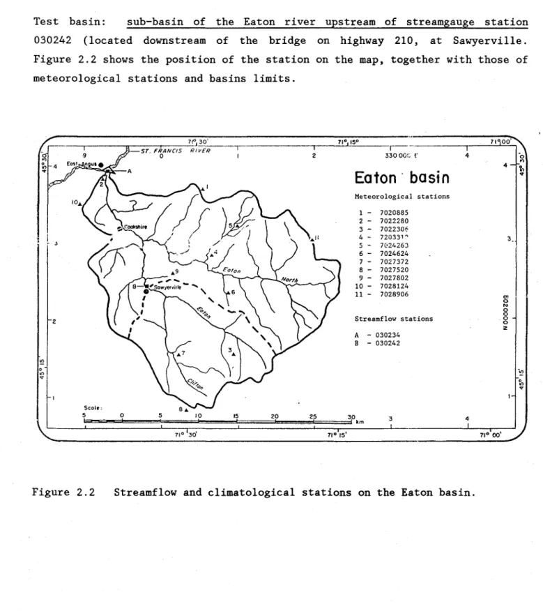
Test basin: sub-basin of the Eaton river upstream of streamgauge station

030242 (located downstream of the bridge on highway 210, at Sawyerville. Figure 2.2 shows the position of the station on the map, together with those of meteorological stations and basins limits.

71° 30' 71°.15° ST. FRANCIS RivER 1 , -0 2 33000:; r 4 ·0 '" 4 _~

Eaton basin

v Meteorological stations 1 - 7020885 2 - 7022280 3 - 7022306 4 - 720331" 3. 5 - 7(024263 1 6 - 7024624 7 - 7027372 8 - 7027520 9 - 7027802 10 - 7028124 11- 7028906 Cl 0 '" 0 0 2 Streamf10w stations 0 0 z A - 030234 B - 030242 ~ 0 .", ln .,. 0 ln .,. Scolt: 5 t;;;e, _, 0 1 5 10 1 15 1 20 1 25 1 30 1 km 3 4 710 130' ! 710"51

(19)

Are included in the data set:

topographic data:

File names and content:

Clifton.ALT: mean altitude of each square (m);

Clifton. ORI : aspect of each square to eight points of the compass,

identified 1 to 8 counterclokwise from East (=1);

Clifton.PTE: slope of each square (m/m);

Clifton.MSK: basin mask;

Clifton.NDS: information on reach ends (identification number, UTM

coordinates (m), altitude (m) and channel width (m);

Clifton.TRO: information on reaches (identification numbers for lower

and higher ends (in tha t order), Manning' s roughnes s coefficient) .

File structure for *.ALT,*.ORI,*.PTE,*.MSK:

record #1 : file type: 1.;

record #2 : number of lines, number of colums;

record tJ3 : UTM coordinates (Easting, Northing) of upper left corner,

grid size (m);

record #4: title or comment identifying the file;

record #5 to end of file: data (separated by blanks).

File structure for *.NDS:

record tH: file type: 1.;

record tn: number of reach ends;

record #3 : title or comment identifying the file;

record #4 to (3 + number of reach ends): identification number,

(20)

File structure for '1(.TRO:

record #1:

record

#12 :

record #3:

file type: 1. ;

number of reaches (= number of reach ends - 1);

title or comment identifying the file;

record #4 to (3 + number of reaches): identification numbers for

lower and higher ends, Manning's roughness coefficient.

land-use data for each square:

file name: Clifton.CLA;

file structure:

record #1: file type: 1.;

record #2: number of lines, number of columns, number of classes;

record #3: EAST, NORTH, class codes, TOTAL;

record #4 to 3 + (li x co): UTM coordinates (Easting, Northing) of

upper le ft corner, number of pixels belonging to each class, total number of pixels.

class identification and codes:

bare fields: "champ";

crops and pasture 1 : "herbe";

crops and pasture 2: "paill";

extracting areas: "gravi" ;

forested areas 1 (coniferous): "resin

_"

;

forested areas 2 (deciduous): "feuil";

highways and other impervious areas: "route";

surface waters 1: "eau1";

surface waters 2: "eau2";

urban areas: "urb" (not in use);

waste lands and bushes: "frich" and

_"

coupe ;

_"

(21)

identification of streamflow and meteorological stations available for use in the simulation:

file name: Clifton.STN:

file structure:

record #1: file type: 1. ;

record #2: number of streamflow stations, number of meteorological

stations;

record #3: title or comment identifying the file;

identification numbers for streamflow stations; identification numbers for meteorological stations. record #4:

record #5:

streamflow data (ms -1) at streamgauge station 030242 for 1973 and 1974,

beginning on the 1st of January of each year;

file name: H030242.YY (H station identification.year):

file structure:

record #1: station identification, year, number of valid values;

record #2 to 32: 366 daily streamflows. Missing data (including

February 29): -1000.

meteorological data (maximum daily air temperature, minimum daily air temperature, rainfall, snowfall), for 1973 and 1974, beginning on the 1st of January of each year, at the following stations:

7020885 Bury;

7022280 East-Angus;

7022306 Eaton 2nd Branch; 7023312 Island Brook; 7024263 Lawrence;

7024624 Maple Leaf East;

7027372 St-Isidore d'Auckland; 7027520 St-Malo d'Auckland;

(22)

7027802 Sawyerville Nord; 7028124 Sherbrooke A; 7028906 West Ditton.

file name: M7020885.YY (M station identification.year):

file structure:

record #1: station identification, year, numbers (4) of valid data

for maximum temperature, minimum temperature, rain and snow

respectively, latitude in degrees and minutes, longitude in degrees and minutes, altitude (m), station identification;

record #2 to 17: 366 maximum temperature

(OC);

record #18 to 33: 366 minimum temperature

(OC);

record #34 to 49: 366 rainfall values (10-1 _mm);

record #50 to 65: 366 snowfall values (10-1 _cm).

missing data:

temperatures: -99;

rainfall or snowfall: -1.

2.3 USING HYDROTEL (1.0)

2.3.1 Starting HYDROTEL 1.0

Your files should now be in the proper directories or sub-directories, including your own basin files or the test files.

If you are not there, first come back (change) to c:\HYDROTEL\MODEL.

Now, type "PREMOD" and the main menu will appear on the screen.

It should be mentioned at this stage that a tree structure has been developed

(23)

user should normally be able to go through all steps in the initialization process easily.

2.3.2 Main menu

The main menu contains 6 options (figure 2.3). You have to go through options

1 to 4, before choosing option 5 "RUN" to execute the progr am wi th the chosen

options. To choose an option, first go to that option using the arrows on the

keyboard. Then, push the "ENTER" key. The sub-menu needed to define that

option will appear.

When the last simulation is finished, you can go out of HYDROTEL by choosing the "End of simulation" option and pressing "ENTER".

---_._.--,

Figure 2.3 MAIN MENU l . 2 . 3. 4 . 5.

o .

Input of simulation parametersi Input of physiographic data filesi Sub-modelsi Output optionsi Runi End of simulation.

'---_

.•... _-.-...

_

..

__

...

-

_._--Main menu.

2.3.3 Sub-menu #1.0: input of simulation parameters

1

Sub-menu #1 (figure 2.4) contains 3 options. You have to select each of those

options before returning to the previous (main) menu (by selecting option "0"

followed by the "ENTER" key). Each of these options leads you to a new

(24)

...

M-A-I-N-M-E=N=U~~·-

___

--=~_.

______ ,

--l

1. SIMULATION PARAMETERS

2.

.

1 les; 3. 1. Path to files; 4. 2. Temporal parameters; 5. 3. Spatial parameters;

O.

Return to previous menu.

' - -

'----_._

...

_--_

... : .... _-_ ...

_--_.-

---Figure 2.4 Sub-menu #1.0: input of simulation parameters.

2.3.3.1 Sub-menu #1.1: paths to files

Informations on paths to files used by HYDROTEL have to be given here (figure 2.5):

MAIN MENU

1.

2. 3. 4. 5.

O.

Figure 2.5

SIMULATION PARAMETERS

1.

-r~ T;-";~'''-;

I LES

2.

3._ . . . Path to system. files:

0._ ... Path to data flles:

! ....

Basil' filename:

I

FlO : Accept

t _ .. .... _._ .. _______ _

Sub-menu #1.1: paths to files.

.. ----··l

1·

1 1 1 c:\hydrotel\model\ c:\hydrotel\basins\ c1. l f::r,n Esc: Quit .. _ _ _ _ ... _. _ _ _ _ _ _ _ _ --1

(25)

path to system files: type HYDROTEL\MODEL, section 2.2.2;

system files contain menus and programs. if you have followed instructions

You should given in

path to data files: it has been suggested in section 2.2 to group data

files in a particular sub-directory. The path to files in that

sub-directory should be given here;

basin filename: this is the name under which aIl data files for a

particular basin will be identified. As an example, the general name for

aIl data in the set furnished with the program is "CLIFTON". Particular

files are identified by "CLIFTON. '1do'(", with the stars corresponding to

letters and/or numbers identifying the specifie file.

At any time in that sub-menu you can quit the initialization process by pushing

"ESC". The paths and basin na me appearing on the screen remains in effect. No

change is made to the previously stored name.

Normally, once the information is given you want to confirm or accept it.

Press "Fla". The paths to files are stored for later use by the program and

return to the previous sub-menu #1.0 is done automatically.

2.3.3.2 Sub-menu /11.2: temporal parameters

Back to sub-menu #1.0, go to the next option "Temporal parameters" and press "ENTER" to get sub-menu #1.2 (figure 2.6):

start of simulation (YYDDD): the year (last two digits) and day (1 to 366

(table 2.1)) of the first day of the simulation;

duration (NN): the number of consecutive days in the simulation;

(26)

DAY Jan. Feb. March April May June July Aug. Sept. Oct. Nov. Dec. DAY 1 1 32 60 91 121 152 182 213 244 274 305 335 1 2 2 33 61 92 122 153 183 214 245 275 306 336 2 3 3 34 62 93 123 154 184 215 246 276 307 337 3 4 4 35 63 94 124 155 185 216 247 277 308 338 4 5 5 36 64 95 125 156 186 217 248 278 309 339 5 6 6 37 65 96 126 157 187 218 249 279 310 340 6 7 7 38 66 97 127 158 188 219 250 280 311 341 7 8 8 39 67 98 128 159 189 220 251 281 312 342 8 9 9 40 68 99 129 160 190 221 252 282 313 343 9 10 10 41 69 100 130 161 191 222 253 283 314 344 10 11 11 42 70 101 131 162 192 223 254 284 315 345 11 12 12 43 71 102 132 163 193 224 255 285 316 346 12 13 13 44 72 103 133 164 194 225 256 286 317 347 13 14 14 45 73 104 134 165 195 226 257 287 318 348 14 15 15 46 74 105 135 166 196 227 258 288 319 349 15 16 16 47 75 106 136 167 197 228 259 289 320 350 16 17 17 48 76 107 137 168 198 229 260 290 321 351 17 18 18 49 77 108 138 169 199 230 261 291 322 352 18 19 19 50 78 109 139 170 200 231 262 292 323 353 19 20 20 51 79 110 140 171 201 232 263 293 324 354 20 21 21 52 80 111 141 172 202 233 264 294 325 355 21 22 22 53 81 112 142 173 203 234 265 295 326 356 22 23 23 54 82 113 143 174 204 235 266 296 327 357 23 24 24 55 83 114 144 175 205 236 267 297 328 358 24 25 25 56 84 115 145 176 206 237 268 298 329 359 25 26 26 57 85 116 146 177 207 238 269 299 330 360 26 27 27 58 86 117 147 178 208 239 270 300 331 361 27 28 28 59 87 118 148 179 209 240 271 301 332 362 28 29 29 .,'( ₈₈ ₁₁₉ ₁₄₉ ₁₈₀ ₂₁₀ ₂₄₁ ₂₇₂ ₃₀₂ ₃₃₃ ₃₆₃ 29 30 30 89 120 150 181 211 242 273 303 334 364 30 31 31 90 151 212 243 304 365 31

(27)

MAIN MENU

~-J

1-2. 3. 4. 5. O. Figure 2.6 SIMULATION PARAMETERS 1 i

1.

2. 3.

O •

Iles; TEMPORAL PARAMETERS

... Start of simulation (YYDDD): 73

... Dur~tion (days): 30

1 ••• Time St2p (4ays): l

152

FIO: Accept Esc: Quit

._---_.

_._-_

....

_.

Sub-menu #1.2: temporal parameters.

AlI those values are entered by going to the proper line with the arrows on the

keyboard and typing the appropriate values. When this is done, accept (and

save) the values by pressing F10.

If you want to leave the menu without change, press "ESC".

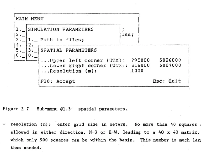
2.3.3.3 Sub-menu #1.3: spatial parameters

Back to sub-menu f/1.0, go to the next option "Spatial parameters" and press

"ENTER" to get sub-menu #1.3 (figure 2.7):

upper left corner (UTM): enter the upper left corner of the rectangular

grid containing the basin, in UTM coordinates. Note: this will be changed

in later versions of HYDROTEL to use other coordinate systems more suitable to large basins;

lower right corner (UTM): enter the lower right corner of the rectangular

(28)

1. 2. 3. 4. 5. O.

"---',

_._._-..

__

._-_._---_.

SIMULATION PARAMETERS

li

Iles; 1 1._ Path ta filesi 2 • -

r--.. --·-..

---·-·---3._ SPATIAL PARAMETERS O.

. . . UDper left corner lUTH)"

l

l" • Lo ... ·er r ight co::ner (U'I'H j ;

. . . Resolution (m): F10: Accept

_

..

_._---_.-?95000 316000 1000

Figure 2.7 Sub-menu #1.3: spatial parameters.

5026000

l

500ïOOO i

Esc: Quit

1

resolution (m): enter grid size in meters. No more than 40 squares are

allowed in either direction, N-S or E-W, leading to a 40 x 40 matrix, of

which only 900 squares can be within the basin. This number is much larger

than needed.

When this is done, accept (and save) the values by pressing "F10".

If you want to leave the menu without change, press "ESC".

Back to sub-menu #1.0 (figure 2.4), go to "Return to previous menu" and press "ENTER" to go back to the "main menu".

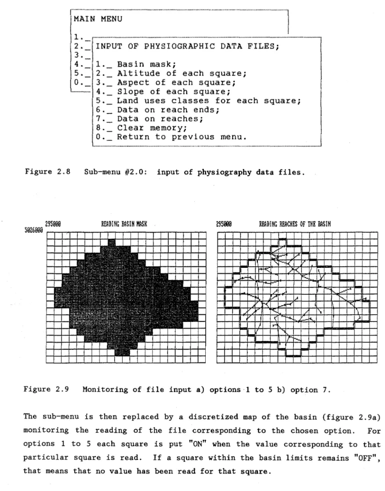
2.3.4 Sub-menu #2.0: input of physiography data files

All first seven options (figure 2.8) have to be selected, sequentially by moving to each of these options and pressing "ENTER".

(29)

r··-···-···-·· .... ,,·· .... ··_··-.. -··· .. ···-··· .. ··· ... - ... -.. -... " ... -... "" ... - ... -... ---... -... -... _ ... - ... " ... " ...

1

'MAIN MENU

1.

_1-· .... · .. ·· .... ··· .. ··· .. ·· .. ···-·· .. ·· .. ··_·_-·· ... -... -... -.... -... -... ···· .... ··· .. ·· .. · ... ·-·-·· ... ----· ... -...

-1

'2,_ INPUT OF PHYSIOGRAPHIC DATA FILES; 1

3,

4._ 1. Basin mask;

5. 2. Altitude of each square;

O. 3. Aspect of each square;

4. Slope of each square;

5. Land uses classes for each square;

6. Data on reach ends;

7. Data on reaches;

l

s.-

O. Clear memorYi Return to previous menu. 'I

... =_ ... _ ... """""""" .... "

... "

.. ,, .. ,," .. "

.. "

... """"."-"" .. "

.... ""_ .... """ .. _._" .. "

.. "".-.. "

.... _""""" .. ",,,, .. _ ... ,,"

Figure 2.8 Sub-menu #2.0: input of physiography data files.

295999 R~DING BASIN MASK 295009 ~DING ~CHES OF THE BASIN

S926BB9 ~--T"""'--"--"'--T""-'-"--"--T""-'-"--"~"'--r--T"-'--r-,..., , 1;::::' 1-'"' 1/' -"'r--K v te::. Lt5:~ li I.+--!-<- _,...

r::

y

-•

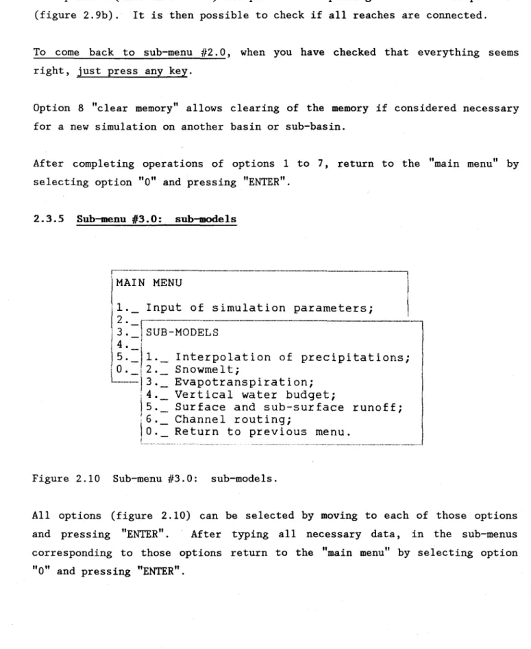
1...-1-" V 1 .... 1'-... m .... r-.; .-" f-r' 1 ""=: f ' L Il "\ '\ r-. -1<-. 2 1- 1.-' Ir r-.

Figure 2.9 Monitoring of file input a) options'l to 5 b) option 7.

The sub-menu is then replaced by a discretized map of the basin (figure 2.9a)

monitoring the reading of the file corresponding to the chosen option. For

options 1 to 5 each square is put "ON" when the value corresponding to that

particular square is read. If a square within the basin limits remains "OFF",

(30)

For option 6 (data on reach extremities), the pixels corresponding to aIl reach extremities in the basin are put "ON".

For option 7 (data on reaches) a11 pixels corresponding to reaches are put "ON"

(figure 2.9b). It is then possible to check if aIl reaches are connected.

To come back to sub-menu #2.0, when you have checked that everything seems right, just press any key.

Option 8 "clear memory" allows clearing of the memory if considered necessary for a new simulation on another basin or sub-basin.

After completing operations of options 1 to 7, return to the "main menu" by

selecting option "0" and pressing "ENTER".

2.3.5 Sub-menu 113.0: sub-models

r···_···· .. ··· __ ···_·_··· .. ···_· ... _ .. _ ... -.-._ ... _ .... -... __ .. _ ... _ ... _ .... -.-,

)MAIN MENU

1

Il._ Input of simulation parameters; \

1

2 • - r···_···_·_·_ .. ·_ .. ···_··_ ... _ .. _ ... _ ... _ ... __ .-.. _ ... __ .... _ ... _ ... _._.··_··_···_·· .. ~··· ..

I

13._I.SUB-MODELS

1 14 ! i • ' t

)5.=11._

Interpolation of precipitations; 1 i O. ,2. Snowme l t; 1

L

.. _

...

::::::j3.=

Evapotranspirationi 1

:4. Vertical water budget; 1

)5.=

Surface and sub-surface runoffi 1

·6. Channel routing; 1

1 0 •

=

Re

t

ur n

t

0

~~

=

.o..~=.~.~

... : ...

J

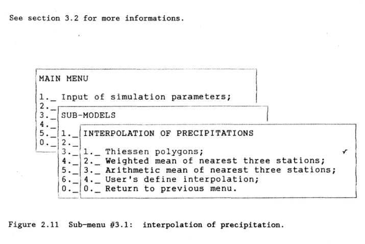
Figure 2.10 Sub-menu #3.0: sub-models.

A11 options (figure 2.10) can be selected by moving to each of those options

and pressing "ENTER". After typing a11 necessary data, in the sub-menus

corresponding to those options return to the "main menu" by selecting option

(31)

2.3.5.1 Sub-menu #3.1: interpolation of precipitation

See section 3.2 for more informations.

MAIN MENU

--1

1._ Input of simulation parameters; 1

2 • -

r .. ·· .. ···_ .. ··· .. ··· .. ··· .. ··· ... _

... :

... )

l3._!SUB-MODELS 1

i 4. 1 ;... ... ]

15.-l1.

!INTERPOLATION OF PRECIPITATIONS 1

1°.=12

_{..., . _ ' . _}₃

.=1

₁ Th' _{Iessen po ygonsi}l _y 1 ₁

14._\2._

Weighted mean of nearest three stations; 1

/5._13._

Arithmetic.mea~

of

neare~t

three stations; 'l'

16'-14.-

User's deflne InterpolatIon; 1

10'_1°'_

Return to previous menu. i

... L ... _ ... _ ... _ _ ... _ ... _ ... _ ... _ ...

J

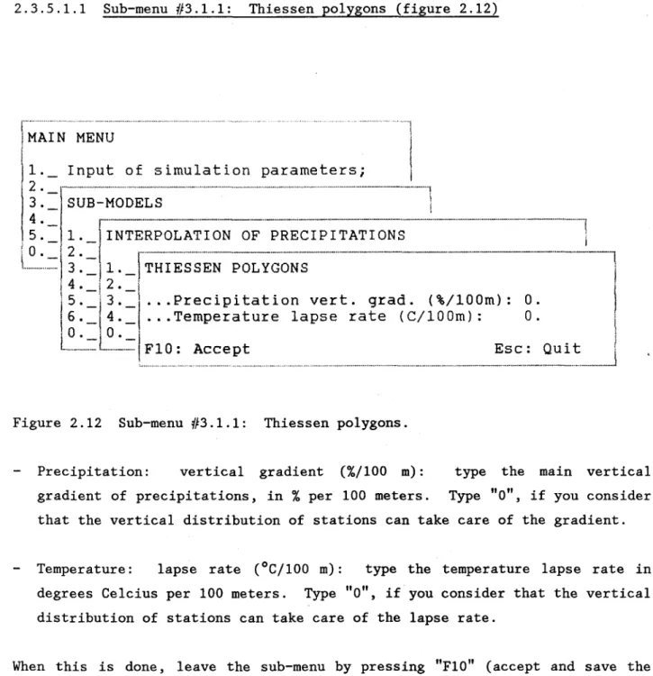
Figure 2.11 Sub-menu #3.1: interpolation of precipitation.

Three options are avai1ab1e for the interpolation of precipitations

(figure 2.11). Select one of those and press "ENTER". After typing input

values in sub-menus 3.1.1, 3.1.2 or 3.1.3, return to "sub-menu 3.0" by

se1ecting option "0" and pressing "ENTER".

I t is possible to write a user' s define interpolation function with HYDROTEL

1.0, but that wou1d require writing a1so a snow me1t subprogram. Separate and

simplified programming of both tasks (interpolation and snowme1 t) will be

availab1e in the next version of HYDROTEL. P1ease contact us, shou1d i t be

(32)

2.3.5.1.1 Sub-menu #3.1.1: Thiessen polygons (figure 2.12)

j""... ···l

IMAIN MENU ;

1 1

ll.-

Input of simulation parametersi 1

i 2. , ... " .... " ... -"'-"'-"'''1 )

3.-I

_SUB-MODELS _\ 4 •

=

1 f'''''''''-''-''-''''''''''''--'''''''''-''''-'''''''''''-''--'-'''-''-''''''''._ .. "_ ... _ .... _ ... "".""._ .. _ ... _ •. _ ... "" ...

~

.•. ",, .... _ ... " ... " ... " ... " ... , j5._11._IINTERPOLATION OF PRECIPITATIONS \

l

0 •

-1

2 •

-1

r·· ... ·

... ·

.. ·

... ··· .. ···· ... ·_ .. ·_ ... _· .... ·

... _

.... _

... _

.. _

... _-.. _

.. _

.. __ ... ,,_ ... _

....

""'''-''-''''-'''-''''-''''''''-''''-''-'''-''1

; ... 13.

_Il.

_j THIESSEN POLYGONS i

, 4 ' 2 ' ,

'/15:=\3:=11 . . . Precipitation vert. grad. (%/100m): O.

1 \6._

14._ . . . Temperature lapse rate (C/IOOm):

o.

.

!

_{... = _}

o.

l'O. "

_{.... _.=}

_{FIO: Accept} _{Esc: Quit} ₁

,

. . ... " ... ". .. ... " ... " ... " ... " ... _ ... " .. " ... " ... " .. "..1

Figure 2.12 Sub-menu #3.1.1: Thiessen polygons.

Precipitation: vertical gradient (%/100 m): type the main vertical

gradient of precipitations, in % per 100 meters. Type "0", if you consider

that the vertical distribution of stations can take care of the gradient.

Temperature: lapse rate (oC/lOO m): type the temperature lapse rate in

degrees Celcius per 100 meters. Type "0", if you consider that the vertical

distribution of stations can take care of the lapse rate.

When this is done, leave the sub-menu by pressing "F10" (accept and save the new values) or "ESC" (no change to previously stored values).

(33)

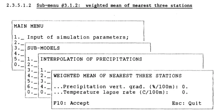
2.3.5.1.2 Sub-menu #3.1.2: weighted mean of nearest three stations

r .. ···· .. ·

IMAIN MENU ... · ... · .. · .. · ... · ... · ... · ... ·1 ! 1

11._ Input of simulation parametersi 1

; 2. , ... ···· ... ··· .... ··· ... ···· ... ··· .. ··· .. ···1

!

3.-lsUB-MODELS 1 4 • - / r ... ·_ ... · .. · _ ... · .... _ ... ·_· ... ·_ ... ·· ... · .... · ... , 1 5 ·=11._!INTERPOLATION OF PRECIPITATIONS 1

0'_1

2

_{'_i}

_!

,· .... ·

... ·

.. t!

:=/

~:=

WEIGHTED MEAN OF NEAREST THREE STATIONS . /

5'_1 3 ._

6'_14._ ... Precipitation vert. grad. (%/100m): O.

jO'_IO'_1 ...

Temperature lapse rate (C/100m):

O.

1 ... ,.,,, ... ,, ••• 1,."" ... , ... ! !

IF10: Accept Esc: Quit i

L. ... _ ... _ ... _ .. _ ... _ ... _ ...

.-1

Figure 2.13 Sub-menu #3.1.2: weighted mean of nearest three stations.

As seen in figure 2.13, this sub-menu is similar to 3.1.1. The information

given is 2.3.5.1.1 applies.

2.3.5.1.3 Sub-menu #3.1.3: arithmetic mean of nearest three stations

i

IMAIN MENU

11-_

Input of simulation parametersi 1

1₂

.-1" ... · ....

1

\3._!SUB-MODELS 1 i 4. i 1 ... •• .. · ... • ... · ... • ... • .. ••• .... • ... • ... • ... ·•· ... _ ... _ ... _ ...

_·l

f\'5.=\1._

I

IINTERPOLATION OF PRECIPITATIONS \

°'_1

2 ._

1

, .... · .... · ... · .. ·j3·_11._ Thiessen polygonsi 1 i4. '2 ... · .. ·· .. ··· ... ·· ... · ... · .... · ... 1

/5.-/3.-/ARITHMETIC MEAN OF NEAREST THREE STATIONS 1

; 6. -\ 4. -\

!O.-/O.-! ...

precipitation vert. grad. (%/100m):

O.

I.. ...

=L ... ·

.... ·=I ...

Temperature lapse rate (C/100m): O.

jF10: Accept Esc: Quit

...

(34)

As seen in figure 2.14, this sub-menu is similar to 3.1.1. The information

given in 2.3.5.1.1 applies.

2.3.5.2 Sub-menu #3.2: snowmelt

r· .. ··· .. ··· ... · .. · .. ··· .. ··· .. ··· ... ··· .. ···1

[MAIN MENU

1

Il.

Input of simulation parametersi

1

\ - 1 ) 2 ._/"" ... _ ... 1

l3._!SUB-MODELS

1 1

~

:

-11. .. ... _

... _

...

!..-....

1

jO.=)2.=!SNOWMELT

1 , ... ' 3. j i

14.=11._

Modified degree/day methodi y \

15._1\2._ User's defined snowmelti

16.

O. Return to previous menu.

! - ,

-l..~

....

:_~::~:::::::~::::~::::~=::::~:::::::::::::.::.~.:~.:

..

::::~::::~.~::::.:::~~:~::.::::

...

::::~::

.. :::.::: .. :::::::::::.:::: .. ::::: .. : ..

::::::.:~:.::::~:

..

::~

..

:::::~::::::::~~

..

:::::::::~

.... ::::; ...

I

Figure 2.15 Sub-menu #3.2: snowmelt.

Only one option is currently available for snowcover simulation and mel ting

(figure 2.15). Select it and press "ENTER". After typing input values in

sub-menu 3.2.1 (figure 2.16), return to "sub-menu 3.0" by selecting option "0"

and pressing "ENTER".

The same remarks as in 2.3.5.1 applies here, if a user decides to write his own

(35)

2.3.5.2.1 Sub-menu #3.2.1: modified degree-day method (figure 2.16)

1

---l

MAIN MENU

1._ Input of simulation parametersi

; :

=r~-~;~~

S

---l

4.

~ : ; : =rNOWM;~---l

!

:='\'

l·_rMODIFIED DEGREE/DAY M E T H O D - - -

---1

5._ 2'_1 j

6_10 __ : . . . Temp. for h:ansf. c':: 1:'3.'n into snow (l"Ie): O.

l

o._L __

j •••

Melt factor (coniferous forest) (mm/dOC): 2.

--_·-·_--·_·---1"

.Melt facto:::- (deciduous forest) (mm/dOC): 3.

l' ..

Melt factor (open areas) (mm/dOC): 4.

\ . . . Treshold tempo for melt (OC): O.

1

. . . Melt rate at snow/ground interface (mm/d): 0.5

. . . Maximum density of snowpack (hg/m3): 550

J

. . . Settlement constant: 0.1

. . . Hour zone: 2

bo:

Accept Esc: Quit

Figure 2.16 Sub-menu #3.2.1: modified degree-day method.

See section 3.3 for more informations.

Temperature for transformation of rain into snow (OC): type the threshold

temperature (OC) for the transformation of ra in into snow.

Melt factor (coniferous forest) (mm/d-OC): type melt factor for coniferous

forests, in millimeters per day and degree Celcius.

Melt fàctor (deciduous forest) (mm/d-OC): type mel t factor for deciduous

forests;

Melt factor (open areas) (mm/d-OC): type melt factor for open areas.

Threshold temperature for mel t (OC): type threshold_ temperature for mel t,

(36)

Melt rate at snow/ground interface (mm/d): type estimated mean constant melt rate at snow/ground interface, in millimeters per day.

Maximum density of snowpack (kg/m3

) :

snowpack, in kilograms per cubic meters.

type estimated maximum density of

Settlement constant: type the settlement constant (smaller than one).

Hour zone: Atlantic (1);

East (2); Center (3); Prairies (4); West (5).

2.3.5.3 Sub-menu #3.3: evapotranspiration

!" ... _ ... _ ... _ ... _ ... _ .... _ .. _ ... __ ... __ ... _ .. _ ... _ ...

-!

lMAIN MENU .

Il.

Input of simulation parameters; !

1

2 •

=

r ... _

... ··· .... ·_ .. _

.... ·· .. ·· .. · .... · ... ·· .. _

.. · ... · .. ··· .... ···· ... _

... _

.... _

... _._ .. _-.. ···· ..

_··_··...:···-1

i3._jSUB-MODELS 1

\~:=Il._

Interpolation of precipitations; \

f O. i 2. , ... _ ... _ ... _ ... _._ ... _ ... _ ... _ ... __ ... _ .... _._ ... _ ... _ .... _ .... _ ... -.. _ .... ·_· __ .... ··· .. ···--··-1

\ -1

_{, ... , 3. . EVAPOTRANSPIRATION}

-\

1

14. -1

'

15'=11 __

THORNTHWAITE potential evapotranspiration;

16-_

2 __ User's defined potential evapotranspiration;

L~

...

~

..

=

L.~

... :

...

=

...

~.=

...

~_.~.:_~_

...

~.~

...

~.:=

..

~

..

~

..

~.~.=

...

~:.~.~:

... _... ... .

(37)

Only one option is currently available for the estimation of potential

evapotranspiration (figure 2.17). Select it and press "ENTER". After typing

input values in sub-menu 3.3.1 (figure 2.18), return to "sub-menu 3.0" by selecting option "0" and pressing "ENTER".

It is possible to write a user's defined option. See section 2.5, and contact

us, eventually.

2.3.5.3.1 Sub-menu #3.3.1: input data for Thorthwaite PE (figure 2.18)

r;~IN

MENU

1

1._ Input of simulation parameters; 1

2 . -... ---- -.---

---1

3. SUB-MODELS 4._

l

5.- 1._ Interpolation of precipitations;

O.

2. -_._--

- - - - .

--- 3. EVAPOTRANSPIRATION

---_

..

_---]

~

: =

1. - ' INPUT DATA FOR - THORNTHWAI TE PE .6. 2. 1

jO'=LO.= ...

Thorn+:hwaite tnermal indl"x:

L..._ --~ ••• Mean latitude of the basin (degreesl: ..• Temporal shift parameter:

FlO: Accept

30. 45.25

80

Esc: Quit

Figure 2.18 Sub-menu #3.3.1: input data for Thorthwaite PE.

See section 3.4.1 for more informations.

Thorthwaite thermal index: type Thorthwaite thermal index.

Mean latitude of the basin (degrees): type mean latitude of the basin, in

degrees and hundredths of a degree.

Temporal shift parameter: type temporal shift parameter in days.

(38)

2.3.5.4 Sub-menu #3.4: vertical water budget

r··· .... ···· .. ···_· .... ··· .. ···_···_ .. ··· ... _

... _

... ···_· __

···1

jMAIN MENU

\1,_ Input of simulation parameters;

1

12 , - r···_···_··· .. ·· ... _ ..• _ .. __ .. _ •. _ ... _ .... _ .. _ ... _ ... _ ... _: ... ,

j3'_ISUB-MODELS

1 1~:=11.- Interpol~tion

of precipitations; 1

i 0, 1 2 • Sn 0 wme l t 1

\.. ... =

1 3 ,

=

r· ... _

.. ··· ... ···· .. · ... ···· .... ··· ... ·· .... ··· ... ·· .. ·· ... -... _

... ,

l

i 4 '_1 VERTICAL WATER BUDGET 1 j

5

,_1

11

6'_1

1 ._ CEQUEAU (modified); y

j

i

L_~;~~~_~ ~;_~_~;~_:;!~~:

1 j

Figure 2.19 Sub-menu #3.4: vertical water budget.

Only one option is currently available for the estimation of the vertical water

budget on each square (figure 2.19). Select it and press "ENTER". After

typing input values in each of the derived sub-menus, return to "sub-menu 3.0" by selecting option "0" and pressing "ENTER".

It is possible to write a user's defined option. See section 2.5 and contact

(39)

2.3.5.4.1 Sub-menu #3.4.1: input data for CEQUEAU

... "... .. .... ·· ... · ... ·· .. ··· .. ·• .... ··1

)MAIN MENU 1

Il._ Input of simulation parameters; 1

12. , ... · .... · .. ·· .. ·· .. · .. · .... ·· ... · ... ··· .... · ... · .. · .. ··· ...

1

j3.=jSUB-MODELS 1

\45'

'_j ._

-! 1 l t n erpo a lon a l t· f preclpl a lonsi " t t· 1 1

1°'_12._ Snowmelti '

\ ... __ . 1 3. r ... · ... · .. ··· .... · ... ·· ... · .... · ... ·· ... · .... ·· .... ·· .... ··· .. · ... ··· .. ··· .... ··· .. · .. 1 i

14 .=1 VERTICAL WATER BUDGET

Il

1 5 •

-1

r .. · ... · .. · .. · .. -· .. · ... · ... · ... _ ...

"''''1

16._\1·_IINPUT DATA FOR CEQUEAU 1

jO'_12'_1 l'

1... .. • ...

··1

°

'_1

1. Runoff on impervious areasi

! ... , 2 . _ Unsaturated zone reservoir; 1

13._

Saturated zone reservoir;

j4._

Lakes and marshes;

1

5._ Initial levels in reservoiri 0._ Return ta previous menu.

! ... _... ... .. ... _ .. _ ... _ ... _ ...

J

Figure 2.20 Sub-menu #3.4.1: input data for CEQUEAU.

See section 3.5 for more information.

The usual separation of the terres triaI part of the hydrologie cycle into components has been used to group the parameters of the CEQUEAU function

(figure 2.20). This should facilitate the identification of each parameter and

the estimation of realistic values, based on the user' s knowledge of the physical characteristics of the basin.

After typing aIl necessary data in the sub-menus corresponding to those options, return to "sub-menu 3.4" by selecting option "0" and pressing "ENTER".

(40)

2.3.5.4.1.1 Sub-menu #3.4.1.1: runoff on impervious areas (figure 2.21)

:~~N '=-=~i~=tlo~arame:l

2 • M ______ ... _~ .... _M._ .. ~._ ... wM .. _ _ M_M_._ .. _._._ ... __ .. -.. -... -.-... ---.. -.--.---... . 3. SUB-MODELS 4. 5. O. 1. 2. 3. 4. 5. 6. O. L, ... . Interpolation of precipitations; Snowmelti

VERTICAL WATER BUDGET

1. _l'''~~';-~;--'-;'~;-~''-'';'o R ·-··~~-Q~·~·~~-··-···-·----···-··-·-·--··-l

2._

0._1._ RUNOFF ON IMPERVIOUS AREAS;

2 .

3. 4.

.. . Depth threshold for surface runoff (mm): O.

5. F10: Accept Esc:

O. . ... --.--.--... --... - .. - ... --.-.-.. ...

---... _ ... _ ... _ .. _ .. _ .. _. ___ ... __ .... __ ._ ... _._._ .... __ . __ .. ______ - - - l

Figure 2.21 Sub-menu #3.4.1.1: runoff on impervious areas.

Quit

Depth threshold for surface runoff (mm): type the depth threshold (in

millimeters) water available for infiltration must reach, in order to produce runoff on impervious areas.

(41)

2.3.5.4.1.2 Sub-menu #3.4.1.2: unsaturated zone reservoir (figure 2.22)

r---IMAIN MENU

Il._

Input of simulation parametersi

t 2.

-C---

---=1

/ 3'_ISUB-MODELS 4._, i ~ 1 J T - .&- - _ " " , - ' ... -. ~ •• ~ • - -1 ~-- _ ! ,... •• _ 1

/O.-i2.-

s~~~~~it~/ ~.'-'

..

of p.Lt.c_~:_J.;..:.:t.!.V':~1 \ -

-~--'- ~: ~~TI~'--;;:~~DG~T

'--'ri

\

~:_ l.J~NPUT

DATA FOR

C~QU~AU

L~,~-=

20'

_.

l

l'_IUNSATUR~

ZONE RESERVOIR

2._ ,

3 . . . . Capacity of the reservoir (mm) :

4 . . . . Threshold for sub-surface runoff (mm):

5. . .. Runoff coefficient:

(mm) :

O. • •• Threshold for percolation

... Percolation coefficient: ... Maximum rate of percolated ..• Threshold for PET (mm):

water (mm/d): 75. 60. 0.35 60. 0.15 10. 60.

F10: Accept Esc: Quit

Figure 2.22 Sub-menu #3.4.1.2: unsaturated zone reservoir.

Capacity of the reservoir (mm): type the maximum depth of water which can

be storedin the reservoir (in millimeters).

Threshold for sub-surface runoff (mm): type the threshold level water must

reach before any surface runoff begin (in millimeters).

Runoff coefficient: type the runoff coefficient.

Threshold for percolation (mm): type the threshold level (in millimeters),

water must reach before any percolation to the saturated zone reservoir occurs.

(42)

Percolation coefficient: type the percolation coefficient.

Maximum rate of percolated water (mm/d): type the maximum amount

(millimeters) of percolated water allowed each day.

Threshold for PET (mm): type the threshold level (millimiters) over which

evapotranspiration occurs at potential rate.

2.3.5.4.1.3 Sub-menu #3.4.1.3: saturated zone reservoir (figure 2.23)

:A~N I:::~

of simulation

parameter~,--1

~

:

=l-~C~·~~~~-;;Ls---

·---1

4. 1

5._ 1._ Interpolation of precipitations;

a . -

r:r~~~::;

WATER BUDGET

---11

1~:-':ll.J~NPUT~ATA

FOR

C~QUEAU

---··-l

:, i 2 .

1 '._., r ' - \ . . .• 1

L __ - i U _ , l . _ runof~ on imperviou3 areas;

L.-...

-./2. - .

.----.... -.--.---.---.,

l

l~:= SATURATED ZONE RESERVOIR 1

5._ ... Outflow coefflclent: 2.e-002

'10._ ..• Fraction of PET taken in sato zone: O. - . - ..• Ref. level for fraction of PET (mm): 50.

FlO: Accept Esc: Quit

Figure 2.23 Sub-menu #3.4.1.3: saturated zone reservoir.

Outflow coefficient: type the outflow coefficient.

Fraction of PET taken in saturated zone: type the nominal fraction of

(43)

Reference level for fraction of PET (mm): type the reference level (in millimeters) for which the effective fraction of evapotranspiration taken from the saturated zone reservoir is that given above.

2.3.5.4.1.4 Sub-menu #3.4.1.4: lakes and marshes (figure 2.24)

~N

l

::--:-~-O-f-s-i-m-u-I-a-t-i-o-n-p-arame

ters

~

2. 3. 4. 5. O. SUB-MODELS 1._ Interpolation of precipitations; 2._ Snowmelt; 3'

G

-; i :

=1

:~~r~::T

w::::

-:;---I

i G

'-i 2'_1

....

_

... _-.... _---, 3._ ---,

~.

--1

0 •

_11._

Kunoff on i~pHVious areas;

2._ Unsaturated zone reservoir;

4._ LAKES AND MARSHES 5._

0._ ..• Threshold for outf1ow (mm):

... Outflow coefficient:

250 2.5e-002

FIO: Accept Esc: Quit

Figure 2.24 Sub-menu #3.4.1.4: lakes and marshes.

Threshold for outflow (mm): type the threshold level (millimeters) water

must reach before any runoff occurs from lakes and marshes.

Outflow coefficient: type the outflow coefficient.

When this is done, leave the sub-menu by pressing "F10" (accept and save the new values) or "ESC" (no change to previous1y stored values).

(44)

2.3.5.4.1.5 Sub-menu #3.4.1.5: initial levels in reservoirs (figure 2.25) ... _._ ...

_-_._

....

__

. _ - - - , HAIN HENU 1. 2. 3. 4. 5. O.

Input of simulation parameters;

,.---._._ ...•.

_

... _ ....

_-_._

...

_._---,

SUB-MODELS

1._ Interpolation of precipitations; 2._ Snowme l t;

::=rVER~.~WA~E~BU~GET--.---

__

~

!;.

1].

1 INPè1T S!,T ... FOR CEQUEAU

10 "_1 :2 __ ;

~-~-!!ù._il._ Runo~i on impervious areasi

--['2._

Unsaturated zone reservoiri

3._ Saturated zone reservoiri

~:=

-;NITIAL LEVELS IN RESERVOIR

1

0._ _{... Unsaturated zone (mm):} _{65 .} 1

... Saturated zone (mm): 30.

1~~:Lakes and marshes (mm): 250 1

C~.~ccePt Esc: Qui t-.J

Figure 2.25 Sub-menu #3.4.1.5: initial levels in reservoirs.

Unsaturated zone (mm): type the initial level of water (in millimeters) in

the unsaturated zone reservoir.

Saturated zone (mm): type the initial level of water (in millimeters) in

the saturated zone reservoir.

Lakes and marshes (mm): type the initial level of water (in millimeters) in

the saturated zone reservoir.

(45)

2.3.5.5 Sub-menu #3.5: surface and sub-surface runoff

j""." ... " ...•.. " ... " •.•• _ ... " ••• ,,_ ... ,," ... " ... " ...• - •. _" ..•. " ...•.. " .. "" .•. _ . - - - _ .• _"." ... ,

IMAIN MENU 1

Il,_ Input of simulation parameters; \

l

2 , -

f· .. · .... · .. · ... ·· .. · ... -... ·· ... · ... "· ... ·,, ... _

... -"-... -" ... ,, ... -... -... "".-... "

...

!

j3,_ SUB-MODELS 1 ! 4 ,_1 1

15,_11._

Interpolation of precipitations; 1 10,_i2 ,- Snowmelti

i

... -.. "" .. "".1

3 . - Evapotranspiration; 1

\

~

: =

r~·~~·;·~;~··

..

··~~·~··

..

···~·~~

..

=

..

~"~·~;·~~·~·

.. ·· ..

~·~~·~·;;";

.. "

.... "

.... · .. · .... · ... ···-.. "" ..

l

\~:=Il,_ Kine~atic ~ave

equation; . . y 1

... " ... 12 ,_ User s deflned runoff functlon, l'

iO._ Return to previous menu.

L ... " ... ""... ... . ... ..1

Figure 2.26 Sub-menu #3.5: surface and sub-surface runoff.

Only one option is currently available for the simulation of surface and

sub-surface runoff (figure 2.26). Select it and press "ENTER". A control "V"

appears, confirming the selection.

After typing, in sub-menu 3.5.1, the "file name" in which initial values of water in transit are stored, return to sub-menu "3.0" by selecting option "0" and pressing "ENTER".

(46)

2.3.5.5.1 Sub-menu #3.5.1: kinematic wave equation (figure 2.27)

r-... . ... ···1

IMAIN MENU 1

Il._ Input of simulation parametersi 1

1 ~ :

=

r ..

~·~~·=~·~·~~·~·~··

.... ·· .. ·· .. ···· .. ··· ... ···· .. ·· .. ···· .. ·

... _

... -... _

... _

... ··· ... ···· ..

···1

1~:=11._

Interpolation of precipitations; 1

la.

Ii 2. Snowmelt,' : J - - 1 1... ...

13._

Evapotranspiration; J 4 • - f··· .. ··· .. ···... ... "1

1

5'-1

SURFACE AND SUB-SURFACE RUNOFFi

. 6 . ' 1··· ... ···1 1

!O·=11._.KINEMATIC WAVE 1 1

,··· ...

·I~:=!l._Read

initial settings; 1 1

L.···I

a . _

Return to prev i ous menu. 1···..J

1. ... _ ... _., ..••.•••....•..•.•.•..•.•...•.•... , ... ,._ •••.•.•••. _ •.. ~ .•. , ... _ •. _ ..••• _ ... _ ... ,,_,

Figure 2.27 Sub-menu #3.5.1: kinematic wave equations.

See section 2.4.2.2 for more information. If you want to use a pre-computed

initialization file select "Read initial settings" and press "ENTER". A

control "V" will appear and the "file name" will be asked when the program is

run. Otherwise, initial runoff values are initialized to "zero". Return to

(47)

2.3.5.6 Sub-menu #3.6: channel routing

1 .. ··· .... ··· .. ·· .. ··· .. · .. ·· ... · ... ··· ... · .... · .. ·... ..

iMAIN MENU

-1

Il._ Input of simulation parameters; 1

1

~

:

=

l'''~.~.~.=.~.~.~.~.~.~

...

"""-""""""''''''''''''''''''''''''''''''''''''''''''''''''''''''''---'''''''''''''''1

1~:=ll._

Interpolation of precipitations; 1

iO._)2._

Snowmelti !

14._ Vertical water budget;

1..""""'''''''''''1 3 ._ Evapotranspirationi 1

\

~

: =

r~~'~~'~-~'~"""'~"~'~"~"~"~'~""""""""'"'''-''''''''''''''''''''''''"'''-'''--''-'''-''''''''-'''''''''''''''-''''-''-''''''''''''''''-''''''''''-''''' ... _ .. _ ... \

10 ! 1

\ ·-11

_{... ;} _{. _}M d'f' d k' ₀ ₁ _le _{lnema lC wave equa loni}t· t·

_or

1

!

12._

User's defined channel routing function; 1

)0._ Return to previous menu. 1

... _ ... _._ ... __ ... _ .. _ .... _ ... _ ... _." ... _._ ... ....1

Figure 2.28 Sub-menu #3.6: channel routing.

Only one option is currently available for the simulation of channel routing

(figure 2.28). Select it and press "ENTER". A control "V" appears, confirming

the selection.

After typing, in sub-menu 3.6.1, the "file name" in which initial values of channel water are stored, return to sub-menu "3.0" by selecting option "0" and pressing "ENTER".