Petroleum projects selection by taking the risk
into account
Fateh BELAID
1Daniel De Wolf
1,21
Institut des Mers du Nord
2HEC Ecole de gestion ULG
Universit´e du Littoral Cˆote d’Opale Universit´e du Littoral Cˆote d’Opale 21 quai de la Citadelle, BP 5528 49/79 Place du Gal de Gaulle, BP 5529 59 383 Dunkerque Cedex 1, France 59 383 Dunkerque Cedex 1, France Email: [email protected] Email: [email protected]
December 10, 2008
Abstract
Two important characteristics of petroleum exploration and pro-duction investment are the high financial amounts and uncertainties. For these reasons, the risk analysis should be implemented in the projects evaluation and the selection process. Depending on their available resources, petroleum companies choose a number of projects on the basis of some criteria: the net present value, internal rate of return, profitability index However, these criteria appear to be in-sufficient if we consider, on the one hand, the absence of risk idea which is an essential element of the petroleum industry, on the other hand the omission of the correlations and interactions between differ-ent projects. In this paper, in order to make up for the lacks of the traditional approach, we apply a variant of Markowitzs method to de-termine the efficient portfolio exploration and production projects that insure the best compromise minimum risk-maximum return under the different constraints faced by the company. A practical application of this method about selection of petroleum exploration projects in the North Sea is presented. This practical case illustrates the influence of the crude price in the choice of the portfolio.
1
Introduction
Petroleum exploration deals with many unknowns, with high risk and uncer-tainty being an inherent part of the oil and gas industry. The management of risk in oil and gas exploration has always been a difficult subject, and it is even more important in these days of high capital investment and high volatility of oil price.
This paper presents comments and some background on the use of risk analysis methods in the Oil and gas industry. Particularly attention is given to applications developed specifically for exploration and production projects selection.
The main objective is to present an application of the Markowitz theory about the investment projects selection. Wishing to present a comprehensive and simple method, that is to say, easy to apply by the decision makers in the petroleum companies. Premium evaluation criteria in investment are necessary in each step of the decision, however, the important question that needs to find an answer in this research is: how shall we use the portfolio optimization approach to make the strategic investment decision as easy as possible from a practical point of view?
In general, the funds are not sufficient to support all available investment opportunities. So the selection of portfolio projects is important. The selec-tion process objective is to choose a subset of projects that makes it possible to maximize the profits (objective) of the company meanwhile respecting the budget restriction (constraints). However, in addition to all the above con-siderations, the company should follow a strategy to ensure better returns with minimal risk.
2
Model flow for the whole procedure
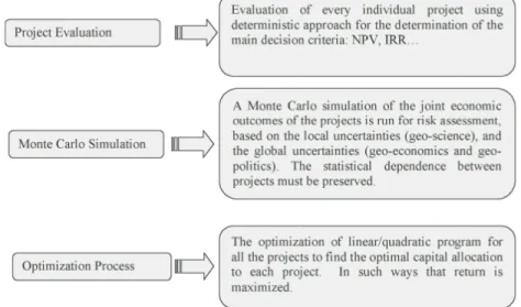
The process used to optimize EP projects portfolio is an integrated economic model. Implementation of this process involves three basic steps focused on three main stages:
1. Individual evaluation of each project by using the deterministic method to evaluate the cash-flows of exploration projects or oil production. 2. Applying Monte Carlo simulations for the assessment of projects
3. Building a portfolio optimization model for the selection of the optimal portfolios.
The construction and operation of the model are summarized in Figure 1.
Figure 1: Model flow of optimization process
The aim is to obtain an optimal rate of investment for each project to maximize the total return of the portfolio taking into account the various risks and the constraints of the company.
To do this, we compare two methods: Markowitz method with the vari-ance as a risk measure and Markowitz method with the semi-varivari-ance as risk measure.
To test the impact of the oil price volatility on the profitability of the portfolio projects, we use four models corresponding to different pricing sce-narios:
Scenario 1: low price of $25/barrel,
Scenario 2: an average price of $100/barrel, Scenario 3: high price of $200/barrel,
Scenario 4: a mixed model, where you assign a probability of occurrence of each price scenario:
• price of $25/barrel with a probability of 0.2 • price of $100/barrel with a probability of 0.4 • price of $200/barrel with a probability of 0.4
3
Markowitz portfolios optimization method
Since the seminal work of Markowitz (1952), mathematical analysis on port-folio management has grown considerably. Variance has become the most popular mathematical definition for the risk of portfolio selection. Markowitz shows how rational investors can construct optimal portfolios under condi-tions of uncertainty. The average and variance of a portfolios return represent the benefit and risk associated with the investment. Several researchers have developed a variety of models to handle risk using variance as risk measure. For example, Hlouskova (2000), Chopra (1998), Chow (1994)
Variance is a useful measure of risk. In calculating variance, positive and negative deviations from the average are equally weighted. In fact, decision-makers are often more worried about downside risk the risk of failure. A solution to this problem is to determine the efficient set of portfolios by using another risk measure. Semi-variance overcomes this problem by mea-suring the probability and distribution below the average return. Several models have been developed using semi-variance as risk measure, for exam-ple, Markowitz (1993), Grootveld (1999), Homaifar (1999), Huang (2008) In the average downside risk investment models the variance is replaced with a downside risk measure then only results below a certain point contribute to risk.
3.1
Basic set of notation
For indices, we use, i and j to denote the different EP projects and t for the years. Parameters are denoted:
N total number of projects (14 in our application); E number of exploration projects (5 in our application); EN P Vi the expected return of project i
(given by the Monte Carlo simulation);
σij coefficients of the covariance matrix defined for project i and j
(given by the Monte Carlo simulation);
Ωij coefficients of the semi-covariance matrix defined for project i and j
(given by the Monte Carlo simulation); Ri reserves of project i;
Pi production of project i;
Ii investment of project i;
Pmin t minimum targeted production for year t;
Rmin minimum reserves required from the selected portfolio
(500MM bbl);
Imax total capital available to investment (5,000 $MM);
α capital enrichment for the selected portfolio (0.2); ρmin the desired level of return for the selected portfolio
(900 $MM);
λ coefficient reflecting the risk aversion factor of the investor (0 ≤ λ ≤ 1);
β the fraction of the total investment allocated to exploration product (20 %).
3.2
Markowitz model with variance as risk measure
The decision variables are simply :
Xi = the fraction of the project i invested in the portfolio
Both decision variables may vary within specific ranges (0% to 100%) lim-ited by estimated constraints (technical, physical and budget constraints). Supposing we can participate in the project at any level.
A portfolio optimization was conducted for a group of 14 Exploration and Production projects in the North Sea under risk consideration, resulting in an efficient frontier. In this case risk was estimated by the variance as calculated across Monte Carlo simulation. In this model the objective function is a linear combination of net present value against risk (variance).
Model: Max (NPV VAR): max z1 = (1 − λ) N X i=1 EN P ViXi− λ N X i=1 N X j=1 σijXiXj
Under the constraints: ∀i = 1, 2, ...N , ∀t = 2013,...2017 0 ≤ Xi ≤ 1 N X i=1 IiXi ≤ Imax N X i=1 RiXi ≥ Rmin N X i=1 EN P ViXi ≥ ρmin X i∈E IiXi ≥ B N X i=1 IiXi N X i=1 PitXi ≥ Pmin,t
Its a quadratic model which consists in maximizing the objective function (return risk). For each value of λ, we determine the value Xi (fraction of
each project invested in the portfolio) and also the corresponding portfolio return and risk. The latter are elements of the efficient frontier curve. We get the whole efficient frontier curve by resolving this problem for different values of λ using iteration (λ0 = 0; λ1 = 0,01; λ2 = 0,02; λ3 = 0,03; λ4 =
0,04; λ5 = 0,05; λ6 = 0,06; λ7 = 0,07; λ8 = 0,08; λ9 = 0,09; λ10 = 0,10; λ11
= 0,15; λ12 = 0,20; λ13 = 0,30; λ14 = 0,40; λ15 = 0,50; λ16 = 0,60; λ17 =
0,70; λ18 = 0,90; λ19 = 0,99; λ20 = 1).
3.3
Markowitz model with semi-variance as risk
mea-sure
Variance penalizes both extreme gains and extreme losses. In contrast, semi-variance stimulates the selection of projects with a low probability of returns below a critical value like the expected return. Therefore, we propose a new optimization model: the portfolio projects with semi-variance as risk
measure. Each portfolio in the frontier represents a set of projects satisfying minimum levels of production, tolerable operational and maintenance costs, precedence relations between projects, and a limited budget.
Likewise, according to prospect theory (Tversky and Kahneman 1991), in-vestors see a loss as riskier than a gain of the same amount, which contradicts the use of variance when extreme potential gains and losses are equivalent (Choobineh and Branting 1986). Semi-variance overcomes this problem by measuring the probability and dispersion below the average value. Thats why the optimization framework is now modified to minimize semi-variance (instead of variance) for a given expected NPV.
The model of optimization with semi-variance as risk measure is written below:
Mod`ele : Max (NPV-SVAR) : max z1 = (1 − λ) N X i=1 EN P ViXi− λ N X i=1 N X j=1 ΩijXiXj
Under the constraints: ∀i = 1, 2, ...N , ∀t = 2013,...2017 0 ≤ Xi ≤ 1 N X i=1 IiXi ≤ Imax N X i=1 RiXi ≥ Rmin N X i=1 EN P ViXi ≥ ρmin X i∈E IiXi ≥ B N X i=1 IiXi N X i=1 PitXi ≥ Pmin,t
4
Results of the model
Economic evaluation models are created for each project in Excel file models and evaluated under concession contracts. The resolution of the different quadratic optimization models under Markowitzs method is obtained using GAMS software.
4.1
Markowitz method with variance as risk measure
In this part, to get the curve of the efficient frontier, we vary the values of λ (risk tolerance) in the [0, 1].
4.1.1 Scenario 1(price of $25/barrel):
With this scenario, we obtained 10 different optimal portfolios. The table in Appendix A gives us the contents of each portfolio.
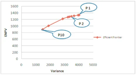
Figure 2: Efficient frontier for a price of $ 25/barrel
The portfolio P1 obtained for values λ1, λ2, λ3 and λ4 is the most
prof-itable portfolio with an ENPV= $ 1,336.04 million, and most risky with a variance of 4,019.66 and investment of $ 5,000 million. The same portfolio would have been selected with the traditional method of selecting portfolio (taking the projects in descending order of their expected ENPV). In con-trast, P10 portfolio corresponding to λ13 to λ20, the portfolio is less risky
with the lowest NPV ($ 900 million), a variance of 1,472.35 and an invest-ment of $ 3,462.56 million. In this portfolio, all projects are selected with the exception of project EXP 9, which is very logical because its NPV is negative (-37,12).The P4 portfolio reduces the risk portfolio with a 9% yield loss of $23.91 million. The project EXP9 was selected in any portfolio, which it is very risky, contrary to projects EXP7 and EXP8 that are selected among all portfolios. From these results, we can build the efficient frontier (see Figure 2).
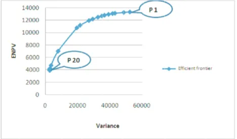
4.1.2 Scenario 2(an average price of $100/barrel):
We apply Markowitz method to our fourteen projects with the price of oil at $100/barrel. The number of efficient portfolios is 20. The portfolio P1 is the most risky with a yield of $13,326.95 million, a variance of 52,271.98, and an investment of $5,000 million. Note that this portfolio is the one chosen by the traditional method. On the contrary, the portfolio P20 is less risky with a NPV of $3 913.17 million, a variance of 2,612.63, and an investment of $ 1,938.45 million. The remaining results are presented in the table in Appendix A. The resulting efficient frontier is presented by the Figure 3.
Figure 3: Efficient frontier for a price of $100/barrel
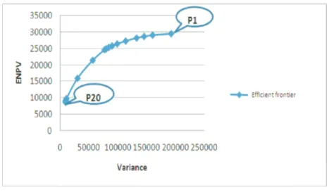
4.1.3 Scenario 3 (high price of $200/barrel):
With the price of $200/barrel, we get the same number of efficient portfolios as in scenario 2. The portfolio P1 is the most profitable with an EVAN $29,464.91 million, a variance of 193,029.29 and an investment of $4,995.594 million. The yield corresponds to the portfolio selected with the traditional method of the maximum expected NPV, except that its composition is not the same. The project EXP7 which has not been selected before is in the new portfolio with a fraction of 0.34%. The results are presented in Appendix A. The resulting efficient frontier is traced in Figure 4.
Figure 4: Efficient frontier for a price of $200/barrel
4.1.4 Scenario 4 (average price):
After applying the model on the three price scenarios, we apply it on the expected NPV result of these three scenarios. Altogether, we get 20 effi-cient portfolios. The results are presented in the table in Appendix B. After reading the latter, we note that the portfolio P 1 is the most profitable with a return of $17 355.14 million, a variance of 98,334.55, and an investment of $4995.78 million. The portfolio is the same as the one selected with the traditional method, with a small difference in composition: for example, the project EXP 7, which is selected with a ratio of 24% was not chosen by the traditional method, as well as the project EXP 4 selected with a fraction of 0.89% while it had been selected in full by the traditional method. The graph in Figure 5 presents the resulting efficient frontier of the model.
4.2
Maximizing performance with the semi-variance as
a risk measure
As in Markowitz et al. (1993), we calculate the portfolios NPV as follows:
SV (R) =
N
X
i=1
Figure 5: Efficient frontier for the average price
The semi-covariance between projects is defined as follows:
Ωij = N X i=1 N X j=1 [min(V ANi− EN P Vi, 0) · min(V ANj − EN P Vj, 0)]/N
4.2.1 Scenario 1(price of $25/barrel):
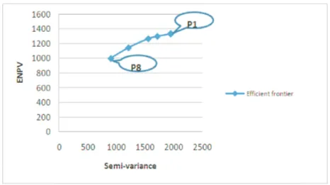
By using the semi-variance as a risk measure, we get optimal portfolios 8, i.e. less than the model of variance, because for different λ, we obtain portfolios with a similar performance and the same risk. The portfolio P1 is the most risky with a semi-variance of 1,950.16 and a return of $ 1 336.04 million. P8 is the least risky portfolio with a semi-variance of 908.11, a return of $1 000 million, and an investment of $3 874.90 million. The results are presented in the table in Appendix B.
The efficient frontier is presented on the graph in Figure 6. We notice that it is different from that obtained with the use of variance as a measure of the risk. For a similar return the risk is not so high. It is due to the fact that semi-variance considers as risk only the returns below the average contrary to variance which does not make a difference between the returns below and above extremes.
Figure 6: Efficient frontier for a price of $25/barrel
4.2.2 Scenario 2 (oil price of 100 $/barrel):
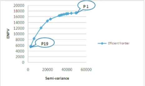
The application of the method of Markowitz with the semi variance as a measure of risk on this scenario provides us with 19 optimal wallets. P1is the riskiest portfolio with a semi-variance of 29,136. 00, an output of $13,326.95 million and an investment of $5,000 million, while P19 is the least risky wallet with a semi-variance of 1,938.45 and an expected NPV of $ 3,913.17 million and one investment of $1,938.45 million. It is noticed that the composition of P1 is the same as the portfolio selected with the traditional method for the same price scenario. The results are presented in Figure 7.
4.2.3 Scenario 3 (oil price of $200 /barrel):
The use of the semi-variance as a measure of the risk on this scenario gives us 19 optimal portfolios with compositions close to those obtained with the use of variance. P1 is the the most risky portfolio with a semi-variance of 97,956.37, a $29 489.20 million dollar return and a $5,000 million dollar investment. It corresponds to the same portfolio as that obtained with the traditional method. P2 is the less risky portfolio, with a semi-variance of 4,927. 53, a NPV of $8,721.27 million, and an investment of $1,947.04 million. The results are represented in Figure 8.
Figure 7: Efficient frontier for a price of $100/barrel
4.2.4 Scenario 4 (average NPV):
This average scenario, gave us 19 optimal portfolios. The compositions of which are different from those obtained with variance as a measure of the risk, on the other hand the returns are close. P1 is the most risky portfolio with a semi-variance of 49,882. a NPV of $17,367 million, and an investment of $5,000 million (it is the same portfolio as the one obtained with the classical method). P2 is the least risky portfolio with a semi-variance of 2,484, a NPV of $5,116 million, and an investment of $1,952 million, the latter reduces the risk of 95 % and the investment of 60 % ($3 047 million) with a loss of 70 % return ($12 250 million). The efficient frontier with the results of the model is presented in Figure 9.
Figure 9: Efficient frontier for the average price
4.3
Comparison of both resulting efficient frontiers of
the maximization of variance and semi variance
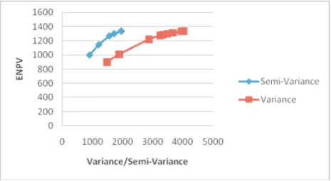
To illustrate the impact of variance and semi-variance as a risk measure, we draw the resulting efficient frontier of both measures on the same graph for the various price scenarii (see Figures 10, 11, 12, 13 below). We notice that the efficient frontiers of the models with semi-variance as a measure of risk are different from those of variance as risk measure. We note that for the
same level of return, semi-variance corresponds to a lower risk. However, with the decrease of the risk, the difference or the dispersal between both curves becomes smaller.
Figure 10: Scenario 1: Oil price of $25/barrel.
5
Conclusion
The model is articulated on the following three main stages:
• cash-flow analysis of projects by the deterministic calculations by using the NPV criteria;
• cash-flow analysis of projects by the stochastic calculations using the Monte Carlo simulation to calculate NPV ;
• Selection of the optimal portfolio of projects using the Markowitz method , by using two different statistics as risk measure (variance and semi-variance).
The portfolio optimization method based on the Markowitz method al-lows the decision-makers to see the marginal contribution of every project to the portfolio, so to define the portfolios of optimal projects and the best rate of participation in every project, this method, contrary to the classical selection methods, analyzes the projects by considering the
Figure 11: Scenario 2: Oil price of $100/barrel.
Figure 13: Scenario 4: Average oil price .
various aspects of the risk and the various correlations which exist between the various projects. This allows us to better identify the projects risk, quan-tify risk, and limit the investment failures. The method allows to determine: • The allocation of capital as well as the distribution of the production
and the returns for every project;
• The adequate strategies of investment, which answer the expected ob-jectives, and respect the budgetary constraints of the company.
The use of variance as risk measure in the optimization penalizes projects for upward as well as downward potential. We can overcome the problem by using semi-variance in the definition of the problem of optimization. Semi-variance concentrates only on the reduction of the losses, without taking into account risks of the extreme potential earnings, what makes it particu-larly desirable for the asymmetrical distributions of probability as those of the profitability of petroleum and gas industries. This approach allows the portfolio managers to define the risk in an adequate way according to the objectives and the constraints which are imposed on him concerning the re-turn on its portfolio. This study demonstrates that an explicit analysis of uncertainties and interdependencies in evaluating the risks of EP projects improves the quality of investment decision-making.
A key feature of the methodology outlined here is its flexibility, its abil-ity to incorporate different sources of uncertainty into its simple three-step process: (1) variable identification (2) projects evaluation, and (3) quadratic optimization.
References
[1] Al-Harthy, M. H. (2007). Stochastic oil price models: Comparison and impact, Eng. Econ. 52(3) pp 269-284.
[2] Babusiaux D. (1990), D´ecision d’investissement et calcul ´economique dans l’entreprise, Paris, Economica et Technip.
[3] Babusiaux D. (2005), P´etrole: quelles productions et quels prix `a l’avenir ?, P´etrole et Techniques, No. 456, pp 39-44.
[4] Babusiaux D., Pierru A., (2002), Decision d’investissement et cr´eation de la valeur, exercices, probl`emes et ´etudes de cas, Ed. Technip, Paris. [5] Babusiaux D., et al (2007), Oil and Gas Exploration and Production,
IFP Publication, Edition TECHNIP, Paris.
[6] Choobineh, F., D. Branting. 1986. A simple approximation for semivari-ance. Eur. J. Oper. Res. 27(3) 364370.
[7] Chow K., Denning K.C. (1994), On variance and lower partial moment betas: The equivalence of systematic risk measures, Journal of Business Finance and Accounting 21, pp 231-241.
[8] Grootveld, H., W. Hallerbach (1999). Variance vs downside risk: Is there really that much difference? Eur. J. Oper. Res. 114(2) 304319.
[9] Homaifar G., Graddy D.B. (1990), Variance and lower partial moment betas as alternative risk measures in cost of capital estimation: A defense of the CAPM beta, Journal of Business Finance and Accounting 17, pp 677-688.
[10] Huang, X. (2008), Portfolio selection with new definition of risk. Eur. J. Oper. Res. 1(1) pp 351-357.
[11] Markowitz, H. (1952), Portfolio selection. J. Financ. 7(1), pp 77-91. [12] Markowitz, H. (1959), Portfolio Selection: Efficient Diversification of
Investment. John Wiley & Sons, New York.
[13] Markowitz, H., P. Todd, G. Xu, Y. Yamane (1993), Computation of mean-semivariance efficient sets by the critical line algorithm, Ann. Oper. Res. 45(1), pp 307-317.
[14] Tversky, A., D. Kahneman. (1991), Loss aversion in riskless choice: A reference-dependent model. Q. J. Econ 106(4) 10391061.
A
Results of the of Markowitz method with
the variance as risk measure
A.1
Scenario 1(price with $25/barrel)
P 1 P 2 P 3 P 4 P5 P 6 P 7 P 8 P 9 P 10 λ (λ1, λ4) (λ5) (λ6) (λ7) (λ8) (λ9) (λ10) (λ11) (λ12) (λ13, ...λ20) EN P V 1 336,04 1 335,83 1 331,96 1 312,13 1 296,7 1 283,58 1 273,08 1 221,26 1 009,04 900 VAR 4 019,66 4 015,26 3 952,78 3 666,31 3 475,23 3 333,4 3 233,05 2 867,56 1 879,82 1 472,35 Invest. 5 000 5 000 4 995,44 5 000 5 000 5 000 4 997,56 4 991,39 3 881,92 3 462,56 EXP1 1 1 1 1 1 1 1 1 1 0,93 EXP2 1 1 1 1 1 1 1 0,86 0,63 0,55 EXP3 0 0 0 0 0 0 0 0,16 0,13 0,11 EXP4 1 0,98 0,99 0,98 0,97 0,96 0,95 0,9 0,65 0,57 EXP5 0,59 0,63 0,68 0,7 0,92 0,73 0,73 0,75 0,55 0,48 EXP6 0 0 0 0 0 0 0 0,09 0,11 0,1 EXP7 1 1 1 1 1 1 1 1 1 1 EXP8 1 1 1 1 1 1 1 1 1 1 EXP9 0 0 0 0 0 0 0 0 0 0 EXP10 0 0 0 0,11 0,2 0,26 0,31 0,44 0,33 0,29 EXP11 1 1 1 1 1 1 1 1 0,9 0,79 EXP12 0 0 0 0 0 0,11 0,19 0,43 0,33 0,29 EXP13 1 1 1 1 1 1 1 0,97 0,7 0,61 EXP14 1 1 0,97 0,88 0,8 0,74 0,69 0,55 0,4 0,35
A.2
Scenario 2 (oil price 100 $/barrel)
P 1 P 2 P 3 P 4 P5 P 6 P 7 P 8 P 9 P 10 λ (λ1) (λ2) (λ3) (λ4) (λ5) (λ6) (λ7) (λ8) (λ9) (λ10) EN P V 13 326,95 13 262,31 13 130,01 13 076,30 12 956,12 12 811,90 12 697,75 12 497,50 12 195,73 11 954,31 VAR 52 271,98 48 537,89 43 093,57 41 562,56 39 091,16 36 591,30 34 940,76 32 520,30 29 259,51 26 952,65 Invest. 5 000,00 4 997,45 4 992,98 5 000,00 5 000,00 5 000,00 4 994,04 5 000,00 5 000,00 5 000,00 EXP1 1,00 1,00 1,00 1,00 1,00 1,00 1,00 1,00 1,00 1,00 EXP2 0,48 0,49 0,6 0,72 0,72 0,68 0,65 0,64 0,63 0,62 EXP3 0 0 0 0 0,05 0,15 0,24 0,31 0,9 0,43 EXP4 1 0,83 0,95 1 1 1 0,96 0,93 0,9 0,89 EXP5 1 1 1 1 1 1 0,99 0,94 0,38 0,87 EXP6 1 1 1 1 1 1 1 1 1 1 EXP7 0 0,76 1 1 1 1 1 1 1 1 EXP8 1 1 1 1 1 1 1 1 1 1 EXP9 1 1 1 1 1 1 1 1 1 1 EXP10 0 0 0 0 0,09 0,18 0,25 0,32 0,37 0,41 EXP11 1 1 1 1 1 1 1 0,95 0,84 0,75 EXP12 1 1 1 1 1 1 1 1 1 1 EXP13 1 1 0,99 0,96 0,89 0,8 0,74 0,7 0,68 0,65 EXP14 1 0,93 0,73 0,65 0,58 0,51 0,46 0,43 0,41 0,39 P 11 P 12 P 13 P 14 P 15 P 16 P 17 P 18 P 19 P 20 λ (λ11) (λ12) (λ13) (λ14) (λ15) (λ16) (λ17) (λ18) (λ19) (λ20) EN P V 11 199,96 10 781,01 7 022,16 4 718,48 4 230,82 4 124,93 4 049,30 3 948,46 3 916,38 3 913,17 Var 21 457,16 19 433,57 7 817,18 3 442,91 2 771,45 2 683,22 2 641,80 2 614,59 2 612,65 2 612,63 Invest. 5 000,00 5 000,00 3 261,31 2 189,74 1 984,15 1 984,66 1 956,97 1 942,99 1 938,45 1 938,45 EXP1 0,93 0,80 0,48 0,30 0,25 0,22 0,20 0,17 0,16 0,16 EXP2 0,6 0,6 0,37 0,24 0,21 0,21 0,2 0,2 0,19 0,19 EXP3 0,58 0,67 0,42 0,27 0,25 0,26 0,26 0,26 0,27 0,27 EXP4 0,84 0,82 0,49 0,32 0,32 0,34 0,35 0,38 0,38 0,38 EXP5 0,78 0,74 0,45 0,29 0,26 0,25 0,24 0,24 0,23 0,23 EXP6 0,98 0,94 0,58 0,37 0,31 0,28 0,26 0,24 0,23 0,23 EXP7 1 1 1 0,78 0,71 0,71 0,71 0,7 0,7 0,7 EXP8 1 1 1 1 1 1 1 1 1 1 EXP9 1 1 1 0,73 0,59 0,52 0,47 0,4 0,37 0,37 EXP10 0,53 0,6 0,37 0,24 0,22 0,23 0,23 0,23 0,24 0,24 EXP11 0,48 0,35 0,21 0,13 0,09 0,06 0,05 0,02 0,01 0,01 EXP12 1 0,99 0,59 0,38 0,31 0,28 0,25 0,22 0,21 0,21 EXP13 0,59 0,56 0,34 0,22 0,19 0,19 0,19 0,18 0,18 0,18 EXP14 0,33 0,3 0,18 0,12 0,11 0,11 0,11 0,11 0,11 0,11A.3
Scenario 3 (oil price to $200 /barrel)
P 1 P 2 P 3 P 4 P5 P 6 P 7 P 8 P 9 P 10 λ (λ1) (λ2) (λ3) (λ4) (λ5) (λ6) (λ7) (λ8) (λ9) (λ10) ENPV 29 464,91 29 024,44 28 623,73 28 162,15 27 254,45 26 401,29 25 791,89 25 334,84 24 949,62 24 619 Var 193 029,29 160 842,24 145 948,43 133 047,73 11 4107,2 99 319,12 90 497,35 84 833,21 80 680,66 77 524 Invest 4 995,594 5 000 5 000 4 997,547 5 000 5 000 5 000 49 90,885 5 000 5 000 EXP1 1 1 1 1 1 1 1 1 0,97 0,92 EXP2 0,39 0,61 0,65 0,6 0,58 0,57 0,57 0,56 0,56 0,56 EXP3 0 0 0,13 0,28 0,39 0,46 0,52 0,56 0,59 0,62 EXP4 0,95 1 1 0,95 0,91 0,88 0,85 0,84 0,83 0,82 EXP5 1 1 1 0,94 0,86 0,81 0,77 0,74 0,72 0,71 EXP6 1 1 1 1 1 1 1 1 1 1 EXP7 0,34 1 1 1 1 1 1 1 1 1 EXP8 1 1 1 1 1 1 1 1 1 1 EXP9 1 1 1 1 1 1 1 1 1 1 EXP10 0 0 0,09 0,25 0,35 0,42 0,47 0,5 0,54 0,56 EXP11 1 1 1 1 0,86 0,71 0,61 0,53 0,46 0,41 EXP12 1 1 1 1 1 1 1 1 1 1 EXP13 1 0,96 0,85 0,74 0,69 0,65 0,63 0,61 0,6 0,59 EXP14 1 0,71 0,59 0,49 0,44 0,41 0,38 0,36 0,35 0,34 P 11 P 12 P 13 P 14 P 15 P 16 P 17 P 18 P 19 P 20 λ (λ11) (λ12) (λ13) (λ14) (λ15) (λ16) (λ17) (λ18) (λ19) (λ20) ENPV 21 434,81 15 939,24 9 823,18 9 362,22 9 148,59 9 006,17 8 904,45 8 768,81 8 725,65 8 721,34 Var 56 954,76 30 392,84 11 259,24 10 333,5 10 066,51 9 947,83 9 892,12 9 855,52 9 852,9 9 852,88 Invest 4 482,98 33 21,59 2 029,58 1 978,08 1 970,38 1 956,381 1 959,21 1 948,78 1 934,93 1 947,04 EXP1 0,7 0,5 0,29 0,25 0,23 0,21 0,2 0,18 0,18 0,18 EXP2 0,49 0,34 0,2 0,19 0,18 0,18 0,18 0,18 0,17 0,17 EXP3 0,61 0,43 0,25 0,25 0,26 0,26 0,26 0,26 0,26 0,26 EXP4 0,71 0,5 0,29 0,32 0,34 0,35 0,36 0,38 0,38 0,38 EXP5 0,59 0,42 0,24 0,23 0,22 0,22 0,21 0,21 0,21 0,21 EXP6 0,98 0,7 0,41 0,36 0,33 0,31 0,3 0,28 0,27 0,27 EXP7 1 1 0,75 0,74 0,73 0,73 0,73 0,73 0,73 0,73 EXP8 1 1 1 1 1 1 1 1 1 1 EXP9 1 1 0,68 0,55 0,47 0,42 0,38 0,33 0,32 0,32 EXP10 0,54 0,38 0,22 0,22 0,23 0,23 0,23 0,23 0,23 0,24 EXP11 0,26 0,19 0,11 0,07 0,05 0,03 0,02 0,01 0 0 EXP12 0,97 0,69 0,4 0,34 0,31 0,29 0,27 0,25 0,24 0,24 EXP13 0,5 0,35 0,21 0,2 0,2 0,2 0,2 0,19 0,19 0,19 EXP14 0,27 0,19 0,11 0,11 0,11 0,11 0,12 0,12 0,12 0,12A.4
Scenario 4 (average NPV)
P 1 P 2 P 3 P 4 P5 P 6 P 7 P 8 P 9 P 10 λ (λ1) (λ2) (λ3) (λ4) (λ5) (λ6) (λ7) (λ8) (λ9) (λ10) EN P V 17 355,14 17 113,72 17 008,06 16 741,05 16 522,13 15 972,15 15 533,75 15 204,96 14 949,23 14 730,72 Var 98 334,55 82 459,21 78 140,29 70 885,84 66 178,96 56 737,72 50 391,44 46 316,73 43 553,42 41 469,82 Invest 4 995,78 5 000,00 5 000,00 5 000,00 4 999,28 4 997,77 5 000,00 5 000,00 5 000,00 4 993,17 EXP1 1 1 1 1 1 1 1 1 1 0,97 EXP2 0,51 0,67 0,83 0,8 0,77 0,75 0,74 0,73 0,72 0,72 EXP3 0 0 0 0,14 0,27 0,36 0,43 0,48 0,52 0,55 EXP4 0,89 0,91 1 0,97 0,92 0,88 0,86 0,84 0,82 0,81 EXP5 1 1 1 0,9 0,82 0,77 0,73 0,7 0,68 0,66 EXP6 1 1 1 1 1 1 1 1 1 1 EXP7 0,24 1 1 1 1 1 1 1 1 1 EXP8 1 1 1 1 1 1 1 1 1 1 EXP9 1 1 1 1 1 1 1 1 1 1 EXP10 0 0 0 0,14 0,26 0,34 0,4 0,44 0,48 0,5 EXP11 1 1 1 1 1 0,85 0,72 0,62 0,55 0,49 EXP12 1 1 1 1 1 1 1 1 1 1 EXP13 1 0,95 0,89 0,79 0,72 0,68 0,65 0,62 0,61 0,59 EXP14 1 0,75 0,63 0,54 0,47 0,43 0,4 0,83 0,36 0,35 P 11 P 12 P 13 P 14 P 15 P 16 P 17 P 18 P 19 P 20 λ (λ11) (λ12) (λ13) (λ14) (λ15) (λ16) (λ17) (λ18) (λ19) (λ20) EN P V 14 020,69 10 616,19 6 630,19 5 547,11 5 404,05 5 308,68 5 240,56 5 149,73 5 120,83 5 117,94 Var 36 263,00 20 063,64 7 567,59 5 286,99 5 108,17 5 028,69 4 991,39 4 966,88 4 965,12 4 965,11 Invest 5 000,00 3 767,27 2 351,95 2 006,69 1 981,24 1 959,76 1 959,79 1 952,98 1 961,98 1 960,47 EXP1 0,8 0,57 0,34 0,26 0,23 0,21 0,2 0,18 0,17 0,17 EXP2 0,71 0,51 0,3 0,25 0,24 0,24 0,23 0,23 0,23 0,23 EXP3 0,66 0,48 0,28 0,25 0,25 0,25 0,25 0,25 0,26 0,26 EXP4 0,79 0,57 0,33 0,31 0,33 0,35 0,36 0,37 0,38 0,38 EXP5 0,62 0,44 0,26 0,21 0,21 0,2 0,2 0,19 0,19 0,19 EXP6 1 0,76 0,45 0,35 0,32 0,3 0,29 0,27 0,26 0,26 EXP7 1 1 0,86 0,73 0,73 0,72 0,72 0,72 0,72 0,72 EXP8 1 1 1 1 1 1 1 1 1 1 EXP9 1 1 0,75 0,56 0,48 0,43 0,39 0,34 0,33 0,32 EXP10 0,6 0,43 0,25 0,22 0,22 0,22 0,23 0,23 0,23 0,23 EXP11 0,31 0,22 0,13 0,08 0,06 0,04 0,03 0,01 0 0 EXP12 1 0,77 0,45 0,35 0,31 0,28 0,27 0,24 0,23 0,23 EXP13 0,56 0,4 0,24 0,2 0,2 0,19 0,19 0,19 0,19 0,19 EXP14 0,31 0,22 0,13 0,11 0,11 0,11 0,11 0,12 0,12 0,12B
Maximizing return with the semi-variance
as risk measure
B.1
Scenario 1(price with $25/barrel)
P 1 P 2 P 3 P 4 P5 P 6 P 7 P 8 λ (λ1, ...λ7) λ8 λ9 λ10 λ11 λ12 λ13 (λ14, ...λ20) EN P V 1 336,04 1 335,99 1 335,86 1 335,76 1 301,04 1 268,61 1 144,69 1 000 Semi-Var 1 950,16 1 949,57 1 948,22 1 947,27 1 715,75 1 559,22 1 214,22 908,11 Invest. 5 000,00 5 000,00 4 997,18 4 997,53 4 991,64 5 000,00 4 534,89 3 874,90 EXP1 1 1 1 1 1 1 1 1 EXP2 1 1 1 1 1 1 0,76 0,64 EXP3 0 0 0 0 0 0 0,15 0,12 EXP4 1 1 0,98 0,97 0,97 0,94 0,79 0,65 EXP5 0,59 0,6 0,62 0,64 0,72 0,74 0,65 0,54 EXP6 0 0 0 0 0 0 0,19 0,16 EXP7 1 1 1 1 1 1 1 1 EXP8 1 1 1 1 1 1 1 1 EXP9 0 0 0 0 0 0 0 0 EXP10 0 0 0 0 0,17 0,32 0,38 0,31 EXP11 1 1 1 1 1 1 1 0,87 EXP12 0 0 0 0 0 0,26 0,41 0,34 EXP13 1 1 1 1 1 1 0,87 0,72 EXP14 1 1 1 1 0,82 0,68 0,49 0,4