Registration algorithm optimized for simultaneous localization and mapping

R W UNIVERSITE DE

Ei£J SHERBROOKE

Faculty of Engineering

Department of Electrical Engineering and Computer Engineering

REGISTRATION ALGORITHM OPTIMIZED FOR

SIMULTANEOUS LOCALIZATION A N D M A P P I N G

ALGORITHME DE REFERENCEMENT OPTIMISE POUR LA LOCALISATION ET LA CARTOGRAPHIE SIMULTANEES

Master's Thesis in Applied Science

Speciality: Electrical Engineering

Jury composition:

Frangois Michaud

Michel Lauria

Dominic Letourneau

Frangois POMERLEAU

1*1

Library and

Archives Canada

Published Heritage

Branch

Bibliotheque et

Archives Canada

Direction du

Patrimoine de I'edition

Your file Votre reference ISBN: 978-0-494-49567-4 Our file Notre reference ISBN: 978-0-494-49567-4

NOTICE:

The author has granted a

non-exclusive license allowing Library

and Archives Canada to reproduce,

publish, archive, preserve, conserve,

communicate to the public by

telecommunication or on the Internet,

loan, distribute and sell theses

worldwide, for commercial or

non-commercial purposes, in microform,

paper, electronic and/or any other

formats.

AVIS:

L'auteur a accorde une licence non exclusive

permettant a la Bibliotheque et Archives

Canada de reproduire, publier, archiver,

sauvegarder, conserver, transmettre au public

par telecommunication ou par Plntemet, prefer,

distribuer et vendre des theses partout dans

le monde, a des fins commerciales ou autres,

sur support microforme, papier, electronique

et/ou autres formats.

The author retains copyright

ownership and moral rights in

this thesis. Neither the thesis

nor substantial extracts from it

may be printed or otherwise

reproduced without the author's

permission.

L'auteur conserve la propriete du droit d'auteur

et des droits moraux qui protege cette these.

Ni la these ni des extraits substantiels de

celle-ci ne doivent etre imprimes ou autrement

reproduits sans son autorisation.

In compliance with the Canadian

Privacy Act some supporting

forms may have been removed

from this thesis.

Conformement a la loi canadienne

sur la protection de la vie privee,

quelques formulaires secondaires

ont ete enleves de cette these.

While these forms may be included

in the document page count,

their removal does not represent

any loss of content from the

thesis.

Canada

Bien que ces formulaires

aient inclus dans la pagination,

il n'y aura aucun contenu manquant.

Resume

Construire des cartes dans un environnement inconnu tout en gardant un suivi de sa posi-tion actuelle est une etape majeure dans la realisaposi-tion d'un robot pouvant se deplacer de fagon autonome et securitaire. Au cours des 20 dernieres annees, la methode de localisa-tion et cartographie simultanees (Simultaneous Localizalocalisa-tion And Mapping, SLAM) est de-venue un sujet de grand interet en robotique. L'idee de base est de combiner l'information proprioceptive mesurant les deplacements du robot avec l'information exteroceptive sur Penvironnement afin de minimiser l'erreur globale de positionnement. Puisque le robot est en mouvement dans son environnement, l'information exteroceptive provient de differents points de vue, et ces informations doivent etre exprimees dans le meme referentiel afin qu'elles puissent etre fusionnees. Ce precede est appele referencement. L'algorithme de referencement Iterative Closest Point (ICP) a fait ses preuves dans plusieurs applications de reconstruction de modeles 3D et a recemment ete applique au SLAM. Cependant, le SLAM possede des contraintes en termes de temps reel et de robustesse qui sont differentes des applications de modelisation 3D, laissant place a une optimisation specialised pour des applications de cartographie realisees par un robot.

Apres une revue de litterature sur les approches de SLAM actuellement disponibles, ce memoire introduit une nouvelle variante de referencement appelee Kd-ICP. Cette tech-nique de referencement diminue l'erreur creee par le desalignement de deux nuages de points de fagon iterative, sans devoir extraire des elements environnementaux specifiques. Les resultats presentes demontrent que la nouvelle methode de rejet de points utilisee permet d'atteindre un referencement plus robuste a de grandes erreurs initiales de po-sitionnement. Des experiences avec des environnements simules et reels suggerent que l'algorithme Kd-ICP est plus robuste comparativement aux methodes actuelles. De plus, le Kd-ICP demeure assez rapide pour les applications en temps reel, tout en etant capable de gerer l'occlusion des senseurs et le recouvrement partiel de cartes.

Pouvoir references deux cartes locales rapidement et de fagon robuste ouvre la porte a beaucoup d'opportunites en SLAM. II devient alors possible de minimiser l'accumulation d'erreurs sur la position du robot, de fusionner l'information exteroceptive locale afin de diminuer la memoire utilisee lorsque le robot repasse souvent au meme endroit, et d'etablir les contraintes necessaires a la diminution de l'erreur globale lors de la creation d'une carte.

Mots-cle: ICP, kd-tree (arbre de k dimensions), registration (referencement), scan

Abstract

Building maps within an unknown environment while keeping track of the current position is a major step to accomplish safe and autonomous robot navigation. Within the last 20 years, Simultaneous Localization And Mapping (SLAM) became a topic of great interest in robotics. The basic idea of this technique is to combine proprioceptive robot motion information with external environmental information to minimize global positioning errors. Because the robot is moving in its environment, exteroceptive data comes from different points of view and must be expressed in the same coordinate system to be combined. The latter process is called registration. Iterative Closest Point (ICP) is a registration algorithm with very good performances in several 3D model reconstruction applications, and was recently applied to SLAM. However, SLAM has specific needs in terms of real-time and robustness comparatively to 3D model reconstructions, leaving room for specialized robotic mapping optimizations in relation to robot mapping.

After reviewing existing SLAM approaches, this thesis introduces a new registration vari-ant called Kd-ICP. This referencing technique iteratively decreases the error between mis-aligned point clouds without extracting specific environmental features. Results demon-strate that the new rejection technique used to achieve mapping registration is more robust to large initial positioning errors. Experiments with simulated and real environments sug-gest that Kd-ICP is more robust compared to other ICP variants. Moreover, the Kd-ICP is fast enough for real-time applications and is able to deal with sensor occlusions and partially overlapping maps.

Realizing fast and robust local map registrations opens the door to new opportunities in SLAM. It becomes feasible to minimize the cumulation of robot positioning errors, to fuse local environmental information, to reduce memory, usage when the robot is revisiting the same location. It is also possible to evaluate network constrains needed to minimize global mapping errors.

Remerciements

Mes recherches furent possibles grace au support financier du Conseil de recherche en sci-ences naturelles et genie du Canada (CRSNG) de meme que du programme des Chaires de Recherche du Canada (CRC). Jc voudrais egalement remercier la Fondation de l'Universite de Sherbrooke de m'avoir octroye une bourse de soutien aux recherches en traitement d'images.

Je veux premierement remercier mon directcur de these, Francois Michaud, qui fut une grande source de motivation par son dynamisme et son interet pour mes travaux. Je suis aussi redevable a la dynamique equipe du laboratoire LABORIUS pour leur aide durant mes deux annees a leur cote, et egalement pour les savantes discussions de l'heure du diner. Je remercie particulierement Frangois Ferland qui m'a offert un support technique des plus emcaces. J'aimerais egalement souligner le support de Claude et Mireille Guay durant mes etudes universitaires a Sherbrooke. Finalement, je tiens a remercier Marie-Eve Garneau pour avoir ete la pour moi, et pour avoir appris a apprecier les robots (et les ninjas, et les zombies...).

'The roots of education are bitter, but the fruit is sweet."

Contents

1 I N T R O D U C T I O N 1

2 S L A M A P P R O A C H E S 4

2.1 A Short History of SLAM . 4

2.2 Bayes' Rule 6

2.3 Sensors 6

2.3.1 Proprioceptive 6

2.3.2 Exteroceptive 7

2.4 Available SLAM Solutions 9

2.4.1 Algorithms 9

2.4.2 Libraries 11

2.5 Environments 13

2.5.1 Case study 1: Minerva 13

2.5.2 Case study 2: RoboX 15

2.6 Discussion 17

3 E X P E R I M E N T A L S E T U P 20

3.1 Optimization 20

4 K d - I C P 32

4.1 INTRODUCTION 33

4.2 Map Registration Using ICP 35

4.3 Kd-ICP 38

4.4 Experimental Results 41

4.5 Conclusion and Future Work 45

4.6 ACKNOWLEDGMENTS 46

5 M A P P I N G R E S U L T S 47

5.1 Mapping of a Large Environment 47

5.2 Mapping of a Simulated Environment 50

5.3 Mapping of a Cluttered Environment 50

5.4 Discussion 53 References 63 A Conceptual Networks 64 B Error Propagation 67 B.l Position Calculation 68 B.2 Covariance Propagation 70

List of Figures

1.1 General scheme for mobile robot navigation systems [76] 2

2.1 Conceptual network of research work on SLAM 5

2.2 Minerva platform [81] 14

2.3 Minerva's representation of Smithsonian museum [81] 15

2.4 RoboX's representation of the Robotics exhibition at Expo.02 [75] 16

2.5 Information flow for SLAM layer representation 18

2.6 Maximum likelihood error relaxation example 18

3.1 Test environment for ICP optimization 23

3.2 Example of a registration validation 24

3.3 Translation and rotation error during registration 24

3.4 Block diagram of the SLAM process implemented for validation of Kd-ICP. 25

3.5 Visualization system 26

3.6 Hierarchical data structure used in the validation system 27

3.7 Referential configuration put in place for the validation system 28

3.8 Impact of data structures on information reduction 29

3.9 Robotic platforms used for validation 30

4.2 Features combination results 42

4.3 Rejection comparison results 43

4.4 Robustness of ICP variants 44

4.5 Outdoor map realized with hundreds of local registrations only 46

5.1 Corridors map after correction 48

5.2 Corridors map before correction 49

5.3 Mapping of a simulated apartment in Player/Stage 51

5.4 Mapping of a cluttered environment 52

A.l Conceptual networks of SLAM 65

List of Tables

2.1 Available SLAM libraries . 13

3.1 Sensor specifications 31

4.1 Comparison of ICP variants 38

4.2 Timing results of Kd-ICP in real environments 45

L E X I C O N

Acronymes Definitions

AI Artificial Intelligence

ARNL Autonomous Robotic Navigation & Localization AMCL Adaptive Monte-Carlo Localization

CARMEN CARegie MEllon Navigation toolkit DOF Degree Of Freedom

EM Expectation Maximization EIF Extended Information Filter EKF Extended Kalman Filter GPL General Public License

H-SLAM Hierarchical Simultaneous Localization And Mapping HRI Human-Robot Interaction

ICP Iterative Closest Point

ICRA International Conference on Robotics and Automation IMU Inertia Measurement Unit

IR InfraRed range finder

ISRR International Symposium on Robotics Research LGPL Lesser General Public License

ML Maximum Likelihood

NDT Normal Distribution Transform RANSAC RANdom SAmple Consensus RBPF Rao Blackwellized Particle Filter SEIF Sparce Extended Information Filter SICK SICK laser range finder

SIFT Scale Invariant Feature Transform

SJPDAF Sample-based Joint Probabilistic Data Association Filters SLAM Simultaneous Localization and Mapping

SURF Speeded Up Robust Features SVN SubVersioN

T J T F Thin Junction Tree Filter

UMBmark University of Michigan Benchmark UKF Unscented Kalman Filter

UTM Hokuyo UTM-30LX laser range finder URG Hokuyo URG-04LX laser range finder ViPR Visual Pattern Recognition

Chapter 1

I N T R O D U C T I O N

Mobile robotic platforms are, by definition, robots having the capabilities of moving from one point to another without being physically attached to its environment, as opposed to static manipulators used for instance by the automotive industry in assembly lines. Thus, mobile robotic platforms navigate in unpredictable environments to accomplish useful tasks. Reactive approaches using only the robot's perceptual space make it possible to deal with highly dynamic environments. However, no anticipation and planning beyond this perceptual space is possible. To overcome this limitation, the robot must create its own representation of the environment. This requires the robot to have two concurrent capabilities: localization and mapping. A navigation scheme proposed by Siegwart et

al. [76] using those capabilities is illustrated in Figure 1.1. Starting from a specific

position in the environment, sensors collect data (e.g., position, color, texture) about objects surrounding the robot in order to use this information to derive its location in the world. What is sensed in the robot's perceptual space serves as a local map of its world, and subsequent local maps can be used to localize the robot and map the environment into a more global representation of the world (also known as global map). The problem of positioning a robot while building a map is now known as Simultaneous Localization

And Mapping (SLAM). A .global map can then be used by a path planner to derive a

path from the robot's position to a goal location, and provide navigation commands to the robot to avoid obstacles.

One key process in SLAM is the ability to align subsequent local maps with each other, a process known as registration. Simply stated, registration takes as inputs two misaligned but overlapping set of data (or point clouds) in cartesian space (derived from two local maps) and tries to find the translational and rotational transformations to align them.

Localization and Mapping

1

map-c

Sensing Acting Actuator

commands Path Execution

M o t i o n C o n t r o l

Figure 1.1: General scheme for mobile robot navigation systems [76]

With the robot moving, those point clouds are taken from different locations in time, making them somehow different but related. The Iterative Closest Point (ICP) algorithm reveals to be an interesting approach for registration, because it does so without prior landmark extractions (e.g., lines, circles, arcs, corners [88], [2]). This algorithm is used in 3D modeling tasks using a laser range finder moved manually around an object [46],

[18], [25], [74], [26], [35]. However, using ICP in SLAM requires to overcome two main limitations not currently addressed in ICP variants: 1) points clouds taken from two different viewpoints have less overlaps compared to 3D modeling tasks, mostly because of occlusions; 2) the robot's operating environment is more difficult to disambiguate. These limitations affect the robustness of ICP used in registration for SLAM.

Therefore, the research question of this work is How to improve robustness of registration

applied to SLAM?. The scientific hypothesis that we want to validate is that

percep-tual enhancement (e.g., combining multiple sensory modes to determine the position of the robot in its environment) should lead to improved robustness of ICP optimized for SLAM, leading to a new algorithm called Kd-ICP. To better situate the role of registration in SLAM, Chapter 2 presents a literature review of SLAM. Chapter 3 describes our exper-imental setup used to develop and validate Kd-ICP which consists of two environments: a simulated environment, covering a wide range of situations to test for optimizing and refining Kd-ICP; real robots, to validate our algorithm using a SLAM context application for testing in real conditions. Chapter 4 presents the paper submitted to IEEE

Interna-tional Conference on Robotics and Automation, the leading conference in robotics. This paper explains Kd-ICP for registration in SLAM and demonstrates its performances in terms of robustness and timing performances. Chapter 5 expands on additional results obtained with Kd-ICP, showing how perceptual enhancements can lead to the creation of global maps integrating a richer set of data, and highlighting additional advantages of our approach.

Chapter 2

SLAM A P P R O A C H E S

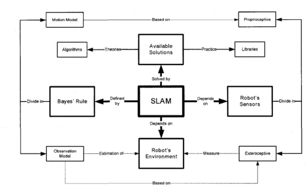
The problem of Simultaneous Localisation And Mapping (SLAM) for an autonomous mobile robot is stated as follows: starting from an initial position, a mobile robot travels through a sequence of positions and obtains a set of sensory data at each position. The goal for the mobile robot is to process the sensory data to produce an estimate of its position while concurrently building a map of the environment [28]. Figure 2.1 presents the four main concepts behind SLAM: Bayes' Rule is a probabilistic theorem used on stochastic motion and observation (or environment) models, based on two types of Robot's Sensors, proprioceptive (internal to the robot: accelerometers, gyroscopes, etc.) and exteroceptive (for perception of the Robot's Environment: laser range finders, cameras, etc.), which are used differently depending on the Available Solutions.

In this chapter, Section 2.1 provides a brief history of early developments in SLAM to explain what were the first concerns of researchers and how rapidly the field grew. In Section 2.2, the role of Bayes' rule in SLAM is explained. Then, experiments done using different sensors are discussed in Section 2.3. Section 2.4 presents a quick survey of currently available solutions to SLAM. Lastly, an overview of two case studies of indoor SLAM applications is presented in Section 2.5.

2.1 A Short History of SLAM

Work on SLAM started when probabilistic methods were introduced, both in robotics and artificial intelligence (AI) [28]. At the 1986 IEEE Robotics and Automation Conference held in San Francisco, a number of researchers were looking for solutions to localization

Motion Model

Algorithms ^ Theori

es-Bayes' Rule _{• by "} Defined

Observation

Model -Estimation of—

Available Solutions Solved by SLAM Depends on

i

Figure 2.1: Conceptual network of research work on SLAM.

and mapping as separate problems. Key players emerged with publications related to mapping [77, 27] and localization [6, 21]. Soon a link between the current robot's posi-tion error and relative posiposi-tion of observed landmarks was established, leading to the first theoretical presentation of a joint solution requiring correlation computations of a huge state vector including the vehicle pose and every landmark locations [53]. However, com-putation and convergence problems raised enough doubts at that time, and thus did not convince the robotics community that it was the right way to solve the problem. Almost 10 years passed until the first SLAM session was held at the 1999 International Sympo-sium on Robotics Research (ISRR). From that point on, an exponential workforce has been deployed to work on SLAM. The 2000 IEEE International Conference on Robotics and Automation (ICRA) Workshop on SLAM attracted 15 researchers and focused on issues such as algorithmic complexity, registration (data association) and implementation challenges. The following SLAM workshop at ICRA 2002 attracted 150 researchers with a broad range of interests and applications. The 2002 SLAM Summer School, in Stockholm, brought all the key researchers together with some 50 Ph.D. students from around the world and was a tremendous success. SLAM summer schools keep on going on a two years basis (2004 in Toulouse and 2006 in Oxford), and registrations are now limited to a fixed number of participants due to the growing number of applicants.

2.2 Bayes' Rule

Authors often compare SLAM to a chicken-and-egg problem [15, 44]. In fact, if the pose of the robot is always known during mapping, building maps is relatively easy. On the other hand, if a map is available, determining the robot's poses can be done efficiently. All significant attempts to solve this problem are directly or indirectly based on Bayes' rule which is defined as follow:

p(A\B) = rip(B\A)p(A) (2.2.1)

To quickly illustrate this probabilistic inference, imagine that A is the robot position and

B is the location of a door. Equation (2.2.1) indicates that it is possible to find the

probability p(A\B) that the robot is at a certain position knowing where is the door by multiplying three terms: p(B\A), the probability of the door location assuming that we know where the robot is; p(A), the probability of the robot's location; and rj, a normalizer that ensures a valid probability distribution. Probabilities in localization and mapping are used to take into consideration sensor noise from two categories of sensors: exteroceptive and proprioceptive. Exteroceptive sensors are used to create an observation model, while proprioceptive sensors affect the motion model. Therefore, Equation (2.2.1) needs to be evaluated twice to find the joint probability of those two models. The complete equation formulation can be found in Robotic Mapping: A Survey [80].

2.3 Sensors

Sensors are used to provide data about the robot's state and its operating environment. They can be categorized based on the type of information they return. On one hand,

proprioceptive sensors measure internal parameters to the robot, such as motor speed,

inertia, batterie level, etc. On the other hand, exteroceptive sensors acquire information about the environment (e.g., sounds, obstacle distances, colors).

2.3.1 Proprioceptive

Proprioceptive sensors in SLAM are used to determine a robot's motion model, focusing more closely on the localization aspect of SLAM. Estimating a robot's position from a

previously known location by using direction, speed and time is called dead reckoning. This navigation method is used in ships, aircraft, automobiles, rail engines and more recently in robots. In the literature, dead reckoning for mobile robots is also named

odometry.

Even though several sensors can be used for odometry, wheel encoders are frequently used due to their low cost and reliability. The UMBmark (University of Michigan Benchmark) [13] technique presents a protocol that tracks and manually corrects systematic errors based on wheel rotations. More recently, a generalization of this method with the addi-tion of stochastic error extracaddi-tion has been presented [50]. A logical extension to those protocols is proposed by Martinelli [55], by integrating an auto-calibration method to SLAM.

Other sensors helping odometry are available on the market, such as an Inertia Mea-surement Unit (IMU), which usually includes accelerometers and gyroscopes, to provide rotational velocities and linear accelerations over three axis, for a total of six degrees of freedom (DOF). Unfortunately, accelerometers need to be integrated twice to yield a po-sition, while gyroscope output needs to be integrated once to give orientation. Results indicate that using only an IMU is not appropriate for localization because the error is unbounded over time and grows faster than wheel encoders [9]. Another alternative is to use an electronic compass which directly gives the robot heading based on the earth's magnetic field. However, power lines or steel structures can cause large distortion on such readings. Nevertheless, it as been proven that since no proprioceptive sensors are perfect, uncertainty on position estimates can be decreased by fusing several sources of sensory data [10, 52].

2.3.2 Exteroceptive

Exteroceptive sensors are used in feature extraction for mapping. They can be divided in two categories: range finding and bearing-only. Bearing-only refers mostly to cameras, which give precise rotation readings but not much on depth, which is better perceived using range finding sensors. The use of both kinds of sensors for navigation started almost at the same time [6, 17], but because of limited computing power, most of the relevant solutions only using range finding.

Early implementations based on range finding are limited either by range or precision. Because most of the available robotic research platforms like the Nomad 150, Pioneers,

or Magellan include sonars for obstacles avoidance, a lot of publications present mapping results using sonars [82, 85, 93, 79]. Different SLAM algorithms were even compared on the same platform using sonars [90]. Unfortunately, sonar arrays suffer from phantom features creation in mapping [51], which limits their efficiency in SLAM. Recently, sonars used in SLAM were revitalized with their use in autonomous undersea vehicles [62].

The accessibility and reasonable cost of 2D laser range finders made them increasingly popular in mobile robotics. For example, laser range finders have been used for lines extraction [64], map building [45, 44, 43], and localization [20]. Moreover, different SLAM algorithms using laser range finders were tested on the same platform [12, 41]. Laser range finders bring many advantages over other sensors: they provide dense and more accurate range data compared to sonars; they have high sampling rates, high angular resolutions, long range at high resolution. Drawbacks are mainly their weight, higher cost and energy consumption. Recently, Hokuyo released their URG model, a light and low energy laser range finder, but with a maximum range of 4 meters and limited detection for low reflectivity obstacles. Recently, Hokuyo released their UTM model that offers better performance with a 30 meters range, and was presented on a lunar rover by the Tohoku University at the IEEE International Conference on Robotics and Automation 2008 Robot Challenge.

In the last years, bearing-only sensors received an increasing interest from the SLAM community. Processing power is increasing, and new vision-based algorithms developed for the movie industry can be adapted for real-time processing. 3D SLAM using a single camera are presented in [23, 24]. Promising results were obtained using a small number of landmarks (around 100) but limited in range, and tested without odometry inputs. Nister

et al. [65] focused on localization with an outdoor vehicle using stereo cameras. Finally,

a full solution covering localization and mapping is presented by Mouragnon et al. [59]. They present a fast and accurate method to estimate a vehicle's motion using a calibrated monocular camera. The method also gives a 3D reconstruction of the environment at using Harris corners and Random Sample Consensus (RANSAC) for features extraction.

Finally, mixed solutions using bearing-only and range finder sensors have also been tested. An algorithm for relocation is proposed by Ortin et al. [68] based on 2D laser scans map from which 3D textured planes are extrapolated. Results showed that the proposed algo-rithm outperforms both laser-only and vision-only algoalgo-rithms. Nevertheless, the publica-tion focusses only on relocapublica-tion, which is only a part of the SLAM problem, and does not mention computation requirements. Another mixed solution approach consists of using ceiling features to reduce ambiguity of 2D scans to help the robot operating in a museum

when it is not able to detect any walls for its localization [81]. There is also Folkesson et

al. [32] that used the same idea to create topological maps.

2.4 Available SLAM Solutions

Many solutions to SLAM can be found in the literature, and most of them are presented independently of sensor configurations or environments, with some making available com-plete libraries of their solutions.

2.4.1 Algorithms

It is difficult to categorize the work conducted in relation to SLAM because some of them focus either on localization or mapping optimizations, while others address one or several challenges related to SLAM. A good presentation of global SLAM solutions is presented by Grisetti et al. [40], as follows.

The estimation techniques for the SLAM problem can be classified according to their underlying basic principles. The most popular approaches are extended Kalman fil-ters (EKFs), maximum likelihood (ML) techniques, sparse extended information filfil-ters (SEIFs), and Rao Blackwellized particle filters (RBPFs). The effectiveness of the EKF approaches comes from the fact that they estimate a full correlation between landmark maps and robot poses. Their weakness lies in the strong assumptions that have to be made on the robot's motion model and sensor noise. Moreover, in the basic framework, the landmarks are assumed to be uniquely identifiable.

Thrun et al. [83] propose a SEIF method based on the inverse of the covariance matrix so that measurements can be integrated efficiently. Eustice et al. [30] present an improved technique to accurately compute the error-bounds within the SEIF framework, thus re-ducing the risk of becoming overly confident. Paskin [70] present a solution to the SLAM problem using Thin Junction Trees Filter (TJTF). This reduces the complexity compared to EKF-based approaches, because thinned junction trees provide a linear-time filtering operation.

Murphy [61] introduces Rao-Blackwellized particle filters (RBPF) as an effective mean for SLAM. Each particle in a RBPF represents a potential trajectory of the robot and a map of the environment. The framework has been subsequently extended by Montemerlo et al.

[58] for approaching the SLAM problem with landmarks, an approach called FastSLAM-2.0. To learn accurate grid maps, Hahnel et al. [43] present an improved motion model that reduces the number of required particles. A combination of the approach of Hahnel

et al. and Montemerlo et al. has been presented by Grisetti et al. [39], which extends

the ideas of FastSLAM-2.0 [58] to the gridmap case. They also present an approximative solution to RBPF-based mapping, which describes how to draw particles and how to represent the maps of the particles so that the system can be executed significantly faster using less memory resources [40].

An alternative approach is to use a Maximum Likelihood algorithm that computes a map by constructing a network of relations [54]. The relations represent the spatial constraints between the robot's poses. The main difference with RBPFs is that the Maximum Like-lihood approach can only track a single trajectory distribution of the robot. It computes the solution by minimizing the least square error introduced by the spatial constraints. The fastest solution [38] proposes a method minimizing 4,700 constraints in 11 seconds. However, this timing is obtained without considering computation time required to create those constraints.

Key research challenges for SLAM algorithms [80, 8] are defined as follow :

Measurement noise. The measurement errors are statistically dependent. This means

that the error on the position of a feature in the environment depends not only on exteroceptive sensor but also on odometry errors. Since odometry accumulates errors over time, this can cause unbounded misinterpretations of reality. This corresponds to one of the main problems to solve in SLAM.

High dimensionality. The more complex an environment is, the more features are

needed to reduce the uncertainty of a location. Even a detailed 2D floor plan can produce a lot of points. Therefore, statistics must be applied to all those features, which usually limits real-time performance capability depending on the size of the map. Line extraction is one way to reduce dimensionality and improve real-time capability. Nguyen et al. [64] present a comparison between six line extraction ap-proaches and show that Split-and-Merge and Incremental techniques are superior in terms of speed and correctness. They also propose a more compact solution for mapping [63]. For vision, Folkesson et al. [33] present M-space landmarks which can be considered as an abstraction of features dealing with constraints and sym-metries. Features are represented as points, horizontal lines and walls. Researches also used Scale-Invariant Feature Transform (SIFT) [87] and Speeded Up Robust

Features (SURF) [60] in SLAM based on cameras. At an higher level, sparsification of feature calculation [30] by using the inverse covariance matrix and submaps [14] can reduce considerably the computational complexity.

Registration. If sensor measurements are taken at different points in time, it can be

difficult to determine if they correspond to the same physical object in the world. Registration is needed during all the mapping process, but problems are highly augmented during a close loop situation or in the case of the kidnapped robot (i.e., physically take the robot from one location to put it in another). Registration techniques can be used with landmarks (e.g., lines, circles, arcs, corners) [88], [2], Normal Distribution Transform (NDT) [47] or Iterative Closest Point (ICP) [11].

D y n a m i c environment. Most of the algorithms rely on the assumption that only the

robot pose is time variant, which is usually not true. As an example, a robot giving tours in an exhibition will mostly detect people moving around it. Building maps without taking this into account can lead to drastic failures. Hahnel et al. [44, 45] were able to identify spurious measurements and track multiple people in the mapping process using Sample-based Joint Probabilistic Data Association Filters

(SJPDAF).

2.4.2 Libraries

Most of the main contributors in the SLAM community provide their libraries at no cost to other researchers, and even few commercial products are available like ARNL and ERSP 3.2. ARNL from ActivMedia [1] is a localization solution based on Monte Carlo / Markov technique (like R B P F but without mapping). It comes with a navigation module and is limited to SICK laser range finders. ERSP 3.2 from Evolution Robotics [71] provides a Software Development Kit for navigation, vision with Visual Pattern Recognition (ViPR) and interaction. A submodule called vSLAM uses vision to build a map, which is used for localization by recognizing visual features using that map. Moreover, Evolution Robotics claims to propose the first-ever, truly robust solution to robot kidnapping with vSLAM. However, no publications presenting results and comparaisons were found. Recently, Karto Robotics l proposes a C + + SDK (Software Development Kit) specialized in map

gener-ations. In addition to the SDK, Karto offers free map generation services which can be directly computed on their server.

On the open-source side, CARMEN 0.6.4 (CARegie MEllon Navigation toolkit )[56, 57] from Carnegie Mellon University is a collection of software modules for mobile robot control. It provides basic navigation primitives including mobile platform and sensor control, logging, obstacle avoidance, Monte-Carlo localization using a particle filter, path planning, and mapping. All modules related to SLAM use SICK laser range finders only. CARMEN is written in C and is licensed under the General Public Licence (GPL) license. Designed and implemented by Andrew Davison, SceneLib [22] is a generic SLAM library with a modular approach to specification of robots and sensor types. However, it also has specialized components to permit real-time vision-based SLAM with a single camera

(MonoSLAM), and the design is optimized towards this type of application. SceneLib 1.0

is an open-source C + + library licensed under the Lesser General Public License (LGPL). Another library is the CAS Robot Navigation Toolbox [3]. Not really created for on-board applications, CAS provides a useful GNU GPL licenced Matlab toolbox for robot localization and mapping. The Player Project [36, 37], including Player 2.0.3, Stage 2.0.3 and Gazebo 0.7.0, offers an interface to real robots and simulation over IP network. Player is designed to be language and platform independent, and it includes an Adaptive Monte-Carlo Localization (AMCL) implementation based on Fox et al. algorithm [34]. Client program can run on any machine that has a network connection to the robot, and it can be written in any language that supports T C P sockets. Languages currently supported on the client-side are C + + , Tel, Java, and Python.

Finally, it is possible to find source code made available by researchers. Tim Bailey [7] provides Matlab sources for EKF, FastSLAM and UKF SLAM simulation. Mark A. Paskin

[69] provides a Java library that contains an implementation of the Thin Junction Tree Filter (TJTF) and a Matlab interface for this library. Dirk Hahnel [42] gives sources for his Scan-Matcher and Grid-based FastSLAM. Howie Choset et al. [19] present their sources for Hierarchical Simultaneous Localization and Mapping (H-SLAM), which is a novel method of combining topological and feature-based mapping strategies. All available libraries found are summarized in Table 2.1. Moreover, OpenSLAM.org2 is a web site dedicated to the promotion of SLAM research. This web site provides a platform for SLAM researchers, which gives them the possibility to publish their algorithms via SubVersioN (SVN) services.

Table 2.1: Available SLAM libraries

Libraries

ARNL, ActivMedia [1]

ERSP 3.1, Evolution Robotics [71]

KARTO, Karto robotics [72]

CARMEN, Carnegie Mellon University [57]

CAS, Centre for Au-tonomous Systems [3] GVG SLAM 2.0, Carnegie Mellon University [19] Player Project, Stanford AI Lab [36, 37]

SceneLib 1.0, Imperial Col-lege London [22] University of Sydney [7] Stanford University [69] Languages C + + , Python , Java C + + C + + , XML (link with Player and Microsoft Robotic Studio)

C with Java support

Matlab

C

C + + , Tel, Java, and Python

C + +

Matlab Matlab, Java

E x t e r o c e p t i v e

SICK laser range finder

Laser range finder

Camera

Independent

Laser range finder

Independent

Camera

Laser range finder

Independent (feature based)

2.5 Environments

Another element influencing SLAM solutions is the operation environment in which the robot evolves. Our focus is on indoor platforms with the presentation of two case studies of robots that were actually used in real life applications. The presented case studies cover techniques using mapping and localization separately because no complete indoor robot application building and using maps simultaneously for a specific goal other then demonstrating SLAM capabilities was found.

2.5.1 Case s t u d y 1: Minerva

Developed by Carnegie Mellon University, Minerva (see Figure 2.2) [81] is defined as a second generation tour-guide robot. It was successfully deployed in the Smithsonian museum in the Fall of 1998. Minerva's software is pervasively probabilistic, relying on explicit representations of uncertainty in perception and control. During two weeks of

operation, the robot interacted with thousands of people, both in the museum and through the Web, traversing more than 44 km at speeds of up to 163 cm/sec in the unmodified museum. The robot used two laser range finders and a camera pointed toward the ceiling for its localization. Those sensors are identified on Figure 2.2.

Figure 2.2: Minerva platform [81]

Minerva was able to learn a map in a controlled environment. Instead of manually creating a map, information from two laser range finders were collected with the robot a few days before the exhibition. Then, a geometric map of the environment, presented in Figure 2.3 (a), was built off-line using an Expectation Maximisation (EM) algorithm. Grayscale color gradients represents obstacles probabilities, white being 0% probability and black being 100% probability of and obstacle presence in the museum. The second map shown in Figure 2.3 (b) was derived from the camera pointed toward the ceiling. The map is a large-scale mosaic of white and black pictures of the ceiling. After navigating in the museum, all the collected images were positioned based on the corrected position realized with map created with the laser range finder. The ceiling heights and lightening parameters were fit using a Levenberg-Marquardt algorithm [48]. The creation of this final map was also done off-line because merging images required several hours to produce a 65 meters wide map. During regular operation, the maps showed in Figure 2.3 were not modified.

For localization, Minerva also used laser range scans and images collected from the camera pointed toward the ceiling. A Monte Carlo algorithm was used to localize the robot with a distance filter to sort out data corrupted by the presence of people around the robot. The ceiling map was used half of the time to improve localization done using the laser range data.

(a) Map from laser rangefinder. (b) Ceiling map from camera.

Figure 2.3: Minerva's representation of Smithsonian museum [81]

Good results were obtained during the 14 days of operation. Only two collisions happened due to obstacles avoidance errors, and Minerva entirely lost its position at two occasions. The main reason is that people seemed to often deliberately seek to confuse the system and enjoyed blocking the robot's path.

2.5.2 Case s t u d y 2: R o b o X

In 2002, the RoboX [75] project pushed the limits a little bit farther with the use of 11 fully autonomous tour guide robots for the Robotics Exhibition at Expo.02 (Swiss National Exhibition) from May 15 to October 20, 2002. This project has been conjointly conducted by the Autonomous Systems Lab, Swiss Federal Institute of Technology Lausanne (EPFL) and BlueBotics SA. The goal was to maximize the autonomy and mobility of the platforms while ensuring high performance, robustness and security. The robots completed over 13,000 hours of operation and travelled more than 3,300 km.

The mapping process was feature-based using geometric primitives such as lines, segments and points. The environment topology presented in Figure 2.4 was encoded in a weighted directed graph with nodes and edges between the nodes. Obstacles are represented as black lines between crosses and nodes as black dots. A full dot with an arrow locates an attraction point where the robot had to give an explanation to the public, and smaller dots are used as via points to navigate in the museum. Green lines connecting those dots are used to plan trajectories. No free space models such as occupancy grids are used for global path planning or for localization. This resulted in more compact maps and filtering of non-orthogonal data like people. The main drawback is that the map needed to be

created by an operator each time the robot changed its environment. The map used was composed of 64 features and 54 nodes within 17 stations of interest. Environment covered a surface of 320 m2 and required 8 kilobytes of memory. All robots where autonomous

and the operation center was only used for monitoring and recording status information.

Figure 2.4: RoboX's representation of the Robotics exhibition at Expo.02 [75]

For localization, RoboX used a global feature-based multi-hypothesis localization using extended information filter (EIF) as the estimation framework [4]. EIF overcomes lim-itations of the single-hypothesis EKF because the data association problem is explicitly addressed. The robot preserves the typical advantages of feature-based approaches, such as implementation efficiency, and adds an important feature in cases when the robot looses track of its position: it can generate hypotheses about its current position and therefore relocate itself. Hypotheses are managed with a constrained-based search in an interpreta-tion tree. With an embedded system (PowerPC at 300 Mhz), the proposed soluinterpreta-tion needs an average of 110 ms cycle time for localization (hypothesis tracking) and rarely more than 400 ms for hypothesis generation.

Comparison results showed that these solutions to data association and high dimensional-ity problems in SLAM were functional in a real context. Statistics on all RoboX failures can be found in [84]. One of the biggest problems encountered is that playing and inter-acting with the robot seems to be more attrinter-acting to visitor than following the exhibition.

2.6 Discussion

Because SLAM involves a broad range of elements, categorization of the approaches be-comes rapidly fuzzy and results in mixing several algorithms in attempting to implement a full solution. From this review, it becomes clear that multidisciplinary competences are needed to overcome challenges regarding functional implementations of SLAM. Appendix A presents a schematic representation of key concepts reviewed in this chapter.

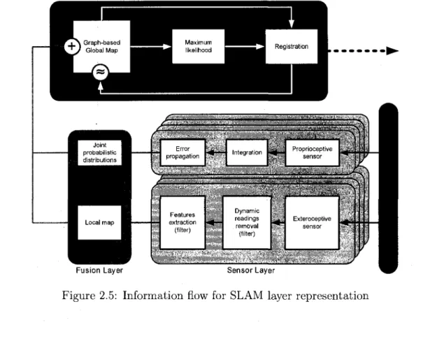
It is possible to separate the sensory layer from SLAM because all exteroceptive and pro-prioceptive sensors end up with the same entry for the SLAM module: a position and an incertitude on this position. In fact, more complex sensing systems such as face tracking [5]'or sound localization [86] outputs can be interpreted as feature poses with their prob-abilistic distributions, exactly as a laser or a sonar sensor do. Adopting such perspective means that the same SLAM algorithm can be used independently of the type of data. Figure 2.5 presents an architecture of a complete SLAM solution based on algorithms sur-veyed in this chapter. It modifies the dashed section presented in the general navigation scheme proposed by Siegwart et al. [76] in Figure 1.1. Sensors are divided in two cat-egories: proprioceptive and exteroceptive. Proprioceptive sensors (e.g., wheel encoders, gyroscopes, accelerometers) for odometry are integrated over time to evaluate the posi-tion. Uncertainties on their readings (represented as a Gaussian with a known variance) are propagated through the integration module which cumulates information over time. This propagation is done using the error propagation law which is explained in Appendix B with an example using differential drive wheel encoders. Each proprioceptive sensor de-rives a possible robot position associated with its covariance matrix which, when combined, are used to find the joint probabilistic distribution of the robot's position. Exteroceptive sensors (e.g., laser, camera, sonar) capture environmental information from which read-ings representing elements moving independently of the robot are detected and filtered out. Additional features (e.g., ViPR, Harris corners, Split-and-Merge, lines, circles, arcs, corners, M-Space) can also be extracted to reduce the amount of data. The results are fused and placed in a spatial data container called local map, using the position estimated with proprioceptive sensors. The local map represents the current perceptual space of the robot. When the incertitude on the position based on odometry is considered too large, a node (i.e., a combination of a position and a local map) is added to a graph-based global map, which is a set of interconnected nodes. This graph representation can be compared to a mass-spring system, as shown in Figure 2.6 (a). A local map is first positioned in the global map based on proprioceptive position evaluation. Then, constraints are derived

based on the estimated relative position of a local map with its surrounding local maps. This constraint evaluation is realized using a registration algorithm. An iterative process called Maximum Likelihood (ML) error relaxation algorithm is applied to readjust local maps positions like in the example of Figure 2.6 (b).

SLAM Layer

Fusion Layer Sensor Layer

Figure 2.5: Information flow for SLAM layer representation

(a) Graph-based global map before relaxation. (b) Graph-based global map after relax-ation.

Figure 2.6: Maximum likelihood error relaxation example.

Although the ML technique is considered the fastest global correction algorithm [38] avail-able, each time a single node is moved, multiple registrations are needed to evaluate new

constraints between nodes. Moreover, if registration is not robust enough in properly eval-uating these constraints (i.e., the position and orientation between two maps), the result of the ML algorithm will lead to an misaligned global map. Registration is therefore a key process in SLAM. Registration must be as fast as possible to avoid computational bottle-neck for real-time performance, and robust to different types of environment to achieve a global map consistent with the real word.

Chapter 3

E X P E R I M E N T A L S E T U P

Our research methodology is divided in two steps: first optimize the ICP algorithm for its use in SLAM for robotics, leading to a new variant that we named Kd-ICP; and then validate the resulting algorithm in simulated and real experimental conditions. Section 3.1 presents the simulated conditions developed to reproduce critical conditions for which the ICP algorithm needs to be optimized in terms of robustness and rapidity. Section 3.2 describes how we proceed with the validation of Kd-ICP in mapping tasks.

3.1 Optimization

To examine the different conditions for which the ICP algorithm needs to be optimized (as described in Chapter 4), we created a test environment to evaluate and analyze the impacts of such optimizations. This test environment is in Matlab1 because of its prototyping and

visualization capabilities. Such simulated test environment provides ground truth data from which it is possible to evaluate the validity of the registration process, in a variety of situations that would be difficult to reproduce in real world settings.

The global map of the test environment was manually developed using GIMP2, a versatile

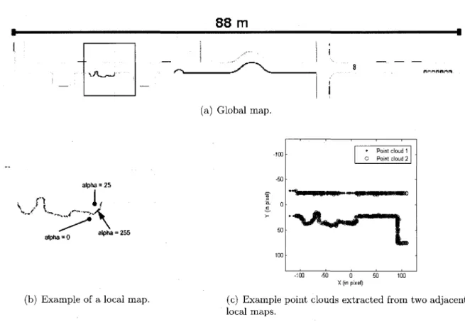
open source graphics manipulation package similar to Photoshop3. Figure 3.1 (a) shows

this environment, which consists of a 88 m long corridor of different shapes (straight, cir-cular), conditions (intersections, doors, corners, obstacles) and colors (expressed in Red, Green, Blue (RGB)). The alpha channel (transparency) is used to simulate occupancy level

1Matlab: h t t p : //www. mathworks. com/

2G I M P : h t t p : //www. gimp. o r g /

obtained from laser range finder readings. Three alpha levels were determined to easily segment the map: 255 represents an obstacle, 25 an explored region without obstacle and 0 an unexplored region. This test environment was then divided into smaller overlapping maps, each map covering an area illustrated by Figure 3.1 (b). Each map represents the perceptual space of a robot being at a specific position in the test environment, moving in the corridor from left to right. These maps are referred to as being local maps. The size of those local maps is fixed based on an hypothesis expressed after conducting pre-liminary trials with a real robot: considering a robot moving in an indoor environment,

a perceptual space with a radius of about 5 meters around the robot discretized uniformly with a resolution of 4 cm is enough to disambiguate two different points of view of this environment. This hypothesis was not directly validated in our work but it appears to

be a good compromise between computation time and precision. The distances between two local maps were randomly distributed between 20 and 60 cm on the x axis with y being constant. The distance used as first guest is 40 cm (i.e., random error is ± 20 cm) is used to simulate odometry information coming from proprioceptive sensors like wheel encoders. A random orientation error of ± 25 degrees is also added to point clouds. Based on those parameters, 176 local maps were used to cover the global map. These local maps are used as ground truth data for registration, because the true position of each local map is known.

To derive sensory readings of a simulated robot with each of these maps, considering that sensor readings are subject to noise, imprecision and occlusion, pixel spreadings and zone deletions were applied to these maps to derive point clouds according to the following parameters:

Sensor noise: a Gaussian additive noise with a standard deviation of 10% of the distance

between the lowest and highest possible value of the RBG channels, and 5% on the alpha channel. Those values were determine empirically. This was realized using the RBG noise filter, a tool available in GIMP. On the RGB channel, this filter simulates possible color variation due to camera errors. Because the alpha channel is used to represents occupancy level, this filter also creates sporadic laser readings that can be caused by very small obstacles like wires.

Sensor imprecision: random pixel spreading with a maximum length of two pixels using

a Spread filter, another tool in GIMP. The Spread filter swaps each pixel with another randomly chosen pixel within the specified range. As an example, after applying the filter to a perfectly straight line, the line has gaps and misaligned pixels while keeping

its main orientation. This filter simulates laser readings with range errors.

Occlusion: a circular zone with a 0.8 meter (i.e., 20 pixels because a pixel represents 4

cm) radius centered randomly is deleted. This data removal reduces the overlapping percentage of two subsequent local maps to simulate occlusion caused by an obstacle near the laser range finder. This occlusion was observed during preliminary trials when the robot passes a doorway or a corridor corner.

The alpha channel is used to extract surface orientation of obstacles since it represents the occupancy level. The surface orientation is represented as a vector perpendicular to the obstacle. A vertical 3 x 3 Sobel filter is applied on the complete alpha channel (representing the occupancy level) to extract the x component of the vector, and a horizontal 3 x 3 Sobel filter is applied for the y component. Because lines have two possible surface orientations, the alpha channel with value greater than zero is used as a mask to cut half of the possibilities. As pointed out in Figure 3.1 (b), this technique can be used because a laser range finder cannot produce readings on the other side of an obstacle. Based on our representation of an occupancy map, pixels on one side of a line representing an obstacle have low alpha values, and pixels on the other side have null values.

This results in having three images of the same size: an image with 4 channels (i.e: RGB and alpha (RGBA)) representing one local map, and two images with a single channel (i.e., gray level) created with the Sobel filtering and representing respectively x and y components of surface orientations. Those images are loaded in Matlab to build a point cloud corresponding to a list of point coordinates with their associate colors and orienta-tions. The length of the orientation vector is calculated for each pixel of the local map. If its length is higher than g, the point is added in the cloud, otherwise it is filtered out. The threshold g was manually adjusted to 30 allowing a good differentiation between obstacles and empty space. Figure 3.1 (c) illustrates one example of two point clouds (blue and red) derived from two adjacent local maps. Simulated sensor noises, sensor imprecision, occlusion and distance between two local maps leading to overlapping point clouds with a small offset can be observed with differences between red and blue point positions.

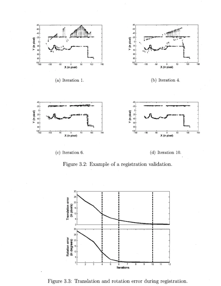
Each time we made a change to the ICP algorithm to derive our Kd-ICP variant, the 176 local maps (or point clouds) were individually registered with the previously one (i.e., point cloud extracted from local map 1 registered with point cloud extracted from local map 2, 2 registered with 3, etc.). As explained in Section 4.1, registration is an iterative process that tries to minimize translation and rotational errors between two point clouds obtained from different perspectives of the same environment. Figure 3.2 illustrates the process with

88 m

ni-irinnr*i«

(a) Global map.

alpha = 25 alpha = 0 alpha = 255 • Point cloud 1 0 Point cloud 2 -" W* -100 -50 0 50 100 X (in pixel)

(c) Example point clouds extracted from two adjacent local maps.

(b) Example of a local map.

Figure 3.1: Test environment for ICP optimization

two point clouds being offset because of an important odometry error. The registration process iteratively tries to minimize these translational and rotational errors in hope of finding a match between the two point clouds. Figure 3.3 illustrates the evolution of the translational and rotational errors in relation to the number of iterations, converging toward zero. Dashed lines represent iterations illustrated in Figure 3.2. We evaluated optimization changes made to the ICP algorithm looking at such curves to make sure that the resulting Kd-ICP variant improves registration performances.

3.2 Validation

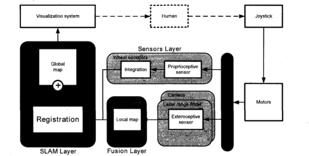
Validation of our Kd-ICP registration algorithm requires to test it in a complete SLAM setup. Figure 3.4 illustrates the block diagram of the system, implemented in C + + . A human operator provides motor command to a robotic platform using a wireless joystick, making the robot safely move in the environment while acquiring three types of sensory readings: laser range finder proximity (i.e., the distance of the nearest obstacle) and

in-f

ifcL •

•150 -100 -50 0 50 100 150

X (in pixel)

(a) Iteration 1. (b) Iteration 4.

X (in pixel)

(c) Iteration 6. (d) Iteration 10.

Figure 3.2: Example of a registration validation.

10 11 12

tensity (i.e., indicating the type of surface reflecting the laser signal) readings, and color readings from the camera, which are representative of the sensors mostly used in SLAM as presented in Section 2.3. These readings are combined to derive 2D point clouds to be processed for registration. In comparison with Figure 2.5, the Error propagation, Dy-namic readings removal and Maximum likelihood modules are not implemented to simplify the implementation while keeping focus on the evaluation of the registration algorithm. Because only one proprioceptive sensor is used, their is no need to fuse information with a Joint probabilistic distributions module either. Registration is done using these point clouds and proprioceptive sensory data coming from wheel encoders (for initial position estimates of point clouds), generating a global map that can be examined using a vi-sualization system [31]. Figure 3.5 presents a snapshot of the interface with Telerobot, a differential drive mobile platform, near a small white refrigerator and a green office separating panel. Telerobot's perceptual space is composed of laser range finder data represented in red and yellow, and an image projection built with video data. This visu-alization system is updated as the robot moves in the environment, showing local maps as they are registered and stored in a global map. The human operator can then validate in real-time the construction of the global map, exploring incomplete regions and react to the information from the robot's perceptual space.

Visualization system

^

^^H ^^H

^ ^ ^ ^ ^ + ^ ^ ^ ^ |

:

•

V

^H|

h

K.

\

J M

CxU'ioct-ptii/e S i - l l V "

>

>

•

lr

•

' '

1

SLAM Layer Fusion Layer

Figure 3.4: Block diagram of the SLAM process implemented for validation of Kd-ICP.

Figure 3.6 illustrates the hierarchical data structure used to store the large amount of data in point clouds. Basically, the environment is represented as a collection of cubic cells in a local map coordinate system, each of them having a position and a set of properties such as occupancy, reflectivity (both derived from the laser) and RGB readings (derived from

Perceptual space

ofTeterobot Globnl map

Figure 3.5: Visualization system used to teleoperate the robot in an unknown environment.

the camera). A property can be represented by a numeric value (between 0 and 255) and a boolean value (true or false) to determine if this specific propriety exist or not for a cell. This boolean value is useful when do not have a color because it is situated outside the field of view of the camera. Wheel encoders and the robot coordinate system are used to specify cells to be updated. For cells that have to combine sensory data over multiple reading cycles, data fusion is done by averaging the readings. This minimizes the impact of dynamic obstacles during the initialization of a point cloud.

Sensory data comes in different coordinate systems which must be linked together. Figure 3.7 shows a simplification in two dimensions of the transformation matrices needed to express sensory data in the global map coordinate system. The transformation matrix

Tgi starts at the origin of the global map and is initialized by the first active local map

created. There is only one active local map at a time, updated with new exteroceptive data at 10 Hz. The robot always moves in the coordinate system of an active local map so

Tir is directly estimated using wheel encoder data. The position of the robot is attached

to the center of its differential drive wheels. Because wheel encoders only give information on x and y translation and on yaw of the robot, the height h of the robot is set to equal the radius of the wheels and is considered constant. This position is assumed to be true for small displacement of the robot. If the robot moves more than a 25 cm radius of the origin of the active local map or if its heading changes more than 10 degrees, a new active local map is created. The position of this new active local map position is set to as product of Tgi by T/r subtracted by h. The matrix Tir is then reset to the origin of the

new active local map with a fixed value of h on the z-axis.

Registration only corrects Tgi and therefore all exteroceptive data must be referred to the

local map. For each obstacle readings returned by the laser range finder, a 4 cm wide cubic cell representing the obstacle is created. From this cell, a ray of empty cells with

Property-occupancy level Local map: 1 Cell: 1 Global map Image Kd-tree Hash table Local-map: 2 Orientation Image Kd-tree Point cloud Hash table

C 3 Z ,

Local map. Local map: n Cell; Cell m Property, red Property blue Property-green Property laser reflectivity

Figure 3.6: Hierarchical data structure used in the validation system.

the same size is assumed between the obstacle and the laser range finder. The difference between an empty cell and a cell representing an obstacle is realized with a property added to a cell called occupancy level. Occupancy level represent the probability of an obstacle at that position with 255 representing 100%. Because the laser range finder error is usually under 4 cm, we fixed the level at 10 (4%) for an empty cell and 255 (100%) for an obstacle. Laser range finder returns also a reflectivity level of the obstacle which is recorded as another property in the cell. The matrix T;r at time t is estimated with

the odometry and Trf representing the position of laser in relation with the center of the

robot is constant because the laser range finder is rigidly fixed to the robot's structure. Thus, all the cells created from the laser range finder and their associated properties at

Global map L°=al map

Figure 3.7: Referential configuration put in place for the validation system.

time t can be expressed in the local map referential using the product of T\r by Trf.

Data from a single camera are radial and do not have depth information like the laser range finder. Moreover, the information from a camera is represented as a rectangular array so a correction based on the lens must be applied. In our system, the correction is directly done in the camera. The transformation matrix Trc can also be determined

because the camera is rigidly fixed to the robot frame. All the obstacle readings coming from the laser can be projected in the camera coordinate system using T~^ times Trf to

retrieve color from the corresponding pixel, which is recorded as three properties (i.e., red, green, blue) [31]. The procedure is slightly modified for cells with low occupancy level: based on the hypothesis that h is constant and knowing the height of the laser range finder with the center of the robot, the position of the floor can be determined; all cells considered as empty are temporarily dropped to the floor level before projecting the color information on those cells and then returned to their original height, as shown in Figure 3.7. The last image is always keep in memory allowing asynchronous color projection each time new laser range finder readings create new cells.

A local map is defined by a position and an orientation (which are initialized using wheel encoder data and modified through registration) and a set of cells, encoded in two spe-cialized data substructures: a hash table and a kd-tree. The hash table associates a key (in our case the 3D position coordinates) to a cell for efficient retrieval and addition when the local map is considered as the active one. We use an open source library of a sparse hash table algorithm4, developed by Google and optimized for speed. This data

struc-ture reduces redundancy in the data. As illustrated in Figure 3.8 (a), cells produced by the laser are radially distributed, which causes a lot of redundant information close to

the laser. In Figure 3.8 (b), cells with the same key added to the hash table are fused together, reducing the number of cells needed to define the same space. When the local map becomes inactive, a point cloud is derived from the hash table by keeping only cells contained in a rectangular prism (empirically set to: height 0.5 m, length 7 m, depth 7 m) around the local map origin. All those filtered cells are reduced to a 2D representation by canceling z coordinates and fusing information of cells with the same x and y coordinates. Note that for our validation setup, we reduce the 3D data to 2D in order to focus our effort on validation of our registration algorithm. To extend the creation of point clouds in 3D, the use of quadtrees and octrees should be examined in order to reduce the number of cells representing empty space and create variable space decomposition like the one shown in Figure 3.8 (c).

(c) Quadtree.

Figure 3.8: Impact of data structures on information reduction.

From the resulting 2D point cloud, all cells with an occupancy level over 200 are used to build a kd-tree optimized to conduct nearest neighbor search. Kd-tree is implemented using the open source Approximate Nearest Neighbor (ANN) library5. After registration,

local maps positions are also encoded in an other hash map associated with the global map and fused together data with identical 2D keys (averaging cell properties and rebuilding a new point cloud). This method makes the local map storing dependent of explored space instead of time, reducing memory requirements of the system. As opposed to our optimization system built in Matlab, the position and orientation of a newly added local map is done by averaging registration results obtained with stored local maps in a radius of 2 m to reduce cumulated errors. To efficiently determine which local maps are close enough to be registered, inactive local map positions are also encoded in a kd-tree associate with the global map.

Finally, an image per local map is created from the 2D cells and sent to the visualization system. Pixels are created based on the position and proprieties of cells. For a cell with an occupancy level higher to 200, the pixel color is a variation of red tone based

5ANN: h t t p : //www. c s . umd. edu/~mount/ANN/

on the reflexivity property. For cells with an occupancy level lower to 200, the pixel color is directly the red, green and blue properties of the cells. The remaining pixel colors corresponding to unexplored area are set to white with an alpha value of zero (full transparency) [31].

Three robotic platforms were used through the validation process, as shown by Figure 3.9. Telerobot is equipped with a rocker-boggie suspension with four omnidirectional wheels. The two motorized wheels have encoders with a resolution of 36,000 ticks per turn and a wheel diameter of 15 cm. The laser range finders used for our trials are the URG range finder, the UTM range finder or the SICK LMS200 with a reading rate of 10 Hz. Their specifications can be found in Table 3.1. The color information comes from a 2.8 mm lens of a Videre STOC-9cm stereo color camera with a frame rate of 7.5 Hz. The image size is 640 x 480 pixels and reduced to 320x240 before compression. We also conducted preliminary trials with a differential drive Pioneer 2 AT robot, equipped with a SICK range finder, and a simulated version of Telerobot using the Player/Stage environment [37]. These setups allowed us to continue working on our project when Telerobot was used in another set of trials or when it was needed for maintenance and recharge.

Stereooamera Passive suspension (a) Telerobot.

o | L

URG range finder

Webcam

Single core, Pentium 1.86 Hz

UTM range finder

Omnidirectional wheels

Sonar

Laser range finder

(b) Pioneer 2 AT. (c) Simulated Telerobot.