OATAO is an open access repository that collects the work of Toulouse
researchers and makes it freely available over the web where possible
Any correspondence concerning this service should be sent
to the repository administrator: [email protected]
This is an author’s version published in: http://oatao.univ-toulouse.fr/23362
To cite this version:
Khemiri, Rihab
and Elbedoui-Maktouf, Khaoula and Grabot,
Bernard
and Belhassen, Zouari Integrating fuzzy TOPSIS and
goal programming for multiple objective integrated
procurement-production planning. (2018) In: Emerging Technologies and
Factory Automation - ETFA 2017, 12 September 2017 - 15
September 2017 (Limassol, Cyprus).
Integrating fuzzy TOPSIS and goal programming for
multiple objective integrated procurement-production
planning
Rihab Khemiri
1, 2, 3, 41
Faculty of Sciences of Tunis University of Tunis El Manar
Tunis, Tunisia
Bernard Grabot
33
LGP-ENIT
INPT- University of Toulouse Tarbes Cedex, France
Khaoula Elbedoui-Maktouf
22
Ecole Nationale d’Ingénieurs de Carthage University of Carthage
Tunis, Tunisia
Belhassen Zouari
44
Mediatron lab, Higher School of Communications of Tunis, University of Carthage
SidiBou Said, Carthage, Tunisia
Abstract—In this paper, a four-phase approach for Integrated Procurement-Production (IPP) tactical planning in a multi-echelon, multi-product and multi-period Supply Chain (SC) network is proposed. To account for ambiguity and vagueness in some real-world data and preferences, in the first phase of the approach, the Fuzzy Technique for Order Preference by Similarity to Ideal Solution (fuzzy TOPSIS) method is used to obtain the overall performance and risk ratings of the suppliers with regard to a set of qualitative and quantitative criteria. In the second phase, we introduce a novel multi-objective possibilistic mixed integer linear programming model (MOPMILP) for solving an IPP planning considering conflicting goals simultaneously: maximization of the overall performance and minimization of the overall risk. Then, after converting this MOPMILP model into an equivalent crisp multi-objective mixed integer linear programming (MOMILP) model, we use the Goal Programming (GP) approach to solve this MOMILP model in order to find an efficient compromise solution (i.e. an efficient procurement production plan) for the whole SC. The proposed approach and solution methodology are validated through a numerical example. Keywords—Integrated Procurement-Production; Fuzzy TOPSIS; performance; risk; Possibilistic mixed integer linear programming; goal programming
I.! INTRODUCTION
Supply Chain Planning (SCP) problem is one of the important issues that face Supply Chain (SC) managers. Traditionally, these problems involve three levels of decision: strategic, tactical and operational. The strategic decisions are related to the SC design, ranging from 5 to 10 years. The major task of the tactical decisions is to determine an optimal use of the various resources on a medium term horizon (from 1 to 2 years). Operational planning decisions search to address an exact scheduling on a short-term horizon (from 1 to 2 weeks). The tactical planning problem is the focus of this study.
Traditionally, production and procurement activities were conducted separately, that may lead to a very poor overall performance [1]. However, in the design of an Integrated Procurement-Production (IPP) system involving resources belonging to different actors within the SC, the decision maker (DM) will be confronted with three important characteristics: (i) Conflicting goals that must be considered simultaneously (e.g., increase performance and at the same time minimize risk). (ii) Presence of different sources of uncertainty such as market demands and available capacities. (iii) Some critical information and preferences are captured through human judgments, and can hardly be expressed using deterministic or probabilistic formulation.
This study suggests to design an IPP planning system for a multi-echelon SC consisting of multiple suppliers, multiple parallel manufacturing plants and multiple subcontractors. To do this, we propose a four-phase approach, which starts with calculating performance and risk ratings of the various actors based on a Multi-Criteria Decision Making (MCDM) approach under a fuzzy environment. In the second phase, the problem is formulated using a Multi-Objective Possibilistic Mixed Integer Linear Programming Model (MOPMILP). Then, in the third phase, an appropriate strategy is applied for converting the MOPMILP into an equivalent crisp Multi-Objective Mixed Integer Linear Programming (MOMILP). Finally, using goal programming (GP) approach, we solve the proposed MOMILP to obtain an efficient compromise solution (i.e. an efficient procurement production plan) for the whole SC.
The rest of the paper is organized as follows. In the next section, we review related works. The proposed four-phase approach is described in section 3. In Section 4, an illustrative example is presented to show the applicability of the proposed
approach. Conclusions and further research directions are discussed in the last section.
II.! LITERATURE REVIEW
In the scientific literature, several models for tactical SC planning under uncertainty are proposed. Most of them are based on stochastic programming models [2], which are generally derived from statistical data. However, in many practical situations, such historical data are often not available and so some imprecise information can, more suitably, be obtained using human subjective judgments. In this case, the Fuzzy Set Theory [3] and the Possibility Theory [4][5] can be used as an efficient way to model uncertainties and subjectivity. Nevertheless, few studies address the IPP planning problem in a fuzzy environment. For example, the authors of [6] propose a multi-echelon, multi-products and multi-periods SC model to deal with the fuzziness of the market demand, the unit costs of raw materials and the unit transportation costs when the objective is to minimize the total cost. A method is also proposed, based on the α-cut representation and Zadeh’s extension principle [4][7] [8], to transform the proposed fuzzy SC model into a family of crisp models. Torabi and Hassini [9] proposed a MOPMILP model for solving an integrated production, procurement and distribution planning problem considering the imprecise nature of some input data as well as two conflicting objective functions: the total value of purchasing and the total cost of logistics. Even if through the first objective, it is proposed to consider the impact of subjective factors in purchasing decisions (such as technical capacities of the suppliers, after sale services and business structure), these criteria are quantitatively evaluated. On the basis of Lai and Hwang’s approach [10][11] and the weighted average method [10][12][13], the original fuzzy model is converted into an equivalent crisp MOMILP model. Finally, a new interactive fuzzy approach is introduced to find a compromise solution. This study was extended in [14] by developing an interactive fuzzy GP approach which incorporates four objective functions: maximizing the total value of purchasing, minimizing the total cost of logistics, minimizing the defective items and minimizing the late deliveries. As in [9], the qualitative factors are quantitatively evaluated. In [15], the authors proposed a fuzzy linear programming based approach to deal with the integrated production, procurement and distribution planning problem. This approach considers the various sources of uncertainty in a SC (process, demand and supply uncertainties) in an integrated manner. The aim of the proposed approach is the best utilization of the available resources so that customer demands are satisfied at minimum cost. Then, the authors introduce a solution procedure for converting the fuzzy model into an equivalent crisp one. This procedure allows the participation of the decision makers, who can express their opinions in linguistic terms. Recently, [16] presented a fuzzy multi-objective mixed-integer nonlinear programming model dealing with a multi-echelon SC. The main objectives of the proposed model are: minimizing the total cost, minimizing the rate of changes of the workforce, improving the customer satisfaction as well as maximizing the total value of purchasing. The fuzzy original model is
transformed into an auxiliary MOMILP model through a three-phase approach. The authors extended then their work in [17] by developing a multi-objective mixed-integer non-linear programming model integrating tactical and operational planning, solved by fuzzy optimization.
We can see that in most of the aforementioned studies, the authors limit their objective to minimize total cost/maximize total profit while satisfying customer demand. In our opinion, these research works fail to address the factors related to risk, which become critical given the rapid market variations. To the best of our knowledge, the only work including a risk management process in an IPP planning model is [18], but this latter does not take into account the lack of knowledge in some critical parameters such as customer demand and partners’ capacities.
Moreover, the survey shows that the majority of existing approaches does not include subjective criteria, or transform them into quantitative ones, as in [9] or [14].
To overcome these limitations, we introduce in this paper an integrated fuzzy!multiple criteria decision making (MCDM) technique and a multi-objective programming approach to deal with an IPP planning system. The MCDM technique is chosen because it is a powerful tool for simultaneously accommodate qualitative and quantitative criteria, whereas using an analytical model is the only way to take into account the various restrictive assumptions of the planning problem.
According to our knowledge, it is the first paper that integrates fuzzy TOPSIS, MOPMILP and GP to solve a multi-echelon, multi-product, multi-period IPP problem including a risk management process. In the next section is summarized the proposed approach.
III.! PROPOSED APPROACH
In this section, we present our four-phase approach dealing with IPP planning, consisting of multiple manufacturing plants, multiple suppliers and multiple subcontractors, considering various sources of uncertainty. We assume that a set of predefined qualified suppliers is provided. The supplier selection problem is indeed not our objective in this work: we focus here on determining the orders to be allocated to each actor (supplier, manufacturing plan and subcontractor). Moreover, since the DM cannot provide exact data for some critical parameters in a mid-term horizon, fuzzy sets and possibility theory is used to handle this vagueness.
In the first phase, the various partners are evaluated using the fuzzy TOPSIS method based on two classes of criteria: performance-based and risk-based decision criteria. In the second phase, the overall performance is computed and the overall risk scores calculated in the first phase serve as input data in the MOPMILP model suggested to determine an optimal procurement-production plan. This possibilistic model is then converted into an equivalent crisp MOMILP using an appropriate strategy. Finally, a multi-echelon, multi-period and multi-product GP method is adopted to solve this MOMILP model and finding a preferred procurement-production plan.
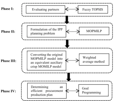
The main steps of the proposed approach are summarized in Fig. 1; more details are given in the following sub-sections. A.! Phase I: Evaluating partners
1)! Selecting decision criteria
Two classes of decision criteria are defined. For each class, we enumerate the most important criteria. The decision maker can select the most appropriate ones according to his strategy.
a)! Class I: Performance-based decision criteria •! Cost: The unit cost related to each partner. •! Capacity: Partners’ production capacity.
•! Quality: The capacity of the partners to deliver the orders with the required quality of packaging. •! Reliability: The ability of the partners to deliver the
orders on time.
b)! Class II: Risk-based decision criteria
•! Flexibility: The ability of the partners to take into consideration the changes in product characteristics proposed by the customer while the order is in process. •! Responsiveness: The ability of the partners to take into
account the changes imposed by the customer in the due dates of orders.
Fig 1. Framework of the proposed approach.
•! Robustness: The insensitivity of the partners to disturbances.
•! Resilience: The ability of the partners to return to a satisfactory state after disruption.
For modelling uncertainty , we assume that the cost and the capacity criteria are given by a triangular fuzzy number, whereas the other criteria are qualitatively assessed by the decision maker using linguistic labels.
2)! Evaluating the performance of each partner
The fuzzy TOPSIS method is used according to the selected Class I criteria for providing an overall rating of each partner. Note that this overall rating, also called the closeness coefficient, is computed according to the distance to both a "negative" (worst) and "positive" (best) ideal solution. Therefore, the ranking of the partners can be determined according to the descending order of the closeness coefficient.
The overall performance rating of a partner j is denoted PIj
3)! Evaluating the risk of each partner
The fuzzy TOPSIS method is also invoked in this step according to the Class II selected criteria. The closeness coefficient related to the partner j is note CCIIj. The overall risk rating of the partner j, equal to 1- CCII j is denoted RIj.
B.! Phase II: Proposed Multi-objective possibilistic mixed integer linear programming model
1)! Formulation of the model a)! Notation
•! Set of indices:
−! T: Set of time periods (t = 1,…,T) −! S: Set of suppliers (s = 1,…, S )
−! M: Set of manufacturing plants (m = 1,…, M ) −! B: Set of subcontractors (b = 1,…, B)
−! R: Set of raw materials (r = 1,…, R) −! P: Set of finished goods (p= 1,…, P)
•! Certain parameters:
−! Sr: Set of qualified suppliers offering raw material r (i.e. Sr ⊆ {1,…,S}).
−! M p: Set of plants producing finished good p (i.e. Mp ⊆ {1,…, M}).
−! Bp: Set of subcontractors producing finished good p (i.e. Bp ⊆ {1,…, B}).
−! αp,r: Quantity of item r to produce a unit of finished good
p.
−! PIj: Performance index for partner j (j∈ {S}U{M_r}U
{M_ov} U {B}) computed using Fuzzy TOPSIS during the first stage, where {M_r} (respectively {M_ov}) represents the set of manufacturing plants producing in regular time (respectively in overtime).
−! RIj: Risk index for the partner j (j∈ {S} U {M_r} U {B})
computed using Fuzzy TOPSIS during the first stage. •! Fuzzy parameters:
−! !"#$%: Demand of final product p in period t.
−! &'()*+$#$% : Production capacity of manufacturing plant m
for product p during period t.
−! &'(),-+$#$% : Overtime capacity of manufacturing plant m for product p during period t.
−! &'()./$#$% : Maximum capacity of
subcontractor b
forproduct p
during period t.
−! &'()0"1$2$%: Maximum procurement capacity of supplier s
for raw material r during period t
.
Phase I:
Phase II:
Phase III:
Phase IV:
Fuzzy TOPSIS
Formulation of the IPP
planning problem MOPMILP
Converting the original MOPMILP model into an equivalent auxiliary crisp MOMILP model
Weighted average method Determining an efficient procurement production plan Evaluating partners Goal Programming
•! Decision variables:
−! x_r m,p,t : Production amount in regular time for product p
at manufacturing plant m in period t.
−! x_ov m,p,t : Production amount in overtime for product p at
manufacturing plant m in period t.
−! x_b b,p,t : Subcontracting amount at subcontractor b for
product p in period t.
−! x_s s,r,t : Purchase amount from supplier s for raw material
r in period t.
−! OV_PI t : Overall performance measurement in period t.
−! OV_RI t : Overall risk measurement in period t.
b)!Objective functions
•! Objective 1: Maximizing the overall performance measurement Max FP= 3456"OV_PI t" " """""""""""""""""""""""""" (1)" Such that: OV_PI t =" 7856" ?":"@A 9":";<" =":"><"( x_s s,r,t * PIs ) + ( x_r m,p,t * PIm_r ) + ( x_ov m,p,t * PIm_ov ) + ( x_b b,p,t * PIb ) Bt (2)
•! Objective 2: Minimizing the overall risk measurement Min FR= 3456"OV_RI t" " """""""""""""""""""""""""" (3)" Such that: OV_RI t =" 7856" ?":"@A 9":";<" =":"><"( x_s s,r,t * RIs ) + (( x_r m,p,t +x_ov m,p,t )* RIm) + ( x_b b,p,t *RIb)""Bt (4) c)!Model constraints C ?":"@A x_r m,p,t +x_ov m,p,t ) + 9":";A" x_b b,p,t D E8$4Bp,t (5) "F)G" H":"IJ s,r,t = ( ?":"@AF_r m,p,t+x_ov m,p,t )* αp,r Bt,Br∈RP (6) x_r m,p,t K LMN)O?$8$4 B m,p,t (7) x_ov m,p,t K LMN)PQ?$8$4 B m,p,t (8) x_s s,r,t K LMN)GH$=$4 B s,r,t (9) x_b b,p,t K LMN)R9$8$4 B b,p,t (10) x_r m,p,t , x_ov m,p,t , x_s s,r,t , x_b b,p,t ≥ 0 Bp, r, t, m, b, s (11)
Constraint (5) ensures the satisfaction of the customers' demand at each period. The amount of raw material to be supplied in each period is determined using constraint (6). Constraints (7) and (8) are respectively the regular and overtime production capacity limitations. Constraints (9) and (10) indicate the limited capacities for each supplier and subcontractor, respectively. Finally, constraint (11) is a non-negativity constraint of the various decision variables.
2)! Model the uncertain input data with triangular possibility distribution
In this study, we adopt the pattern of triangular possibility distribution to represent the uncertain/imprecise data. Fig. 2 shows the triangular possibility distribution of fuzzy number
' = (app, amm, aoo) where app, aoo and amm are the pessimistic, optimistic and most possible value of '.
The imprecise input data for the proposed model can thus be represented using triangular possibility distributions as follows: E8$4 = (E8$4 88 , E8$4??, E8$4SS) B p, t (11) LMN)O?$8$4T"CLMN)O?$8$4 88 ,LMN)O?$8$4?? , LMN)O?$8$4SS ) B"m,p,t (12) LMN)PQ?$8$4TCLMN)PQ?$8$488 ,LMN)PQ?$8$4??,LMN)PQ ?$8$4SS )"Bm,p,t (13) LMN)R9$8$4T"CLMN)R9$8$4 88 ,LMN)R9$8$4??, LMN)R9$8$4SS ) "B"b,p,t (14) LMN)GH$=$4T"CLMN)GH$=$4 88 ,LMN)GH$=$4??, LMN)GH$=$4SS ) """B"s,r,t (15)
C.! Phase III: Strategy for processing the fuzzy constraints Let us consider constraints (5) and (7)-(10) in which the fuzzy left-hand sides are compared to the crisp right-hand sides. A usual method for dealing with such situation is the defuzzification process, which consists in approximating the fuzzy parameters by crisp numbers.
In this work, we use the well-known weighted average method originally proposed in [10] and successfully applied to several problems [9], [12], [13], [14] to convert the fuzzy constraints (5) and (7)-(10).
The popularity of this method is due to its simplicity and its reliability of defuzzification. To do this, we first need to establish the minimum acceptable possibility level of occurrence for the corresponding fuzzy data,"β. Then the equivalent crisp constraints can be stated as follows:
C
?":"@A x_r m,p,t +x_ov m,p,t ) + 9":";A" x_b b,p,t = w1 *"E8$4$U 88
"V w2 *"E8$4$U??"V w3 *"E8$4$USS """ " Bp, t (16)
x_r m,p,t ≤ w1 *"LMN)O?$8$4$U 88
+ w2 *"LMN)O?$8$4$U?? + w3 *"LMN)O?$8$4$USS
Bm,p, t (17) x_ovm,p,t ≤ w1 *"LMN)PQ?$8$4$U 88 + w2 *"LMN)PQ?$8$4$U?? + w3 *"LMN)PQ"?$8$4$USS """"Bm,p, t (18) x_s s,r,t ≤ w1 *"LMN)GH$=$4$U 88 + w2 *"LMN)GH$=$4$U?? + w3 *"LMN)GH$=$4$USS Bs,r, t (19) x_b b,p,t ≤w1*"LMN)R9$8$4$U 88 + w2 *"LMN)R9$8$4$U?? + w3 *"LMN)R9$8$4$USS Bb,p, t (20)
Where, w1 + w2 + w3 = 1 and w1, w2 and w3 represent
respectively the weights of the most pessimistic, the weights of
Fig 2. The triangular possibility distribution of"WX. app amm aoo
the most possible and the weights of the most optimistic value of the fuzzy data. In practice, these weights as well as the minimum acceptable possibility level are determined subjectively based on the DM’s experience.
In this study, we adopt the concept of the most likely values [10], assuming that w1 = w2 = 1/6, w2=4/6 and β = 0.5. The
reason for considering the above weighted values is that the most possible value is frequently the most important one and is associated as a consequence to the higher weight [10].
D.! Phase IV: Goal programming-based solution approach In previous sections, the problem was originally formulated as a MOPMILP model, then converted into an equivalent auxiliary crisp MOMILP model.
Goal Programming (GP) [19] is the most widely used approach to deal with such multi-criteria and multi-objective decision-making problems [20]. GP allows the DM to specify an "aspiration level" for the various goals and to reduce the original problem into a single-objective formulation that seeks to minimize the deviations between the realized results and the aspiration goals. The main advantages of the GP approach are its robustness, its mathematical flexibility and its accuracy, i.e. the possibility to introduce several system constraints [21].
We have used the Weighted Goal Programming (WGP) model to convert the proposed MOMILP model into an equivalent ordinary linear programming model. Consequently, our problem can be reformulated as follow:
Min FGP = wp * YZ[ + wR * Y\] (21) Subject to: (6), (16)-(20) FP"V"^7[T"FP* (22) FR"_"^>[T"FR* (23) Where:
−! FP* is the performance goal calculated using the
mathematical model with objective function (1) subject to constraints (6), (16)-(20).
−! FR* is the risk goal calculated using the mathematical
model with objective function (3) subject to constraints (6), (16)-(20).
−
! ^7[`G"abc"Negative deviation from the target value of performance goal F1*.
−
! ^>] is the Positive deviation from the target value of Risk
goal F2*.
−! d7"and"d> represent respectively the importance weights of the performance goal and the risk goal. These parameters are generally determined by the decision makers such that d7"+ d>= 1.
IV.! NUMERICAL EXAMPLE
To demonstrate the feasibility of the proposed approach, we consider a SC involving three manufacturing plants m1, m2 and m3 and three subcontractors b1, b2 and b3 who provide the finished good p using three common purchased items (one unit
of r1 and two units of r2) which can be supplied from two suppliers (S1 and S2).
The planning horizon is one year decomposed into six monthly periods. These periods correspond to six different forecasted demands with triangular distributions, summarized in Table I. We consider that the DM selects the following criteria:
−! Class I: cost (CI.1), quality (CI.2), reliability (CI.3) and capacity (CI.4).
−! Class II: flexibility (CII.1), reliability (CII.2), resilience (CII.3) and robustness (CII.4).
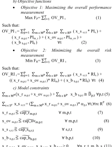
The classical linguistic variables presented in Table II [22] are used to assess the importance weights and ratings of actors. The importance of each decision criteria, as well as the actor’s ratings, are given in Table III – Table VII.
We assume that the DM does not have sufficient information to determine the weights"eZ and e\ of each goal
in the objective function FGP. We thus offer the DM the
possibility of exploring a wider range of potential solutions. To do this, we vary each value of the weights"eZ and e\ between 0 and 1 by increasing one and decreasing the other simultaneously, such that the sum is equal to 1.
TABLEI.FUZZY DEMAND QUANTITIES FOR EACH PERIOD
Periods Demand 1 (110;120;130) 2 (120;135;140) 3 (125;135;145) 4 (145;150;160) 5 (150;160;175)
TABLEII.LINGUISTIC VARIABLES AND FUZZY VALUES [22]
Linguistic Value Very Low (VL) ( 0 ; 0 ; 1 ) Low (L) ( 0 ; 1 ; 3 ) Medium Low (ML) ( 1 ; 3 ; 5 ) Medium (M) ( 3 ; 5 ; 7 ) Medium High (MH) ( 5 ; 7 ; 9 ) High (H) ( 7 ; 9 ; 10 ) Very High (VH) ( 9 ; 10 ; 10 )
TABLEIII.IMPORTANCE WEIGHTS OF CLASS I CRITERIA
Cost Quality Reliability Capacity
VH M ML MH
TABLEIV.IMPORTANCE WEIGHTS OF CLASS II CRITERIA
Flexibility Reliability Resilience Robustness
VH MH ML VL
TABLEV.RATINGS OF THE ACTORS USING SELECTED CRITERIA OF CLASS II
Criteria Actors S1 S2 M1 M2 M3 B1 B2 B3 CII.1 VL M VL MH H VH VH VH CII.2 VL VL L M M MH MH VH CII.3 VL MH VL M MH H VH VH CII.4 VL MH VL VH VH MH VH VH
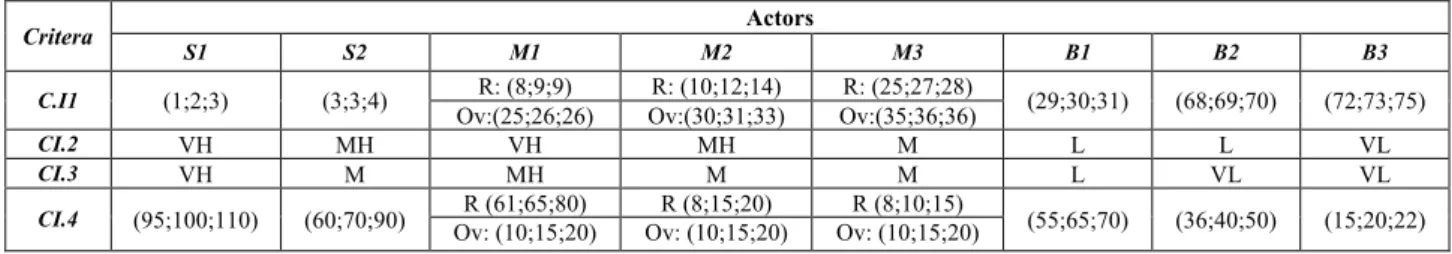
TABLE VI. RATINGS OF THE ACTORS USING SELECTED CRITERIA OF CLASS I
Critera Actors
S1 S2 M1 M2 M3 B1 B2 B3
C.I1 (1;2;3) (3;3;4) R: (8;9;9) R: (10;12;14) R: (25;27;28) (29;30;31) (68;69;70) (72;73;75)
Ov:(25;26;26) Ov:(30;31;33) Ov:(35;36;36)
CI.2 VH MH VH MH M L L VL
CI.3 VH M MH M M L VL VL
CI.4 (95;100;110) (60;70;90) Ov: (10;15;20) R (61;65;80) Ov: (10;15;20) R (8;15;20) Ov: (10;15;20) R (8;10;15) (55;65;70) (36;40;50) (15;20;22)
NB:R: Regular Time; Ov: Overtime
TABLEVII.PERFORMANCE AND RISK MEASURES OF ACTORS
Global indicators
Actors
S1 S2 M1_r M1_ov M2_r M2_ov M3_r M3_ov B1 B2 B3
PI 0.6172 0.4475 0.4090 0.2806 0.2459 0.2300 0.1927 0.1986 0.1992 0.1324 0.0551
RI 0.9437 0.6639 0.9024 0.4901 0.4185 0.3275 0.3212 0.2652
The GP model is solved using the LINGO optimization package. The order quantities assigned to each actor in each period are shown in Table VIII.
Two solutions representing two extreme situations can be identified. In the first one, only objective FP is considered
(eZ=1; e\ =0) and in the second one, only objective FR is
considered. By decreasing by one step the weight of the performance objective and increasing on the other hand the weight of the risk objective, we increase the load of the least risky and least performing actors (i.e. the subcontractors) and we reduce the load of the riskiest and the most performing actors (i.e. the suppliers and the manufacturing plants).
The deviations from the target values for goals FP* and FR*
are summarized in Table IX. The optimum performance measure FP*and the worst risk measure FR* are obtained in the
first extreme situation (eZ=1; e\ =0). In the same way, the
second extreme situation (eZ=0; e\ =1) provides the optimum risk measure FR*and the worst performance measure FP*.
Moreover, by reducing the weight of the performance objective by two steps from its optimal value, we degrade very slightly the performance measure FP and we improve very
slightly the risk measure FR.
Solution (eZ= 0.6; e\ = 0.4) marks a turning point in the evaluation of performance and risk measures. Indeed, the value of the first objective function FP passes abruptly from a
deviation equal to 0.101% to a deviation equal to 84.460% whereas the risk measure is significantly improved (from a deviation equal to 99.648 % to a deviation equal to 13.894%).
For the weights (eZ= 0.5; e\ = 0.5), the performance
measure is slightly degraded (from a deviation equal to 84.460 % to a deviation equal to 99.782 %) and the value of FR
becomes very close to the optimum value FR*.
We also notice that we have obtained very different solutions by varying the weights (eZ; e\). It is then possible to orientate the calculation on a particular solution expressing the compromise required by the DM. However, the compromises achieved are not balanced, given that the performance and risk objectives are not correlated.
V.! CONCLUSION
Nowadays, global SC networks are affected by various sources of uncertainty and imprecision. Consequently, an effective risk management process becomes mandatory for the success of the organization. However, there is still a gap in the scientific literature in providing risk-based factors when designing a SC tactical plan. To deal with this drawback, we present in this paper a four-phase approach integrating Fuzzy MCDM, MOPMILP and GP to deal with a multi-echelon, multi-product and multi-period IPP planning problem under a fuzzy environment.
In the first phase, based on the DM’s judgement and using the fuzzy TOPSIS method, we calculate the overall performance score and the overall risk score of the various partners.
TABLE VIII.PERIODIC ORDER ALLOCATIONS OBTAINED WITH THE GP METHOD
TABLE IX. DEVIATIONS FROM THE TARGET VALUES.
Poids FP FR fg[(%) fh](%) (1,0) (0.9, 0.1) 1660.556 * 2721.815* 00.00 100 (0.8, 0.2) (0.7, 0.3) 1659.267 2714.557 0.101 99.648 (0.6, 0.4) 580.0491 945.9591 84.460 13.894 (0.5, 0.5) 384.0375 659.6424 99.782 0.012 (0.4, 0.6) (0.3, 0.7) (0.2, 0.8) (0.1, 0.9) 383.7282 659.4185 99.80652 0.0012 (0 , 1) 381.2529* 659.3935* 100 00.00
Next, the overall scores of the partners are incorporated into the MOPMILP model in which two important objectives are taken into account: maximizing performance and minimizing risk. In the third phase, the possibilistic programming model is transformed into an equivalent crisp MOMILP model by applying the Lai and Hwang’s approach [10]. Then, a GP approach is applied to determine an efficient compromise solution.
A numerical example is given to demonstrate the importance of the proposed approach.
Future research may focus on the case where several distribution centers are taken into account in the considered SC network to deal with integrated procurement-production-distribution systems.
REFERENCES
[1]! S.K. Goyal and S.G. Deshmukh,“Integrated procurement-production systems: a review,” European Journal of Operational Research, 62(1), pp.1-10, 1992.
[2]! M. Kazemi Zanjani, M. Nourelfath, and D. Ait-Kadi, “A multi-stage stochastic programming approach for production planning with uncertainty in the quality of raw materials and demand,” International Journal of Production Research, 48(16), pp.4701-4723, 2010.
[3]! L.A. Zadeh, “Fuzzy sets”, Information and Control, 8 (3), pp. 338–353, 1965.
[4]! L.A. Zadeh, “Fuzzy sets as a basis for a theory of possibility”, Fuzzy Sets and Systems, 1, pp. 3–28, 1978.
[5]! D. Dubois and H. Prade, Possibility Theory, New York, London, 1988. [6]! S.P. Chen and P.C. Chang, “A mathematical programming approach to
supply chain models with fuzzy parameters,” Engineering Optimization, 38 (6), pp. 647–669, 2006.
[7]! R.R. Yager, “A characterization of the extension principle,” Fuzzy Sets and Systems, 18, pp. 205–217, 1986.
[8]! H.J. Zimmermann, Fuzzy Set Theory and its Applications, 4th Ed, Kluwer-Nijhoff: Boston, MA, 2001.
Poids Periods S1 S2 M1 M2 M3 B1 B2 B3
R1 R2 R1 R2 M1_r M1_ov M2_r M2_ov M3_r M3_ov
(1,0) (0.9,0.1) T1 100 210 21 32 66 15 14 15 1 10 0 0 0 T2 100 210 34 58 66 15 14 15 9 15 0 0 0 T3 100 210 35 60 66 15 14 15 10 15 1 0 0 T4 100 210 35 60 66 15 14 15 10 15 16 0 0 T5 100 210 35 60 66 15 14 15 10 15 26 0 0 T6 100 210 35 60 66 15 14 15 10 15 64 8 0 (0.8,0.2) (0.7,0.3) T1 100 210 21 32 66 1 14 15 10 15 0 0 0 T2 100 210 34 58 66 14 14 15 10 15 0 0 0 T3 100 210 35 60 66 15 14 15 10 15 1 0 0 T4 100 210 35 60 66 15 14 15 10 15 16 0 0 T5 100 210 35 60 66 15 14 15 10 15 26 0 0 T6 100 210 35 60 66 15 14 15 10 15 64 8 0 (0.6,0.4) T1 0 0 39 78 0 0 14 0 10 15 64 17 0 T2 0 0 39 78 0 0 14 0 10 15 64 31 0 T3 0 0 39 78 0 0 14 0 10 15 64 32 0 T4 0 0 46 92 0 0 14 7 10 15 64 41 0 T5 0 0 54 108 0 0 14 15 10 15 64 41 2 T6 13 0 70 166 29 0 14 15 10 15 64 41 19 (0.5,0.5) T1 0 0 0 0 0 0 0 0 0 0 64 41 15 T2 0 0 10 20 0 0 0 0 0 10 64 41 19 T3 0 0 11 22 0 0 0 0 0 11 64 41 19 T4 0 0 27 54 0 0 2 0 10 15 64 41 19 T5 0 0 37 74 0 0 12 0 10 15 64 41 19 T6 13 0 70 166 29 0 14 15 10 15 64 41 19 (0.4,0.6) (0.3,0.7) (0.2,0.8) (0.1,0.9) T1 0 0 0 0 0 0 0 0 0 0 64 37 19 T2 0 0 10 20 0 0 0 0 0 10 64 41 19 T3 0 0 11 22 0 0 0 0 0 11 64 41 19 T4 0 0 27 54 0 0 2 0 10 15 64 41 19 T5 0 0 37 74 0 0 12 0 10 15 64 41 19 T6 13 0 70 166 29 0 14 15 10 15 64 41 19 (0,1) T1 0 0 0 0 0 0 0 0 0 0 61 40 19 T2 0 0 10 20 0 0 0 0 0 10 64 41 19 T3 0 0 11 22 0 0 0 0 10 1 64 41 19 T4 0 0 27 54 0 0 2 0 10 15 64 41 19 T5 0 0 37 74 0 0 12 0 10 15 64 41 19 T6 13 0 70 166 29 0 14 15 10 15 64 41 19
[9]! S.A. Torabi and E. Hassini, “An interactive possibilistic programming approach for multiple objective supply chain master planning,” Fuzzy Sets and Systems, 159 (2), pp. 193–214, 2008.
[10]! Y.J. Lai and C.L. Hwang, “A new approach to some possibilistic linear programming problems,” Fuzzy Sets and Systems, 49, pp.121–133, 1992. [11]! Y.J. Lai and C.L. Hwang, Fuzzy Multiple Objective Decision Making,
Methods and Applications, Springer, Berlin, 1994.
[12]! T.F. Liang, “Distribution planning decisions using interactive fuzzy multi-objective linear programming,” Fuzzy Sets and Systems, 157, pp.1303–1316, 2006.
[13]! R.C. Wang and T.F. Liang, “Applying possibilistic linear programming to aggregate production planning”, International Journal of Production Economics, 98, pp. 328–341, 2005.
[14]! S.A. Torabi and E. Hassini, “Multi-site production planning integrating procurement and distribution plans in multi-echelon supply chains: an interactive fuzzy goal programming approach”, International Journal of Production Research, 47 (9), pp. 5475-5499, 2009.
[15]! D. Peidro, J. Mula, M. Jiménez and M. del Mar Botella, “A fuzzy linear programming based approach for tactical supply chain planning in an uncertainty environment”, European Journal of Operational Research,205(1), pp. 65-80, 2010.
[16]! N. Gholamian, I. Mahdavi, R. Tavakkoli-Moghaddam and N. Mahdavi-Amiri, “Comprehensive fuzzy multi-objective multi-product multi-site aggregate production planning decisions in a supply chain under uncertainty”, Applied Soft Computing, 37, pp. 585-607, 2015.
[17]! N. Gholamian, I. Mahdavi and R. Tavakkoli-Moghaddam, “Multi-objective multi-product multi-site aggregate production planning in a supply chain under uncertainty: fuzzy multi-objective optimisation”, International Journal of Computer Integrated Manufacturing, 29 (2), pp. 149-165, 2016.
[18]! R.Khemiri, K. Elbedoui-Maktouf, B.Grabot and B.Zouari, “A fuzzy multi-criteria decision making approach for managing performance and risk in integrated procurement-production planning,” International Journal of Production Research, in press.
[19]! A. Charnes and W.W.Cooper, Management models and industrial applications of linear programming, New York: Wiley,1961.
[20]!C. T. Chang, “Binary fuzzy goal programming”, European Journal of Operational Research, 180(1), pp. 29-37, 2007.
[21]! I. Dhahri and H. Chabchoub, “Nonlinear goal programming models quantifying the bullwhip effect in supply chain based on ARIMA parameters,” European Journal of Operational Research, 177(3), pp. 1800-1810, 2007.
[22]! S. H. Amin and J. Razmi, “An integrated fuzzy model for supplier management: A case study of ISP selection and evaluation”, Expert systems with applications, 36(4), pp. 8639-8648, 2009.
![TABLE II. L INGUISTIC VARIABLES AND FUZZY VALUES [22]](https://thumb-eu.123doks.com/thumbv2/123doknet/2994755.83944/6.892.470.827.640.787/table-ii-l-inguistic-variables-and-fuzzy-values.webp)