Any correspondence concerning this service should be sent
to the repository administrator:
[email protected]
This is an author’s version published in:
http://oatao.univ-toulouse.fr/22534
Official URL
DOI :
https://doi.org/10.1109/SASO.2018.00018
Open Archive Toulouse Archive Ouverte
OATAO is an open access repository that collects the work of Toulouse
researchers and makes it freely available over the web where possible
To cite this version:
Verstaevel, Nicolas and Georgé, Jean-Pierre and
Bernon, Carole and Gleizes, Marie-Pierre A Self-Organized Learning
Model for Anomalies Detection: Application to Elderly People. (2019)
In: 12th IEEE International Conference on Adaptive and
Self-Organizing Systems (SASO 2018), 3 September 2018 - 7 September
2018 (Trento, Italy).
A
Self-Organized Learning Model for Anomalies
Detection:
Application to Elderly People
Nicolas Verstaevel
SMART Infrastructure Facility University of Wollongong Wollongong, Australia [email protected] Jean-Pierre Georg´e IRIT Universit´e de Toulouse Toulouse, France [email protected] Carole Bernon IRIT Universit´e de Toulouse Toulouse, France [email protected] Marie-Pierre Gleizes IRIT Universit´e de Toulouse Toulouse, France [email protected]
Abstract—In a context of a rapidly growing population of elderly people, this paper introduces a novel method for be-havioural anomaly detection relying on a self-organized learning process. This method first models the Circadian Activity Rhythm of a set of sensors and compares it to a nominal profile to determine variations in patients’ activities. The anomalies are detected by a multi-agent system as a linear relation of those variations, weighted by influence parameters. The problem of adaptation to a particular patient then becomes the problem of learning the adequate influence parameters. Those influence parameters are self-adjusted, using feedback provided at any time by the medical staff. This approach is evaluated on a synthetic environment and results show both the capacity to effectively learn influence parameters and the resilience of this system to parameter size. Details on the ongoing real-world experimentation are provided.
Index Terms—Multi-agent systems, Anomaly detection, Smart health
I. INTRODUCTION
Clinical observations have proven that human’s biological functions (such as temperature, weight or arterial pressure) follow periodical variations regulated by the internal biolog-ical rhythm [1]. Human’s daily activities also have periodi-cal rhythms due to biologiperiodi-cal imperatives (sleeping, eating, drinking...), environmental conditions (days and nights cycles, season cycles), and social components (agenda, education, culture, sports...) [2]. Human’s daily activities and biological rhythms are thus intrinsically correlated, and monitoring the Circadian Activity Rhythm1 of an individual provides useful
information that may be used in a medical follow-up. This biological tendency for humans to have some regularities in their everyday life enables to model everyday life behavioural rhythms in order to study deviation and anomalies [3] [2].
The will to detect anomalies in elderly people’s behaviour arises with the evolution of IoTs and Smart Homes which now enables to equip houses with sensors, effectively monitoring different aspects of everyday life [4]. Behavioural anomaly 1A Circadian Activity Rhythm is a daily rhythmic activity cycle, based
on 24-hour intervals, that is exhibited by many biological organisms such as humans
detection is an active science field covering the different aspects of Telecare and Telehealth [5] [6] [7]. The major difficulty in this work is that the notion of anomaly is difficult to clearly specify as it is highly related to patient habits and pathology types/progression, and that is why artificial intelligence and particularly machine learning techniques have been used to learn to detect those anomalies. Those approaches might be classified into three categories [8]:
• Supervised anomaly detection techniques which produce
classifiers using labelled examples of normal and anoma-lous situations, and then label new situations as normal or anomalous.
• Semi-supervised anomaly detection techniques that build
a model of the normal behaviour from given examples of normal behaviour and then evaluate the likelihood of new instances with the learnt model.
• Unsupervised anomaly detection techniques that detect
anomalies in unlabeled dataset under the assumption that the majority of instances in the dataset are normal. All those approaches require to collect data prior to the detec-tion, either to label them or to tune the anomaly detection algo-rithm. Traditionally, anomaly detection approaches in elderly people are based on pre-established models, modeling either the elderly activity or the disease to monitor. For example, [9] monitors daily living activities to evaluates dependency based on geriatric scales. This offline gathering of data reduces the capacity of adaptation of those algorithms to variations that may occur in patient’s everyday life or in his pathology.
In this paper, we propose a novel approach based on a multi-agent system to detect in real-time behavioural anomalies by using feedback from the medical staff. The usage of the multi-agent paradigm has shown interesting results in e-health as it naturally fits with the ambient assisted living paradigm, composed of many heterogeneous and distributed devices in a highly dynamical environment in strong interaction with humans [10] [11] [12] [13]. The novelty of our approach is that it transforms medical staff feedback into constraints and thus, approaches the problem of adaptation of the anomaly
detection algorithm to a patient and his pathology through a real-time linear optimization process. The rest of the paper is organized as follows: Firstly, section 2 introduces a model for anomaly detection through sensor events, then the multi-agent system designed to learn weights in real time is described in section 3, and finally, before concluding, section 4 presents experiments showing the capacity of the multi-agent system to effectively learn the weight parameters.
II. A MODEL FORANOMALYDETECTION THROUGH
SENSOREVENTS
This section presents a new model for anomaly detection. We present this model in the context of monitoring elder’s habits from the observation of the Circadian Activity Rhythm of a patient through sensors events with a medical follow-up. The model is composed of three components: the observa-tion of variaobserva-tions in the behavioural rhythm of a patient, the modelling of a pathology to monitor through a linear relation between the observed variations, and the transformation of feedback from the medical staff into constraints. The rest of this section is organized as follows. First, we define the activation profile of a sensor and its nominal profile, which are used to compute a disparity value to detect variations in sensors activation. Then, we introduce the problematic of anomaly detection and its adaptation to both the patient and his pathology through a linear relation. Finally, we present how feedback from medical staff are used to transform the problem of adaptation of the anomaly detection to a patient and his pathology into a dynamic constraint solving process, and discuss the genericity and novelty of this model.
A. Activation Profile
The environment of the patient is observed through a set of sensors S, where each sensor s ∈ S monitors a particular activity2. Those sensors provide discrete (such as the presence in a room or the opening of a door) or continuous data (such as pressure or temperature sensors). The daily activity of a patient is split into N slices of equal duration in order to build a Circadian Activity Rhythm.
The change of value of a sensor s ∈ S produces an event et
s∈ R associated with the sensor s at the time t ∈ [0, N ]. The
value of et
s is either 0 (for deactivation) or 1 (for activation)
for discrete sensors, and a real value for continuous sensors. A setAt
s ofN events describes the activation profile of a
sensor during the last N cycles. At s= [e 1 s, e 2 s, ..., eNs ] (1)
At each time stept, we have for each sensor an activation profile describing the effective Circadian Activity Rhythm of the user.
2Table I summarizes all notations and formulas.
B. Nominal Profile
In order to detect anomalies and drifts, the activation profile of a sensor must be compared with a reference profile that models the regularities of behaviour of the user. To model those regularities of behaviour, we introduce the nominal profile of a sensor.
Pt
s is the set of reference values that defines the nominal
profile at the timet of the sensor s ∈ S where rt
s∈ IR is the
reference value of the sensors at time t ∈ [1, N ]: Pt s = [r 1 s, r 2 s, ..., rsN] (3)
Therefore, a reference value is associated with each slice of a day. There are many ways to build such reference values. For instance, we can use a simple λ function to compute and update the nominal profile. At any new event ei
s, the
valueri∗
s of a reference valuerisis updated using the formula:
ri∗
s = rsi· λ + eis· (1 − λ) (2)
whereλ ∈ [0, 1] is a parameter that enables to determine the importance of the new slice over the old one. The easiest way to build such a value is to compute the mean value between the reference value and the event value leading to a λ value of0.5.
As the focus of this paper is anomaly detection and not behavioural modelling, we take the assumption that we do dispose of a set of nominal profiles and reference values, no matter how those references values have been computed. This hypothesis is discussed in section II-H and section V provides details on a real-world experimentation.
C. Disparity Values
Now considering that at each time step t, we have at disposal both an activation profile and a nominal profile for each sensor s, we can express the dissimilarity of the two profiles∆t
s within the last 24 hours by computing:
∆t s= N P i=1 |ri s− eis| (4)
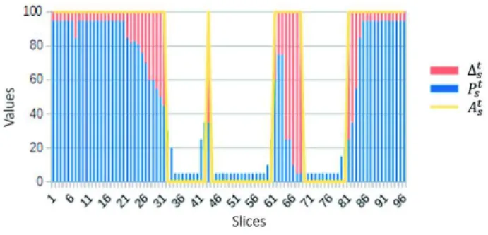
This corresponds to the sum of absolute values of the differences between the activation profile and the nominal profile within the last 24 hours. Figure 1 illustrates, Pt
s, Ats
and∆t
s for a specific sensor s.
D. Anomaly Detection
Anomaly detection consists in rising alerts when a deviant behaviour is detected. The disparity value introduced in the previous section enables to detect variations in the behavioural rhythm of the patient over the last 24 hours. However, a disparity value higher than 0 is not necessarily an anomaly as there may be some variability in a patient’s behaviour. For instance, waking up a little bit earlier than usual should not trigger the alert process. Furthermore, anomalies may rise from a combination of events such as no one is in the bedroom at 9pm and the main door is open. To take this into
Figure 1. The disparity ∆t
s is calculated from the difference between the
activation profile At
sand the nominal profile Pstof a sensor s at time t over
the last 24 hours
account, we propose to detect anomalies through a linear combination3 of the disparity values ∆t
s of each sensor s.
To model the influence of each dissimilarity value in the anomaly, we introduce a weight value ωs ∈ IR associated
with each sensor s. The degree of anomaly of a situation Dt
is computed at each time stept: Dt= P
s∈S
∆t
s· ωts (5)
Anomaly detection then consists in rising an alert whenever the degree of anomaly of a situation reaches a certain threshold T ∈ IR:
Dt> T (6)
The value of T and the weight parameters ωt
s have to be
chosen accordingly to the patient in order to provide person-alized anomaly detection. In the next section, we propose to perform this adaptation by using feedback from the medical staff.
E. Personalized Adaptation to a Patient
In order to adapt the model to a given patient, two compo-nents have to be taken into account: the behavioural rhythm of the patient, and the pathology to monitor. The first component, the behavioural rhythm, is modelled through the nominal profiles of sensors. The second component, the pathology to monitor, is modelled through the weights associated with the sensors for computing the degree of anomaly of a situation.
Thus, adapting the model to a patient results in solving those two questions:
• How to adapt in real-time the nominal profile in order to
fit with the behavioural rhythm of the patient and have an up-to-date profile that can be used to detect variation in its behaviour?
3We chose a simple linear combination because the idea is that the relevance
of the system does not come from the model produced by the learning algorithm at a specific time, but from the constant and on run-time adjustment this algorithm is able to do.
• How to tune the weights of the anomaly detection in order
to adjust the anomaly detection to the pathology of the patient?
Those two questions involve to approximate the optimal parameters P∗
s and ω ∗
s for each sensor s that perform an
optimal detection of anomalies fitting with both the patient behavioural rhythm and pathology. In the rest of this paper, we focus on the second question, while the first question is already addressed by the model in section II-B with the update of the nominal profile.
F. Feedback Constraints
Whenever an alert is triggered, the information is sent to the medical staff which can provide feedback on the quality of the alert (false positive, false negative, true positive or true negative). This feedback enables to express constraints about the degree of anomaly of the situation and the current values of the weightsωt
s:
• False positive: the system has triggered an alert whereas
no abnormal behaviour was detected by the medical staff. The situation t which degree of anomaly has led to raise an alert should have not exceeded the threshold and thus the degree of anomaly of the situation should be lower.
P
s∈S
∆t
s∗ ωts≤ T (7)
• False negative: the medical staff has detected an
anomaly in a period P whereas no alert was triggered by the system. If the medical staff cannot point out the timet where the anomaly should have been raised, there should have been at least one degree of anomaly over the considered period that has exceeded the threshold value.
∃t ∈ P,P
s∈S
∆t
s∗ ωts> T (8)
If the medical staff can point out exactly the time t where the anomaly should have been raised, the formula becomes:
P
s∈S
∆t
s∗ ωts> T (9)
• True positive: the system has raised an alert and the
medical staff confirms this abnormal situation. The degree of anomaly of the situation t should always exceed the threshold.
P
s∈S
∆t
s∗ ωts> T (10)
• True negative: the system has raised no alert and the
medical staff confirms that there was no anomalous situation. The degree of anomaly of the situation t should never exceed the threshold.
P
s∈S
∆t
s∗ ωst≤ T (11)
Each feedback enables to generate a set of inequalities pro-viding useful information on the nature of the optimal weights ω∗
s. Dynamically solving those inequalities by adjusting the
current weights ωt
s acts as an heuristic guiding the tuning of
the weights and thus, fitting the anomaly detection system with the patient and his pathology. Thus, the process of anomaly detection then becomes a process of linear optimization with a dynamic set of constraints. It should be noted that with this method, the effective value of the threshold T is not a parameter to adjust, but a fixed parameter that could be chosen arbitrarily, as the weights will adapt to this threshold during the solving process.
G. Synthesis of the Model
Table I presents a table that sums-up the model for anomaly detection and the different parameters. The model proposes to build and update a nominal profile of the Circadian Activity Rhythm of a set of sensors describing the patient’s habits and to compute the disparity between this nominal profile and the activation profile of the sensor. This disparity is used to com-pute the degree of anomaly of the current situation, weighted by the weight of each sensor. Whenever the degree of anomaly reaches a threshold T , an alert is triggered. The problem of fitting this model with a patient then results in finding the adequate weights for the sensors to raise only positive alerts. Feedback of false positive, false negative, true positive and true negative sent by the medical staff enables to dynamically build inequalities providing information about the values of those weights. Solving dynamically those inequalities by adjusting the weights of the sensors will allow the system to converge in order to detect the desired anomalies.
H. Novelty and Genericity
The problematic of anomaly detection is studied within di-verse research areas and application domains [14]. Compared to existing approaches in scientific literature, the novelty of our model lies in the transformation of the initial problem of anomalies detection into a problem of constraint solving. Furthermore, our proposal to detect anomalies through a linear combination of various values and not to build the detection on any prior hypothesis on the nature of those values or their dynamic, enables this model to be re-used in any problem in which a set of values expressing a distance between an observed behavior and an expected one have to be used to characterize a situation. The only adaptation of our model required for changing the domain is the Nominal profiles of sensors used to compute the disparity values. However, as illustrated in the rest of this paper, those nominal profiles do not interfere with the self-organized learning process. The next section, which describes the core of the self-organized learning process and addresses the problematic of adjusting in real-time the weightsωt
s to satisfy a dynamic set of constraints, is thus
domain agnostic.
III. A MASFORREAL-TIMEDETECTION OF
BEHAVIOURALANOMALIES
[15] proposes to address complex systems with a bottom-up approach where the concept of cooperation acts as the core of self-organization. According to [16], the design of a cooperative entity could be described by a nominal behaviour, which corresponds to the behaviour that the entity has when the system is in a functional state, and a cooperative behaviour, which is a subsumption of the nominal behaviour consisting of a set of rules that are triggered to repair the adequacy of the system.
The rest of this section is organized as follows: a description of the functionality of the system and its environment are provided. Then, the agents and their nominal behaviours are presented. In the last part, the cooperative rules that enable the system to anticipate or repair failures in these nominal behaviours are introduced, enabling to solve the initial problem of weights adjustment (see section II-E).
A. Functionality of the System
In section II, we introduced a model for anomaly detection from a flow of events coming from sensors. This model detects anomalies through a linear combination of the variations be-tween an activation profile and a nominal profile. In response, the medical staff can send qualitative feedback about those alerts. We introduced that adapting this model to a patient consists in approximating the weightωs associated with each
sensor in accordance with the constraints that are raised by the medical staff. The functionality of the multi-agent system is then to monitor events coming from sensors and to compute the degree of anomaly of the situation that is sent to the trigger alert rule in order that only true positive alerts are raised.
B. Environment
From the model description are identified three different entities that the system has to interact with:
• Sensors that are active entities that send events to the
system.
• The alert rule that is a passive entity that receives the
degree of anomaly of a situation and triggers or not an alert.
• The medical staff that is an active entity that sends
feedback on false positive, false negative, true positive and true negative alerts.
Those three entities compose the environment of the MAS. The MAS has to gather information from sensors and the medical staff has to provide the alert rule with an adequate degree of anomaly about the current situation.
C. Agents
Three types of agents compose the MAS: Profile agents, Weight agents and Constraint agents. In this section, each agent and its nominal behaviour, describing the normal be-haviour that the agent should follow, are introduced. Then, cooperative rules are added to resolve or anticipate failures that may happen in the nominal behaviour of an agent. Learning and adaptation are the result of those cooperative rules.
Parameter Description
s∈ S A sensor s belonging to the set of sensors S.
N Unit time (Number of equal time slices that split a day). t The current time corresponding to a particular time slice. et
s∈ IR An event that occurred on the sensor s at time t.
At
s= [e1s, e2s, ..., eNs ] The activation profile of a sensor s at time t composed of a set of N events.
rt∈ IR A reference value describing an expected event at a time t.
Pt
s = [r1s, rs2, ..., rNs ] The nominal profile of a sensor s at time t composed of a set of N reference values.
∆t s= N P i=1 |ri
s− eis| The disparity between the activation profile Ats and the nominal profile Pst of the sensor s at time t.
ωs∈ IR The weight associated with the sensor s.
Dt= P s∈S
∆t
s· ωts The degree of anomaly of the situation t computed from the disparity value and weight of each sensor.
Dt> T The alert triggering rule with T ∈ IR.
P
s∈S
∆t
s· ωts≤ T Inequalities raised by a false positive feedback or a true negative feedback at time t.
P
s∈S
∆t
s· ωts> T Inequalities raised by a false negative feedback or a true positive feedback at time t.
Table I
SYNTHESIS OF THE MODEL AND PARAMETERS
1) Nominal Behaviours:
a) Profile agents: A Profile agent is associated with a specific sensors of the environment and with a unique Weight agent. It models the nominal profile and activation profile of a sensor (see section II-A and II-B). Its function is to compare the activation profile of a sensor to its nominal profile and send the disparity value to its associated Weight agent. The nominal behaviour of this agent is described by the algorithm 1.
b) Weight agents: A Weight agent is associated with a unique Profile agent and interacts with all Constraint agents. It corresponds to the valueωs of the model (see section II-F).
The role of a Weight agent is to dynamically compute and send the value∆t
s· ωs to the alert rule. In this nominal behaviour,
all constraints are satisfied and no update is necessary. The nominal behaviour of a Weight agent is described by the algorithm 2. The nominal behaviour of a Weight agent does not include the weight adjustment rules. This behaviour will be introduced in its cooperative behaviour (see section III-C2c).
c) Constraint agents: A Constraint agent models an in-equality and computes a criticality which expresses its degree of satisfaction. A positive criticality means that the constraint is violated, a criticality negative or equal to zero means that the constraint is satisfied. Thus, the local objective of each Constraint agent is to minimize its criticality. When the system is in a nominal behaviour, each Constraint agent is satisfied. The nominal behaviour of a Constraint agent is described by the algorithm 3.
Algorithm 1 Nominal behaviour of a Profile agent associated with a sensors.
Require: An eventet
s, a nominal profilePst
1: Update the activation profileAt
s fromAt−1s to includeets
2: Compute the dissimilarity value∆t s
3: Send∆t
s to the associated Weight agent
Algorithm 2 Nominal behaviour of a Weight agent. Require: ∆t
s from its associated Profile agent.
1: Compute and send the value∆t
s·ωsto its associated Profile
agent
Algorithm 3 Nominal behaviour of a Constraint agent.
1: Update the criticality of the agent using the formula (P
s∈S
∆t
s·ωs−T )·relation where T is the threshold value
of the inequality andrelation is the sign of the relation (1 if the relation is > and −1 if the relation is ≤)
d) Synthesis: Figure 2 synthesizes the nominal behaviour of the MAS system. A set of sensors sends events to a set of Profile agents. Those Profile agents model both the activation profile and the nominal profile of a sensor. Each Profile agent computes its disparity value∆s and sends it to its associated
Weight agent. Then, each Weight agent computes the value ∆s· ωs and sends it to the alert rule. At last, the alert rule
sums all the values sent by Weight agents and compares it to the thresholdT to rise or not an alert. This nominal behaviour corresponds to the system’s normal behaviour, i.e. when the
system has managed to adjust weights in compliance with the constraints to raise only true positive alerts. By itself, the nominal behaviour is not able to learn. Learning and adaptation are enabled by the cooperative rules.
2) Cooperative rules: The cooperative behaviour of an entity describes a set of rules that allows the entity to achieve its nominal behaviour by either anticipating or repairing failures. From the description of the nominal behaviour of the MAS, a failure of the system results in raising false positive or false negative alerts that are detected with the feedback from the medical staff. Those failures come from a wrong estimation of the weights ωs by the Weight agents
which led to a wrong collective estimation of the criticality Dt of a situation. The cooperative rules should then enable
the Weight agents to adjust their weights in order to reach back a nominal behaviour. This adjustment involves active cooperative interactions with the Constraint agents.
In the rest of this section, we describe the cooperative process that leads to the adjustment of the weights by the Weight agents. This process involves four activities: the dy-namic creation of Constraint agents to model feedback from the medical staff, the request sent by Constraint agents to the Weight agents, the Weight agents self-tuning of their value, and the quickening of the Weight agents self-tuning. Those activities are added to the nominal behaviour. The rest of this section describes each of these activities.
a) Creation of Constraint agents: Constraint agents model the inequalities expressed by the feedback from the medical staff. Initially, the system possesses no Constraint agent. A new Constraint agent is created whenever a feedback is received by the system to model the inequality associated with the feedback according to Table II. When created, a Constraint agent stores the ∆t
s values associated with the
medical feedback. Those values are fixed at the agent creation, and are the ones that the agent will always use to compute its own criticality with the current weights of the Weight agents using the formula described in section III-C1b. Each Constraint agent aims to be satisfied, by having a criticality lower than zero. Therefore, a Constraint agent can be seen as a solicitor agent: it requires a service, the minimizing of his criticality, that can only be provided by the Weight agents.
b) Interaction between Constraint agents and Weight agents: At each time step, Constraint agents compute their criticality and send personalized requests towards each Weight agent involved in their inequality providing information about the service needed by the Constraints agents. This request contains three pieces of information: the current criticality
Feedback Constraint Agent Creation Inequality
False positive Dt≤ T
False negative Dt> T
True positive Dt> T
True negative Dt≤ T
Table II
TYPE OFCONSTRAINT AGENT INEQUALITY ACCORDING TO THE TYPE OF REQUEST.
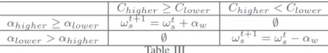
Chigher≥ Clower Chigher< Clower
αhigher≥ αlower ωt+1s = ωts+ αw ∅
αlower> αhigher ∅ ωt+1s = ωts− αw
Table III
THE COOPERATIVE DECISION OF AWEIGHTAGENT.
of the Constraint agent, the desired direction of variation (relation > or ≤), and the influence αw of the Weight agent
w in the inequality. This latter influence is computed with the disparity values ∆c
s that were memorized by the Constraint
agentc at its creation using the following formula: αw= |ωw· ∆cw|/
P
s∈S
|∆c
s· ωs| (12)
c) Weight agents self-tuning: At each time step, a Weight agent receives feedback from Constraint agents. The agent identifies Chigher and Clower which are respectively the
Constraint agent requesting an increase (relation >) with the higher criticality level and the Constraint agent request-ing a decrease (relation ≤) with the higher criticality level. As Chigher and Clower are the most constrained Constraint
agents, reducing the criticality of Chigher will also reduce
the criticality of every other Constraint agent requesting an increase. Reciprocally, reducing the criticality ofClower will
also reduce the criticality of every other Constraint agent requesting a decrease. However, asChigherandClowerrequest
antagonist actions, reducing the criticality of one involves to increase the criticality of the other. Every agent must locally choose the most cooperative action, which involves to reduce the difference between the criticality of Chigher and Clower.
Indeed, by helping one of the Constraint agents, the Weight agent should not make the criticality of the latter exceeds the former. The agent decision is based on its influencesαhigher
and αlower that express its contribution to each of the two
constraints. Depending on which of the two Constraint agents has the higher criticality and the influences of the Weight agent on these two constraints, the Weight agent can decide to do nothing or to increase or decrease its current value according to Table III. The value of the decrease or increase is the influence of the most critical Constraint agent. The Weight agent always decides to perform the action that is expected to have the most cooperative impact on the system, which means reducing the maximum criticality ofChigher andClower.
d) Quickening the search: Since the value of adjustment made by the Weight agents is based on their influence, the adjustment step is bounded to a maximum of1, as α ∈ [0, 1]. It might lead to situations where equal successive adjustments are required to reach a certain value. Reciprocally, it might prevent the system to reach a certain level of precision as the influence might be higher than the required precision. In order to increase or reduce the adjustment step of the weight, we introduce a parameter β specific to each agent into the weight adjustment formulas:
ωt+1
ωt+1
s = ωts− β · αw in the case of a decrease (14)
The adjustment of this β parameter is based on adaptive value trackers, a tool introduced by [17] which can be seen as an adaptation of dichotomous search for dynamic values. The β parameter is increased by 2 when two successive actions are performed (either two successive increases or decreases), and decreased by 1/3 when two different actions are performed (either an increase followed by a decrease, or a decrease followed by an increase). Situations where the Weight agent decides to perform no action are not considered by the β adjustment. The adaptive adjustment of the β value behaves either as a stimulant or an inhibitor of the weight adjustment, facilitating the search of weight values.
The number of Constraint agents is limited to 2n where n is the number of Weight agents. Whenever the number of Constraint agents has reached this limit, the creation of a new Constraint agent leads to the removal of the Constraint agent with the same relation (> or ≤) having the lowest criticality value. This allows to keep the most recent and constrained Constraint agents. Another aspect of this limit is that, as the number of Constraint agents is limited, the complexity of a decision cycle is then bounded.
e) Synthesis: The cooperative rules described in this sec-tion enable each Weight agent to tune its weight in accordance with the Constraint agents that are dynamically created. The resolution process is then a succession of feedback coming from Constraint agents and decisions from the Weight agents based on the criticality of the most constrained Constraint agents and the influence of the Weight agents on these constraints. The successive resolution of inequalities enables the Weight agents to tune their weights, and thus to converge towards optimal parameters. The overall algorithm is described in algorithm 4. The complexity of one resolution cycle of this algorithm is of the order of O(CW ), with C the number of Constraint agents andW the number of Weight agents.
Algorithm 4 MAS lifecycle
1: loop
2: if Medical staff feedback received then
3: Create a new Constraint agent to model the received feedback
4: end if
5: if New events occurred then
6: Each Profile agent updates and sends disparity values ∆t
s to the Weight agents
7: end if
8: Update Constraint agents criticality
9: Send Constraint agents feedback to Weight agents
10: Do the decision for each Weight agent
11: Each Weight agent computes and sends the value∆t s·ωst
12: Test the alert rule
13: end loop
IV. EXPERIMENTS AND RESULTS
In order to study the ability of the proposed MAS to dy-namically adjust its weights in accordance with the constraints, an experiment with a synthetic environment was designed in which are studied both the capacity to find optimal weights and the scalability of the approach. The rest of this section introduces the synthetic environment, the experimental process and presents and discusses the results obtained.
A. Synthetic environment
To simulate an environment for the proposed MAS we randomly generate for each experiment an “oracle” which will provide at each time step the set of disparity values coming from sensors and the feedback from the medical staff required by the MAS to adjust its weights. The number of sensorsn to simulate is a parameter of the experiment.
The oracle randomly initializes a set ofn weights between two bounds [ωmin, ωmax]. Those weights correspond to the
optimal weights ω∗
s in the model. At each time step of an
experiment, the disparity values of the sensors are chosen randomly between two bounds[∆min, ∆max] and sent to the
MAS. The oracle can generate a feedback using the alert rule ( n P i=0 ∆t i·ω ∗
i) > T . The parameter T is set at (
P
i∈n
∆max·ωs)/2
to ensure an equal sharing of positive and negative feedback (however, it has to be noted that in a more general case, this value could be arbitrarily set as weights self-adapt to this threshold).
B. Experimental process
We want to evaluate both the capacity of the MAS to reach a certain level of precision in weight estimation and the influence of the number of sensors in the number of decision cycles required to reach such level of precision. To this extent, we evaluate 20 different sensors sizen (from 5 to 100 with a variation of 5) and perform for each sensor size 100 different experiments. Each experiment is characterized by the parameters of the oracle which are set atωmin= 0.01,
ωmax = 10, ∆min = 0.01, ∆max = 10, the number n
of sensors to evaluate, and a precision to reach set at 3%. This precision is expressed as P
n |ωt n − ωn∗|/ P n ω∗ n, which
corresponds to a percentage of relative error between the current weightsωt
nand the optimal weightsω ∗
n. An experiment
is a success if the precision is reached, meaning that all Weight agents have managed to reach at least the required precision. At each time step, a feedback is sent to the MAS, and one resolution cycle is performed. Thus, the number of cycles to reach the precision also corresponds to the number of constraints generated. The algorithm [5] describes one run of an experiment.
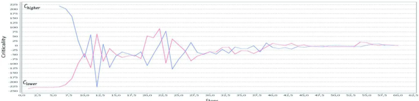
Firstly we propose to evaluate how the system behaves during the resolution process. Figure 3 shows the evolution of the criticalities of Chigher (green curve) and Clower (red
curve) during a simulation with 10 sensors. It illustrates the process of minimization of the criticalities by the cooperative behaviour of Weight agents. As the process goes along, new
Figure 3. Evolution of the criticality of Chigherand Clowerduring a run.
Constraint agents are added. Those agents might be more critical than the previous Constraint agents, explaining why at some points of the curves the criticalities increase. But when there is no change of the most critical Constraint agent, we observe a reduction of the criticalities and a convergence towards the value minimizing both criticalities. The more the problem becomes constrained, the more this value tends towards zero. This is visible at the end of the curves where both criticalities converge towards zero. This phenomenon is interesting as it allows to determine how the problem is constrained: the more criticalities of ChigherandClowertend
towards zero, the more constrained the problem is, and thus, the more precise the current weights should be.
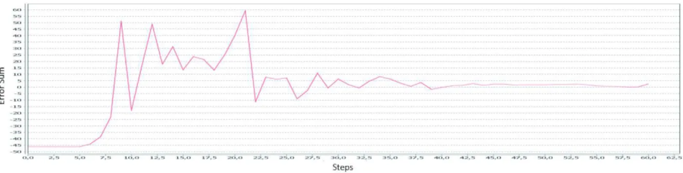
Figure 4 shows the difference in the computation of the degree of anomaly of the current situation P
n
ωt
n · ∆tn and
the degree of anomaly computed by the oracle P
n
ω∗ n · ∆tn.
The figure shows convergence towards zero, meaning that the MAS manages to estimate weights. By comparing this curve to the evolution of the criticalities ofChigher andClower, we
observe that the convergence towards zero of the criticalities ofChigherandClowercoincides with the convergence towards
zero of the difference of computation of the degree of anomaly of the current situation.
Algorithm 5 The meta-algorithm of one run of an experiment Require: The number of sensorsn, the bounds [ωmin, ωmax]
and[∆min, ∆max], the precision p to reach.
1: Initialize randomly the weightsω∗ of the oracle
2: Initialize the MAS and each of its weightsω at 1
3: nbStep ← 0 4: Computeprecision
5: whileprecision < p do
6: Send new disparity values to the MAS
7: Compute agents lifecycles
8: Receive decision from the MAS
9: Compute and send the oracle feedback
10: nbStep ← nbStep + 1 11: Computeprecision
12: end while
Then, we propose to evaluate MAS robustness to the pa-rameter sizen. For each sensor size value from 5 to 100 with a step of 5, we performed 100 different runs and computed the number of cycles to reach a minimum error of 3%. Figure 5 shows the results we obtained in the form of box plots showing the first quartileQ1, the median, and the third quartile Q3 for the 20 different parameter sizes. The figure shows a linear relation between the number of cycles required to reach the level of precision and the number of parametersn.
For each experiment, we also computed the number of Constraint agents that are actually selected as Chigher and
Clower and contribute to the solving process. Figure 6 shows
the results in the form of box plots. Once again, the number of actually used Constraint agents is linear with the number of parameters. Compared to the number of cycles required to reach the precision, the number of actually selected Con-straint agents is significantly lower. Indeed, not all ConCon-straint agents are required to solve the problem, only those which constrained the process. In this experiment, constraints are randomly created and there is no guarantee that new Con-straint agents are going to constrained the problem. Indeed, a newly created Constraint agent is not necessarily the most constrained agent, and thus may never be selected. But as the system evolves, it is not possible to make any assumption on the utility of a Constraint agent, as its constraint might not be respected anymore during the resolution process and thus become selected. The presence of those Constraint agents in the systems acts as a tool of anticipation, their activity ensures that the system will not be in a non cooperative state. Thus, the collective of Constraint agents acts as an heuristic guiding the system towards the solution. The main advantage of this approach is that this heuristic is dynamic and able to deal with the dynamic creation of Constraint agents.
V. CONCLUSION AND PERSPECTIVES
In this paper, we introduce a novel model for behavioural anomaly detection in the context of elderly people health-care. This model is based on the building of a Circadian Activity Rhythm on each sensor and its comparison with a nominal profile. Anomalies are detected through a linear regression. The adaptation of this model consists in finding the optimal weight parameters ω∗
Figure 4. Evolution of the difference of computation of the degree of anomaly of a situation Dtbetween the MAS and the oracle.
express the problem of adaptation as a problem of linear optimization using medical feedback to dynamically build a set of inequalities acting as constraints. The successive resolution of those inequalities acts as a heuristic guiding the system towards the optimal parameters. We propose an adaptive multi-agent model to dynamically resolve those inequalities.
The experiments performed on synthetic environments have shown both the capacity to achieve a certain level of precision in weight adjustment and that there exists a linear relation between the number of parameters and the number of cycles to find optimal parameters. However, while being promising, those experiments do not include noisy data or wrong feed-back, which might lead to the impossibility to find a solution that satisfies all the constraints. A real world experiment is ongoing, involving the monitoring of 20 patients at home over 3 months. Each home is equipped with a set of sensors enabling to monitor various aspects of the every day life of the elderly, such as the opening and closure of doors, presence sensors in each room and sensors to monitor water usage. The gathering of those data will allow the experimentation of the approach with real world anomalies, and will have to take into account this noise by giving the system the ability to release constraints. This real world experiment will also evaluate the acceptability of the solution for both patients and the medical staff.
ACKNOWLEDGEMENT
This work is part of the research project 3Pegase funded by the European Regional Development Fund and the French Occitanie Region. We would also like to thank our partners in this project: Telemedicine Technologies, Telegrafik, the Toulouse G´erontopˆole (Toulouse University Hospital), Orange and IMA Protect.
REFERENCES
[1] G. Virone, N. Noury, and J. Demongeot, “A system for automatic measurement of circadian activity deviations in telemedicine,” IEEE
Transactions on Biomedical Engineering, vol. 49, no. 12, pp. 1463– 1469, 2002.
[2] Y. Fouquet, C. Franco, J. Demongeot, C. Villemazet, and N. Vuillerme, “Telemonitoring of the elderly at home: Real-time pervasive follow-up of daily routine, automatic detection of outliers and drifts,” in Smart
Home Systems. InTech, 2010.
Figure 5. Box plot showing (x axis) the number of cycles to reach a minimum error of3% for (y axis) 20 different parameter sizes (from 5 to 100) with 100 runs for each n value.
Figure 6. Box plot showing (x axis) the number of actually used Constraint agents for (y axis) 20 different parameter sizes (from 5 to 100) with 100 runs for each n value.
[3] G. Virone, “Assessing everyday life behavioral rhythms for the older generation,” Pervasive and Mobile Computing, vol. 5, no. 5, pp. 606– 622, 2009.
[4] B. Kon, A. Lam, and J. Chan, “Evolution of smart homes for the elderly,” in Proceedings of the 26th International Conference on World Wide
Committee, 2017, pp. 1095–1101.
[5] H. Gokalp and M. Clarke, “Monitoring activities of daily living of the elderly and the potential for its use in telecare and telehealth: a review,”
Telemedicine and e-Health, vol. 19, no. 12, pp. 910–923, 2013. [6] P. Rashidi and A. Mihailidis, “A survey on ambient-assisted living tools
for older adults,” IEEE journal of biomedical and health informatics, vol. 17, no. 3, pp. 579–590, 2013.
[7] L. Nie, L. Zhang, Y. Yang, M. Wang, R. Hong, and T.-S. Chua, “Be-yond doctors: future health prediction from multimedia and multimodal observations,” in Proceedings of the 23rd ACM international conference
on Multimedia. ACM, 2015, pp. 591–600.
[8] M. L. Shahreza, D. Moazzami, B. Moshiri, and M. Delavar, “Anomaly detection using a self-organizing map and particle swarm optimization,”
Scientia Iranica, vol. 18, no. 6, pp. 1460–1468, 2011.
[9] H. Mshali, T. Lemlouma, and D. Magoni, “Adaptive monitoring system for e-health smart homes,” Pervasive and Mobile Computing, vol. 43, pp. 1–19, 2018.
[10] F. Bergenti and A. Poggi, “Multi-agent systems for e-health: Recent projects and initiatives,” in 10th Int. Workshop on Objects and Agents, 2009.
[11] V. Chan, P. Ray, and N. Parameswaran, “Mobile e-health monitoring: an agent-based approach,” IET communications, vol. 2, no. 2, pp. 223–230, 2008.
[12] G. B. Laleci, A. Dogac, M. Olduz, I. Tasyurt, M. Yuksel, and A. Okcan, “Saphire: a multi-agent system for remote healthcare monitoring through computerized clinical guidelines,” in Agent technology and e-health. Springer, 2007, pp. 25–44.
[13] D. Hern´andez, G. Villarrubia, A. L. Barriuso, ´A. Lozano, J. Revuelta, and J. F. De Paz, “Multi agent application for chronic patients: moni-toring and detection of remote anomalous situations,” in International
Conference on Practical Applications of Agents and Multi-Agent Sys-tems. Springer, 2016, pp. 27–36.
[14] V. Chandola, A. Banerjee, and V. Kumar, “Anomaly detection: A survey,”
ACM computing surveys (CSUR), vol. 41, no. 3, p. 15, 2009. [15] D. Capera, J.-P. Georg´e, M.-P. Gleizes, and P. Glize, “The amas theory
for complex problem solving based on self-organizing cooperative agents,” in Enabling Technologies: Infrastructure for Collaborative
Enterprises, 2003. WET ICE 2003. Proceedings. Twelfth IEEE Inter-national Workshops on. IEEE, 2003, pp. 383–388.
[16] N. Bonjean, W. Mefteh, M. P. Gleizes, C. Maurel, and F. Mi-geon, “Adelfe 2.0,” in Handbook on agent-oriented design processes. Springer, 2014, pp. 19–63.
[17] S. Lemouzy, V. Camps, and P. Glize, “Principles and properties of a mas learning algorithm: A comparison with standard learning algorithms applied to implicit feedback assessment,” in Proceedings of the 2011
IEEE/WIC/ACM International Conferences on Web Intelligence and Intelligent Agent Technology-Volume 02. IEEE Computer Society, 2011, pp. 228–235.