Modélisation et contrôle d'une main anthropomorphe actionnée par des tendons antagonistes

(1)

HAL Id: pastel-00957755

https://pastel.archives-ouvertes.fr/pastel-00957755

Submitted on 11 Mar 2014

HAL is a multi-disciplinary open access

archive for the deposit and dissemination of sci-entific research documents, whether they are pub-lished or not. The documents may come from teaching and research institutions in France or

L’archive ouverte pluridisciplinaire HAL, est destinée au dépôt et à la diffusion de documents scientifiques de niveau recherche, publiés ou non, émanant des établissements d’enseignement et de recherche français ou étrangers, des laboratoires

Modélisation et contrôle d’une main anthropomorphe

actionnée par des tendons antagonistes

Maxime Chalon

To cite this version:

Maxime Chalon. Modélisation et contrôle d’une main anthropomorphe actionnée par des tendons antagonistes. Autre. Ecole Nationale Supérieure des Mines de Paris, 2013. Français. �NNT : 2013ENMP0045�. �pastel-00957755�

(2)

T

H

È

S

E

INSTITUT DES SCIENCES ET TECHNOLOGIES

École doctorale nO_{432 :} Sciences des Métiers de l’Ingénieur

Doctorat ParisTech

T H È S E

pour obtenir le grade de docteur délivré par

l’École nationale supérieure des mines de Paris

Spécialité «Informatique temps-réel, robotique et automatique»

présentée et soutenue publiquement par

Maxime CHALON

le 2 octobre 2013

Modélisation et contrôle d’une main anthropomorphe actionnée

par des tendons antagonistes

∼ ∼ ∼

Modeling and control of an antagonistically actuated tendon

driven anthropomorphic hand

Directeur de thèse : Brigitte d’ANDREA-NOVEL

Jury

Maxime GAUTIER,Professeur, Faculté des Sciences et Techniques, Université de Nantes Rapporteur

Claudio MELCHIORRI,Professeur, Faculty of Engineering, University of Bologna Rapporteur

Brigitte d’ANDREA-NOVEL,Professeur, MINES ParisTech Examinateur

Markus GREBENSTEIN,Dr. Institute of Robotics and Mechatronics, DLR Examinateur

Christian OTT,Dr.-Ing. Institute of Robotics and Mechatronics, DLR Examinateur

Véronique PERDEREAU,Professeur, Université Pierre et Marie Curie Examinateur

MINES ParisTech Centre de robotique (CAOR)

(3)

(4)

Acknowledgment

To give acknowledgment to all the persons that supported this work is with-out a doubt a challenge on its own. I decided to list the people that helped under all forms, without specific order or importance. If you are missing, please be sure that it was not intentional. Thanks to: Brigitte d’Andreas-Novel for being my professor during this work. Jens Reinecke for the un-believable number of hours spent in experimenting together. Werner Friedl for building all the test setups and designing the forearm. Alex Dietrich for correcting so well all the little details and for the discussion on the possible control methods. Thanks to Thomas Wimbock with whom I started at DLR and that supported me for my first papers. Markus Grebenstein for creating this fantastic system. Alin Albu-Schaeffer for giving me the chance of work-ing in DLR and more generally to all the colleagues I have been discusswork-ing with.

(5)

(6)

5.3 Ring and fifth fingers . . . 84 5.3.1 Kinematic model . . . 84 5.3.2 Dynamic model . . . 84 5.3.3 Tendon coupling . . . 85 5.4 Thumb . . . 85 5.4.1 Kinematic model . . . 86 5.4.2 Dynamics model . . . 86 5.4.3 Tendon coupling . . . 87 5.5 Hematometacarpal joint . . . 91 5.6 Conclusion . . . 92 6 Wrist Model 95 6.1 Kinematic model . . . 95 6.1.1 Calculation of angle tC . . . 97 6.1.2 Calculation of angle tA. . . 100 6.2 Kinematic verification . . . 101 6.3 Conclusion . . . 104 II Control 107 7 Tendon force distribution 113 7.1 Problem formulation . . . 113 7.2 Solutions . . . 114 7.3 Discussion . . . 116 8 Stiffness correction 119 8.1 Problem formulation . . . 119 8.2 Adaptive Controller . . . 119 8.3 Challenges . . . 120

8.4 Simulation and experiments . . . 121

8.5 Discussion . . . 122

9 Joint torque observer 125 9.1 Structure . . . 125

9.2 Experimental setup . . . 126

10 Tendon control 129 10.1 Control model . . . 129

10.2 Controller design . . . 129

10.3 Gains scheduling design . . . 132

10.3.1 Linearized form . . . 132

(8)

10.3.3 Gain scheduled controller . . . 134

10.4 Experimental and simulation results . . . 134

11 Two time scale approach 137 11.1 Model . . . 137

11.2 Tendon Controller Design . . . 138

11.3 Link Controller Design . . . 138

11.4 Stability Conditions: The singular perturbation case . . . 139

11.5 Stability Conditions : The cascaded case . . . 141

11.6 Experimental Results . . . 142

12 Direct pole placement 147 12.1 Introductory example . . . 148

12.2 Fourth order model . . . 149

12.3 Robustness analysis . . . 151

13 Optimal control 155 13.1 Introduction example . . . 155

13.2 Fourth order system . . . 156

13.3 Simulation . . . 157

14 State-Dependent Riccati Equation 161 14.1 State Dependant Riccati Equations . . . 162

14.2 Applications . . . 162

14.2.1 Tendon force controller . . . 163

14.2.2 Flexible joint model . . . 164

14.3.1 Application to a tendon force controller . . . 165

14.3.2 Application to a joint controller . . . 165

14.4 Discussion . . . 166 15 Backstepping 169 15.1 Concept . . . 170 15.1.1 Controller design . . . 170 15.1.2 Simulations . . . 171 15.1.3 Conclusion . . . 172

15.2 Single ﬂexible joint: position controller . . . 172

15.2.1 Model . . . 172

15.2.2 Strict Feedback Form . . . 175

(9)

15.2.4 Simulations . . . 180

15.2.5 Experiments . . . 186

15.2.6 Conclusion . . . 188

15.3 Single ﬂexible joint: impedance . . . 188

15.3.1 Model . . . 189

15.3.2 Controller . . . 189

15.3.3 Simulations . . . 192

15.3.4 Experiments . . . 193

15.3.5 Conclusion . . . 193

15.4 Single ﬂexible joint: impedance non linear stiﬀness . . . 194

15.4.1 Model . . . 195 15.4.2 Controller . . . 196 15.4.3 Simulations . . . 197 15.4.4 Experiments . . . 198 15.4.5 Conclusion . . . 198 15.5 Antagonistic joint . . . 199 15.5.1 Model . . . 201 15.5.2 Simulations . . . 204 15.5.3 Experiments . . . 204 15.5.4 Conclusion . . . 207 15.6 Conclusion . . . 207 16 Optimal backstepping 209 16.1 State-feedback transformation . . . 210

16.2 Optimal problem formulation . . . 210

16.3 Solution . . . 210

16.4 Simulation . . . 211

16.5 Experiments . . . 213

(10)

List of Figures

1.1 Aerial View of the DLR site in Oberpfaﬀenhofen (courtesy of

DLR) . . . 25

1.2 General View of the System . . . 26

1.3 Left: Humanoid Asimo from Honda. Right: Second version of the HRP humanoid from Kawada Industries . . . 28

1.4 Two humanoid robots . . . 29

1.5 Ri Man, a health care robot designed by Riken in Japon . . . 30

1.6 Two upper humanoids . . . 30

1.7 Wendy and TwendyOne . . . 31

1.8 Two early tendon driven hands . . . 32

1.9 UB3 . . . 32

1.10 Dexhand a space qualiﬁable hand from DLR . . . 33

1.11 Kojiro . . . 34

1.12 Workspace analysis for the thumb of the hand of the Hand Arm System . . . 35

1.13 Simulation tool for grasp evaluation: GraspIt! . . . 36

1.14 Datasheet from the VIACTOR project . . . 37

1.15 VSA-HD. . . 38

1.16 Overview of the structure of the thesis . . . 41

1.17 Overview of the structure of the modeling part . . . 47

2.1 Isolated link i . . . 51

3.1 Rendered motor module and real motor module . . . 55

3.2 Motor model . . . 56

3.3 Experiment and results for the motor friction estimation . . . 59

3.4 Experiment: commanded torque for constant velocity motions 60 3.5 Experiment: commanded torque for a constant velocity mo-tion (time and frequency domains) . . . 61

3.6 Experiment: resulting controller torque command in time and frequency domains after compensation . . . 61

4.1 Antagonistic arrangement of the tendons allowing to move the joint and adjust its stiﬀness . . . 64

4.2 Antagonistic driving principle . . . 64

4.3 Durability test of diﬀerent tendon material depending on the pulley radius . . . 65

4.4 Splicing technique used to terminate the tendons . . . 65

4.5 Original concept: tangent α mechanism . . . . 66

4.6 Geometry of the tendon force sensor: the stiﬀness is increas-ing from left to right . . . 66

(11)

4.7 Model based mechanism characteristics . . . 67

4.8 Tendon force/stiﬀness calibration . . . 68

4.9 Experiment for guiding friction estimation . . . 69

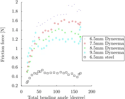
4.10 Friction force depending on the total bending angle . . . 70

4.11 Friction coeﬃcient in a sliding experiment . . . 70

5.1 Joint names . . . 74

5.2 Hyperboloid joint of the ﬁnger base . . . 74

5.3 Dislocatable hinge joint for the PIP and DIP joints . . . 75

5.4 Tendon routing of the index ﬁnger through the complete forearm 75 5.5 Index ﬁnger of the Hand Arm System . . . 77

5.6 Frame deﬁnition of the index ﬁnger of the Hand Arm System (side view) . . . 77

5.7 Simulation: inﬂuence of the Coriolis and centrifugal terms on the link trajectory . . . 80

5.8 Names of the tendons and radii of the pullies of the index ﬁnger used to establish eq. (5.22). . . 81

5.9 Antagonistic model of a joint. Two motors are pulling two tendons guided through the stiﬀness elements and drive the joint (courtesy of Jens Reinecke). . . 82

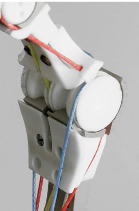
5.10 Example of the tendon guiding in the PIP and DIP . . . 82

5.11 Mechanical realization of the PIP/DIP coupling of the ring and fifth fingers (case of the ring finger) . . . 85

5.12 Thumb of the Hand Arm System . . . 86

5.13 Joint axis and tendon names of the thumb of the Hand Arm System . . . 87

5.14 Thumb of the Hand arm system . . . 88

5.15 Structure of the coupling matrix . . . 90

5.16 Link position estimation : gradient search . . . 92

5.17 Results of the link position estimation with diﬀerent step sizes and step counts . . . 93

6.1 Wrist of the hand arm system. The two groups of 19 tendons are going through the wrist . . . 96

6.2 Side view of the wrist (CAD) . . . 96

6.3 Top view of the wrist (CAD) . . . 97

6.4 BC plane transformation (CAD) . . . 97

6.5 Distance constraints between B and C in the plane . . . . . 98

6.6 BC plane transformation . . . 99

6.7 BC plane transformation with α = 30 deg (CAD) . . . . 99

6.8 Palm frame ABC . . . 101

6.9 Simulation: maximum error on the distance constraints . . . 103

6.10 Simulation: calculated tendon displacement resulting from a wrist motion . . . 104

(12)

6.11 Experiment: measured tendon displacement resulting from the recorded wrist motion . . . 105 6.12 Experiment: simulated tendon displacement resulting from

the recorded wrist ﬂexion/extension motion . . . 105 6.13 Experiment: measured tendon displacement resulting from

the recorded wrist abduction/adduction . . . 106 6.14 Overview of the structure of the control part . . . 110 8.1 Serial interconnexion of the controller stiﬀness and the

me-chanical stiﬀness . . . 120 8.2 Control structure used for adjusting online the impedance

gain to obtain the desired effective impedance. . . 121 8.3 Effective stiffness using the active correction. The red/solid

curve depicts the impedance controller stiffness. The blue/dotted curve represents the mechanical stiffness. The green/dashed dotted curve depicts the resulting, nearly constant, stiffness. . 122 9.1 Structure of the link side friction observer . . . 126 9.2 Placement of the stain gauges in the index finger . . . 126 9.3 Joint tracking performance in simulation (top) and in

experi-ments (bottom). A sinusoidal trajectory, represented in light blue/dotted is used as reference joint trajectory. The eﬀective joint motion is represented in red/solid. The estimated joint friction torque is depicted by the green/dashed-dotted curve. 128 10.1 Simulation: force step response of the plant with and

with-out feedforward terms. The dotted/green curve denotes the desired force. The blue/dashed curve represents the force without feedforward term. The solid/red curve represents the force with feedforward term. . . 130 10.2 Force step response of the controller whose gains are tuned for

30 N. The gains are tuned to obtain the fastest settling time without overshoot. In each experiment, only the initial ten-don force and the target tenten-don force are modiﬁed. It can be observed that the response is ideal for 30 N but underdamped for 10 N and 20 N. . . 131 10.3 Simulations: Tendon force control with/without adaptive gains.

In both figures, the measured and desired tendon force is de-picted. A step of 5N is commanded from different initial states. The adaptive controller is superior to the fixed gain controller except for the lowest force which is due to the satu-ration of the control input. The fixed gain controller is tuned for 30N. . . 135

(13)

10.4 Experiments: Tendon force control with/without adaptive gains. In both figures, the measured and desired tendon force is depicted. A step of 5N is commanded from different initial states. The adaptive controller is superior to the fixed gain controller for all the cases. The fixed gain controller is tuned

for 30N. . . 135

11.1 Tendon force controller experiments . . . 139

11.2 Experiment: step response for two impedance controller stiﬀ-ness . . . 143

11.3 Experiment: step response for two different mechanical stiffness144 11.4 Experiments: shift of the resonance according to the stiffness of the link . . . 144

12.1 Simple mass spring damper system . . . 148

12.2 Double spring mass damper system in the case of a ﬂexible joint model . . . 149

12.3 Root locus of the open loop plant . . . 153

12.4 Root locus of the closes-loop plant . . . 153

13.1 Single mass-spring-damper. . . 155

13.2 Simulation: link and motor trajectories of the plant under an optimal state feedback controller. The simulations per-formed with R = 0.0001 (resp. 0.01 and 1 are denoted by A/red (resp. B/light blue, C/green). The solid line represents the motor position whereas the dotted line represents the link position. . . 158

13.3 Simulation: input command of the plant under an optimal state feedback controller. The curves A/red (resp. B/light blue, C/green) are corresponding to the simulations of Figure 13.2. . . 159

14.1 Model for the tendon force controller. The link is assumed to be ﬁxed, thus the tendon force only depends on the motor position. . . 163

14.2 Flexible joint model . . . 164

14.3 Simulation: Comparison SDRE and ﬁxed gains, tendon force 167 14.4 Simulation: Comparison SDRE and ﬁxed gains, link . . . 167

14.5 Simulation: Comparison SDRE and ﬁxed gains, gains . . . . 168

15.1 Simulation results: x1 trajectories obtained for diﬀerent val-ues of k1 and k2. Slice are for k1 ∈ [0.01, 2.0, 5.0, 7.5, 10.0]. Colors are for k2 ∈ [0.5, 1.55, 2.61, 3.67, 4.72, 5.78, 6.83, 7.89, 8.94, 10.0]. Initial conditions are x1 = 1, x2 = 1. . . 172

(14)

15.2 Simulation results: solution trajectories for diﬀerent initial conditions represented in a phase diagram of ˙x1(x1).

Feed-back gains are k1 = 0.1, k2 = 5. Initial conditions are marked

by a cross symbol. . . 173 15.3 Simulation results: solution trajectories for diﬀerent initial

conditions represented in a phase diagram of ˙x1(x1).

Feed-back gains are k1 = 1, k2 = 1. Initial conditions are marked

by a cross symbol. . . 173 15.4 Simulation results: solution trajectories for diﬀerent initial

conditions represented in a phase diagram of ˙x1(x1).

Feed-back gains are k1 = 5, k2 = 0.1. Initial conditions are marked

by a cross symbol. . . 174 15.5 Double spring mass damper system in the case of a ﬂexible

joint model. . . 174 15.6 Graphical representation of the state transition matrix of a

system in strict feedback form. . . 175 15.7 Simulations, inﬂuence of K1: link position after a commanded

step of 0.8 rad. The red/solid, light blue/dashed, blue/dot dashed and orange/dotted lines depict the responses obtained for a gain K1 of 0.2, 1, 5 and 50 (the K2 coeﬃcient being set

to K2 = 1). The coeﬃcient K1 has a strong inﬂuence on the

stiﬀness of the link. . . 182 15.8 Simulations, inﬂuence of K2: link position after a commanded

step of 0.8 rad. The red/solid, light blue/dashed, blue/dot dashed and orange/dotted lines are representing the link po-sition obtained for a K2 coeﬃcient of 0.2, 1, 5 and 50 (the

K1 coeﬃcient being set to K1= 5). The coeﬃcient K2 has a

strong inﬂuence on the damping of the link. . . 183 15.9 Diagram of the simulation used for the evaluation of the

inﬂu-ence of input saturation. A saturation block is placed between the controller output and the plant. . . 183 15.10Simulations, inﬂuence of a saturation of the control input u:

link position after a commanded step of 0.8 rad. The red/solid and light blue/dashed curves are the responses obtained with-out and with a saturation of|u| < 0.0005 (the coeﬃcients are set to K1= 1, K2 = 1, K3 = 100 and K4 = 100). . . 184

15.11Simulations, inﬂuence of a saturation of the control input u: input command after a commanded step of 0.8 rad. The light blue(solid) and blue (dashed) lines are the responses obtained without and with a saturation of_{|u| < 0.0005 (the coeﬃcients} are set to K1= 1, K2= 1, K3= 100 and K4 = 100). . . 185

(15)

15.12Diagram of the simulation used for the evaluation of the in-fluence of time delays. A fixed delay is placed between the command and the actuator as well as between the measure-ments and the controller. . . 185 15.13Simulations, influence of a delay in the control input u: link

position after a commanded step of 0.8 rad. The red/solid (resp. light blue/dashed, blue/dotted, orange/dot dashed) line is the response obtained with a 0ms delay (resp. 0.1, 0.2, 0.5 and 1ms) (the coeﬃcients are set to K1 = 5, K2 = 1,

K3= 100 and K4 = 100). . . 186

15.14Experimental setup used for the veriﬁcation of the backstep-ping controller . . . 187 15.15Experiment: measured motor position red/solid and link

po-sition light blue/dotted after a commanded popo-sition step. The pulley ratio between the motor and the link is about 3. Left: a PD controller on the motor position is used. Right: the backstepping controller is used. . . 187 15.16Simulation: influence of the stiffness coefficient . . . 192 15.17Simulation: influence of the damping coefficient . . . 193 15.18Experiment: measured and expected joint torque w. r. t. an

increasing joint position error from 0 to 0.5 rad. . . 194 15.19Simulation: comparison between the linear backstepping

con-troller and the nonlinear backstepping concon-troller on a nonlin-ear plant. The solid/red curve depicts the link position under the nonlinear controller. The dashed/green curve depicts the link position under the linear controller. . . 197 15.20Simulation: change of the joint stiﬀness during the

experi-ment depicted in Fig. 15.19. The solid/red curve depicts the link position under the nonlinear controller. The dashed/green curve depicts the link position under the linear controller. The stiffness change when accelerating the link (cf. point A, at t = 0.5s) is negligible w. r. t. the change of stiffness imposed by the external load (at time t = 1.5s). . . 198 15.21Simulation: effect of a motor torque saturation on the

con-trollers. The solid/red curve depicts the link position under the nonlinear controller. The dashed/green curve depicts the link position under the linear controller. In both cases, a saturation is applied on the motor torque. The diﬀerence be-tween the two controller is reduced. Nonetheless, the settling time of the nonlinear controller remains shorter. . . 199

(16)

15.22Experiment: measured link side position and joint torque af-ter a desired position step of 1.3 rad and exaf-ternal obstacle placed at 0.8 rad. Between 0s and 2s the impedance gain is 0.5Nm/rad (in red). The impedance gain is 5Nm/rad between

2s and 4s (in blue). . . 200

15.23Antagonistic backsteppping controller behavior . . . 204

15.24Step response backstepping controller PIP joint . . . 205

15.25Sinus tracking backstepping controller PIP joint . . . 205

15.26Gain diagram backstepping and singular perturbation controller206 15.27Veriﬁcation of the impedance behavior . . . 207

16.1 Simulation model for a ﬂexible joint with linear springs . . . 211

16.2 Simulations: joint behavior for diﬀerent samples of gains. The desired link position is depicted in red/solid and the measured joint position in light blue/dashed. The external joint torque is traced in green/dotted and the joint torque is represented in black/dashed-dotted. . . 212

16.3 Experiments: joint behavior for diﬀerent samples of gains. The measured joint position are reported. . . 214

(17)

(18)

List of Tables

2.1 Symbols and units . . . 50

3.1 Diﬀerent contributions to the total motor friction . . . 56

3.2 Parameters to be identiﬁed . . . 57

3.3 Parameters of the friction model . . . 58

4.1 Parametrization of the spring mechanism . . . 67

5.1 Transformations from index base to index ﬁngertip . . . 78

5.2 Coordinates of the bone insertion points for the tendons . . . 88

6.1 Wrist symbol deﬁnitions, units and values . . . 96

6.2 Tendon oﬀset in the forearm frame and in the palm frame . . 102

12.1 Numerical values used to evaluate the poles . . . 152

13.1 Parameters used for the simulation of the optimal state feedback157 14.1 Simulation parameters for the tendon controller . . . 165

14.2 Simulation parameters for the joint controller . . . 165

15.1 Simulation parameters for a single joint and single motor with linear stiﬀness . . . 181

15.2 Experimental parameters and controller parameters for a sin-gle joint and sinsin-gle motor with linear stiﬀness . . . 187

16.1 Numerical values for the simulations . . . 212

(19)

(20)

Résumé

Ce chapitre résume les points importants de chaque chapitre de ce manuscrit.

Introduction

Pour commencer, une courte présentation de DLR ainsi que du récent sys-tème bras-main (appelé Hand Arm System) est donnée.

Ce nouveau système a la particularité d’être mécaniquement flexible. Cette flexibilité intrinsèque offre la possibilité de stocker de l’énergie à court terme et remplit ainsi deux fonctions essentielles pour un robot humanoïde: les impacts sont filtrés et les performances dynamiques sont augmentées. Dans cette thèse, on se concentre plus particulièrement sur la main. Chacun des 19 degrés de liberté est actionné par deux tendons flexibles antagonistes. La rigidité des tendons étant non linéaire il est possible, tout comme peut le faire l’être humain, de co-contracter les " muscles " et ainsi de modifier la rigidité mécanique. Il est donc possible d’ajuster la rigidité des doigts afin de s’adapter au mieux aux tâches à effectuer. Cependant, cette flexibilité entraine de nouveau défis de modélisation et de contrôle.

De nombreuses mains robotiques ont été développées au centre de robo-tique de DLR et dans d’autres laboratoires à l’international. Le système est unique à la fois par sa complexité, utilisant 42 moteurs et plus de 200 capteurs, et par sa construction mécanique unique. Les travaux publiés se concentrent majoritairement sur le problème de la répartition des forces internes ou alors du contrôle d’articulation flexible mais peu de travaux con-sidèrent les deux problèmes simultanément. Les travaux sont présentés en deux parties. La première se concentre sur la modélisation tandis que la seconde concerne le contrôle. Autant que possible, des simulations et des mesures sont réalisées afin de vérifier la validité des hypothèses.

Modeling and identification

Cette première partie vise à établir des modèles mécaniques pour l’ensemble des sous-systèmes. Puisque le système comporte plus de 50 moteurs et 200 capteurs, une démarche bottom-up est utilisée.

Modeling approach

Les méthodes utilisées pour la modélisation sont présentées. La cinéma-tique est construite grâce à des transformations homogènes. Pour le modèle dynamique deux approches principales sont présentées. Les avantages et désavantages de plusieurs méthodes sont discutés. Finalement, il est vériﬁé

(21)

que les termes représentant les forces de Coriolis et centrifuge peuvent être négligés.

Motor model

Le système utilise un total de 38 moteurs pour tirer et relâcher les tendons. Il est important de disposer d’un modèle précis du comportement des moteurs aﬁn de pouvoir contrôler les forces ou les positions des tendons. Un modèle des frottements périodiques générés par l’engrenage harmonique est établi et il est montré qu’un compensateur permet de réduire sensiblement les vibrations.

Tendon model

Les articulations sont actionnées par des tendons ﬂexibles. Le déplacement et la force d’un tendon sont mesurés par un capteur magnétique placé sur le ressort. Le ressort est linéaire mais est placé dans un mécanisme générant une relation non linéaire. Le mécanisme est modélisé et des mesures sont eﬀectuées pour sélectionner les paramètres du modèle.

Finger model

La structure mécanique des doigts est similaire à l’exception du pouce et de l’articulation distale de l’annulaire. Le chapitre propose un modèle cinéma-tique pour chacun des doigts. Les équations qui permettent de transformer les forces et les positions des tendons pour obtenir le couple et la rigidité de l’articulation sont établies. Les articulations des doigts ne disposent pas de capteur, cependant puisque huit tendons sont utilisés pour actionner quatre articulations, un algorithme est nécessaire pour évaluer la position des doigts à partir du déplacement des tendons. Le cas spécial du pouce est présenté car l’insertion des tendons est différente afin de produire une force suffisante pour s’opposer aux autres doigts. La relation géométrique non linéaire entre le déplacement des tendons et le déplacement des articulations requière un algorithme particulier. L’algorithme est présenté accompagné de simulations visant à estimer sa vitesse de convergence.

Wrist model

L’ensemble des tendons est guidée au travers du poignet. Cependant, puisqu’il est mécaniquement impossible de faire passer tous les tendons par un unique centre de rotation, un déplacement du poignet implique un déplacement des tendons. Si le déplacement n’est pas compensé, un mouvement des doigts est perceptible. La modélisation de la cinématique du poignet est présentée étape par étape. Finalement, des mesures sont eﬀectuées et comparées aux simulations.

(22)

Control

La seconde partie utilise les modèles pour établir les lois de contrôle. Les premiers chapitres présentent deux problèmes spécifiques aux systèmes ac-tionnés par tendons. Ensuite, un régulateur pour la force des tendons est développé et expérimenté. Dans un premier temps, un contrôleur pour la force des tendons est construit. Ensuite, similaire aux approches proposées dans la littérature, un contrôleur en cascade, basé sur le régulateur de force des tendons, est présenté et analysé. Afin de s’affranchir de l’hypothèse de cascade, une approche classique de placement de pôles est envisagée. Le choix des gains étant une étape critique pour un système avec 38 moteurs, une méthode de contrôle optimal basé sur les équations de Riccati est pro-posée. Puisque que le système est non linéaire, la méthode SDRE (State Dependant Riccati Equation) est utilisée. Les méthodes proposées jusqu’à ce point sont linéaires ou du moins, motivées par une approche linéaire. Afin d’explorer de nouvelles possibilités, une approche strictement non linéaire est exposée. La méthode porte le nom de backstepping. Finalement, la ques-tion du choix des gains pour le backstepping est détaillée et une méthode est proposée pour automatiser ce choix.

Tendon force distribution

Comme pour la majorité des systèmes actionnés par tendons, il est primor-dial de s’assurer que les forces des tendons restent bornées. Dépasser la force maximale admissible augmente le risque de rupture. Inversement, une force trop faible augmente le risque qu’un tendon quitte ses guides. Dans un système actionné par des tendons antagonistes flexibles, il existe une infinité de combinaison de forces qui produisent les mêmes couples. Il est possible d’ajuster la rigidité mécanique du système en modifiant les forces internes. Le chapitre présente plusieurs formulations du problème et discute plusieurs méthodes permettant de distribuer les forces.

Stiffness correction

Les tendons étant flexibles, ils apportent une flexibilité mécanique aux doigts. De plus, en pratique, un contrôleur d’impédance est utilisé pour augmenter les possibilités d’ajustement. Cependant, puisque la flexibilité mécanique et la flexibilité apportée par le contrôleur sont connectées en série, l’utilisateur perçoit une combinaison des deux. Le chapitre modélise cette connexion et propose un contrôleur adaptatif afin de produire la flexibilité désirée par l’utilisateur.

(23)

Joint torque observer

Aucun capteur n’est placé en dehors de l’avant bras ce qui confère aux doigts une excellente robustesse. Ils sont à la fois résistants aux impacts et insensi-bles à la poussière et à l’humidité. En contre partie, les frottements induits par les articulations et qui ne sont pas mesurés, réduisent la sensibilité des doigts. Il est possible d’estimer les frottements des articulations en ajoutant des capteurs de contrainte sur la structure des doigts. Il est ainsi possible d’analyser la contribution des frottements des articulations et d’estimer les gains possibles par une amélioration des articulations.

Tendon control

Bien que de nombreuses approches soient disponibles, la plupart des con-trôleurs sont basés sur un contrôle de la force des tendons. Ce chapitre établi plusieurs lois de contrôle pour la régulation de la force des tendons. Puisque la rigidité des tendons est non linéaire, la réponse d’un contrôleur linéaire dépend du point de fonctionnement. Une modification du contrôleur, in-spirée par la méthode de " Gain Scheduling " est proposée et les expériences confirment que la méthode est effective.

Two time scale approach

La méthode la plus directe pour créer un contrôleur d’impédance pour les articulations consiste à considérer deux problèmes indépendants. Le premier consiste à calculer un couple de référence pour les articulations, tandis que le second consiste à générer les forces correspondantes pour les tendons. La stabilité du système est simple à prouver s’il est admis que les échelles de temps sont suffisamment différentes. Les échelles de temps dépendent de la rigidité mécanique du système et donc la validité de l’approche dépend des contraintes internes. Une analyse plus complexe grâce à la théorie des systèmes en cascade permet de garantir la stabilité en contrepartie d’un choix plus difficile des matrices de gains.

Pole placement

Pour des systèmes d’ordre élevé, il est difficile de choisir les gains de re-tour d’état. Dans le cas d’une approche linéaire il est possible de placer les pôles du système afin de garantir sa stabilité. Il suffit pour cela de choisir les gains pour obtenir des parties réelles négatives pour les pôles. Bien que théoriquement correct, la méthode ne prend pas en compte les limites réelles du système tel que les délais de calculs, le bruit de mesure ou encore la sat-uration des actionneurs. En conséquence, la méthode est délicate à utiliser car des pôles peu réalistes nécessitent une action de contrôle impossible à réaliser.

(24)

Optimal control

Le chapitre étudie la question du choix des gains en utilisant des résultats de contrôle optimal. Grâce aux équations de Riccati il est possible d’obtenir les gains optimaux pour le contrôle du système linéaire.

State-Dependent Riccati Equation

Les équations de Riccatti ne s’appliquent qu’à des systèmes linéaires. Néan-moins, une extension aux systèmes non linéaire a été proposé sous le nom de State-Dependent Riccati Equation. Elle consiste à linéariser le système en tout point et à appliquer la méthode de Riccati. Des simulations sont présentées pour évaluer le gain de performance par rapport à la méthode de Riccati utilisée pour le système nominal.

Backstepping

Le backstepping est une méthode de contrôle non linéaire pouvant s’appliquer à une large gamme de systèmes. Elle présente l’avantage de ne pas nécessiter de linéarisation et permet d’établir la stabilité du système en boucle fermée. Un contrôleur d’impédance est souhaité pour les articulations et donc le backstepping est modiﬁé pour produire le comportement attendu. La méth-ode est appliquée pas à pas à des systèmes de plus en plus complexes. La stabilité est établie par construction au travers d’une fonction de Lyapunov. Des expériences et les simulations correspondantes sont présentées et attes-tent de l’applicabilité de la méthode. Finalement, la méthode est appliquée à une articulation antagoniste et des mesures conﬁrment qu’un contrôleur d’impédance est obtenu et a une performance supérieure aux contrôleurs précédant.

Optimal Backstepping

Le contrôleur de backstepping a une très bonne performance mais, tout comme le placement de pôle, est diﬃcile à paramétrer. Le chapitre propose d’identiﬁer les gains du contrôleur à ceux d’un contrôleur d’état optimal. Le résultat est une méthode permettant de sélectionner automatiquement les gains en fonction de matrices de coût.

Conclusion

Le Hand Arm System est un nouveau système qui permet d’explorer de nou-velles méthodes de manipulation de par sa robustesse et son dynamisme. Le travail présenté dans ce manuscrit s’est concentré sur la main et le poignet.

(25)

Il couvre la modélisation et le contrôle. De nombreuses expériences et sim-ulations sont présentées et il est montré que des méthodes non linéaires peuvent être appliquées aﬁn de maximiser les performances.

(26)

1 Introduction

1.1 DLR

The work presented in this thesis is realized at the Institute of Robotics and Mechatronics of the German Aerospace Center (Deutsche Luft and Raum-fahrt DLR). The institute focuses on research in the ﬁeld of robotics, ranging from industrial robot control to innovative biped platform and targets ser-vice robotic applications as well as space robotics. About 300 reseachers and students are working on mechanical design, electronics, control, perception, and planning. The institute is located near Munich (Oberpfaﬀenhofen) in Germany (cf. Fig. 1.1).

Figure 1.1: Aerial View of the DLR site in Oberpfaﬀenhofen (courtesy of DLR)

1.2 The Hand Arm System

The Hand Arm System (cf. Fig. 1.2) is composed of an arm, a wrist and a hand [1]. The arm has five degrees of freedom1 (DoFs) for the arm motion and five DoFs for the adjustement of the stiffness, thus actuated by a total of 10 motors. The wrist is actuated by four motors, in a helping antagonism configuration [2], and provides 2 DoFs of motion and 2 DoFs of stiffness. Finally, the hand is composed of 5 fingers and 19 joints, with 4-4-4-3-4 DoFs of motion (and 4-4-4-3-4 DoFs for adjusting the stiffness), actuated by 38 motors located in the forearm. The motor motion is transferred to the finger joints by tendons. A tendon is routed through a pulley/spring mechanism that provides a mean to adjust the joint stiffness by changing the tendon pretension [3]. Similarily, all joints of the arm are equiped with nonlinear spring mechanism, thus are able to modify the arm mechanical 1_{In robotics, the number of degree freedom is the mininal number of parameters needed}

(27)

stiﬀness. The system is the basis for a new generation of humanoid robots.

Figure 1.2: General View of the System

Not only it is looking human in size and shape, but it can also compete with the human in terms of force, accuracy and speed. The design and the realization of a system of such a complexity was only possible because of the very high integration of all components and a tight collaboration between the team members. From the concepts to the ﬁnal system, the entire robot has been design and manufactured in DLR, ensuring the quality and the ﬁt of all components.

1.3 Motivation

1.3.1 Robustness

It seems that several major challenges in robotics such as grasping, manipu-lation and mobility are still not tackled because the robustness of robots is often too limited. Considering the fact that the failure rate increases with the robot complexity, the number of parts and the diminution of part size, it is not surprising that hands are often in need for maintenance, severely restricting the operational time and the associated progress. One of the major targets of the development of the Hand Arm System is to develop a humanoid robotic system that is able to operate in a partially unknown environment, which poses strong demands on the robustness of the design. Hard collisions with other objects are unavoidable and the successful oper-ation of such a system is strongly related to the ability to withstand those collisions, and impacts, without severe damage or functional impairments.

Generally, the system complexity of robotic systems has been drastically increasing, simultaneously rising the risk of system failure. A single

(28)

colli-sion during operation may lead to a significant maintenance time and the associated costs. Therefore, application developers have to be conservative when testing new methods and strategies. This slows down progress and hardly gives a chance to develop radically different control/motion plan-ning strategies. In robotic hands, the impact tolerance plays an even more dominant role than in robot arms since during grasp acquisition or tactile exploration, the fingers are strongly exposed and a fragile hardware simply prohibits many strategies.

The elasticity in the fingers increases the robustness. An experiment showing how the fingers resisted to the impact of a hammer hit has been realized. In a similar fashion, the arm has been hit by a baseball bat and the joints accelerations were recorded. The measurements demonstrated that, without the mechanical compliance, the system could not continue operating (the impact exceeds the gear box peak load capability). Those experiments have a good media impact, moreover, they demonstrate that the fragility of non-industrial robots can be greatly improved without significant increase in weight, size or cost (often at the expense of control complexity). Several videos demonstrating the robustness of the system have been released on public media platforms such as YouTube (e. g. YouTube: Robot Arm Using a Hammer).

1.3.2 Dynamics

Interesting to notice, is the fact that the dynamic capabilities of current state-of-the-art robots are not comparable to human capabilities in terms of speed at the same inertial properties [4]. Particularly in cyclic tasks (e. g. running) or highly dynamic tasks (throwing, kicking), the energy the actu-ators can provide during peak loads without getting too bulky and heavy is not sufficient. In contrast to the classical stiff robots, elastic actuation can generate more output power, for a short time, than the maximum motor power. It enables to consider an entirely new set of mechanical designs, motion control schemes, and control strategies. For example, by explicitly controlling the potential energy that can be stored in the joint and trans-forming it to kinetic energy, i. e. link speed. This explicit use of the elasticity for highly dynamic motions constitutes a major step for equipping service robots with human like motion capabilities. Some initial work done in [5–7], identified this property and used it on a rather conceptual level. More re-cently, several control schemes were proposed to explicitly maximize the dynamic range of variable stiffness robots [5, 8–10].

These recent works show very promising results that pose several new re-search questions; How to optimize the control to maximize the power output during explosive motions (e. g. throwing a ball), how to damp the oscillations resulting from the low mechanical stiffness, and how to set the stiffness in order to achieve energy efficient motions. The, short term, energy storage

(29)

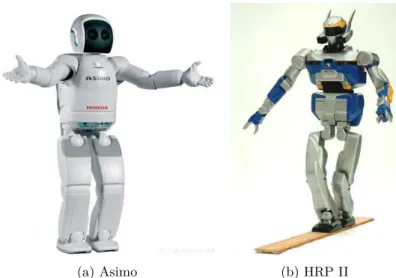
(a) Asimo (b) HRP II

Figure 1.3: Left: Humanoid Asimo from Honda. Right: Second version of the HRP humanoid from Kawada Industries

capabilities may fundamentally change the motion generation paradigms. Elasticity is a mean to control oscillatory behavior explicitly and not only a desirable feature for high bandwidth compliant behavior.

1.4 State of the art

This section presents a state of the art of humanoid robotics. First hu-manoid robots are presented along with their most important characteris-tics. In a second point, the focus goes to the robotic hands that have been designed. Ranging from designs close to the two jaw grippers up to the more advanced anthropomorphic hand designs. Design methods and grasps planning references are given. The third point concentrates on the design, selection, and evaluation of serial elastic elements and adjustable stiﬀness mechanisms. Finally, the fourth point presents control approaches. Several of the approaches are implemented and evaluated in the control part of the thesis.

1.4.1 Humanoids

Well-known humanoid robots like Honda’s Asimo (cf. Fig. 1.3a, [11]) or the HRP 2 developed by Kawada Industries (cf. Fig. 1.3b, [12, 13]) are two examples of robots with rigid joints and links.

There is only a rather limited number of complete humanoids (that is with legs and arms) because of the complexity of building a lightweight structure that still moves fast enough to allow for proper control (e. g.

(30)

bal-(a) Nao (b) Romeo

Figure 1.4: Left: Nao, a small (50cm) humanoid robot from Aldebaran Robotics. Right: Romeo, a large scale (1.43m) version of Nao presented in 2012.

ancing). Moreover, the robustness of these systems regarding collisions is low, requiring very cautious operation and planning.

One the contrary, there exist numerous platform that have been devel-oped to study two arms control such as the humanoid upper body Robonaut and the manipulation platform Justin (cf. Fig. 1.6a, cf. Fig. 1.6b). Many upper body humanoid projects are eventually mounted on a wheeled plat-form. The main reason is that mobile platforms are able to carry large loads and their control is well understood. Moreover, their limited capabities in outdoor environment are not a severe drawback since indoor applications are representing a large market (eg. household, worker assistance). Robots with mobile platform are becoming increasingly important, e. g. in the con-text of healthcare assistance (cf. Fig. 1.5). A very important community is growing around the platform PR2 developed at Willow Garage.

Finally, there exists a catergory of robots dedicated to entertainment or teaching (cf. Fig. 1.4a). Despite their limited payload that prevents them from doing much more than moving themselves, they are commercially avail-able system that are getting increasingly popular. They allow to develop software such as artiﬁcial intelligence, navigation, or vision processing, with-out the time consuming part of developing hardware.

In general, the systems are fragile and are not meant to withstand im-pacts. Therefore, several systems increased their tolerance to impacts by introducing serial elastic actuators. One good example is the Robonaut R2 that uses serial elastic actuators (SEA) to increase its robustness to impacts.

(31)

Figure 1.5: Ri Man, a health care robot designed by Riken in Japon

(a) Robonaut (b) Justin

Figure 1.6: Two upper humanoids, left: Robonaut is developed by NASA/JPL [14]. Right: Justin is developed by DLR

(32)

(a) Wendy (b) TwendyOne

Figure 1.7: Wendy, one of the first humanoid robot with adjustable stiffness in the joints. TwendyOne is the succesor of Wendy, its stiffness elements have been removed to gain space.

It is interesting to notice that, by using a spring mechanism, the position difference between the input and output of the mechanism provides a mea-sure of the joint torque without any strain gauges. The use of flexible joints poses the question of the choice of the appropriate stiffness. Intuitively, there exist stiffness settings adapated to each task (e. g. precision picking vs. ball throwing). One solution is to use a brake to bypass all, or part, of the spring. An other solution is to introduce a second, smaller, actuator to adjust the stiffness. The Waseda robot Wendy (cf. Fig. 1.7a, [15]) is considered to be the first humanoid with slowly adjustable mechanical joint stiffness. In the subsequent version, TwendyOne, the adjustability was removed in order to save space in the arms (cf. Fig. 1.7b, [16]). The Hand Arm System includes nonlinear elements, in the arm an adjuster motor is used. For the lower arm rotation, a helping antagonism configuration is used. Finally, in the fingers, an antagonistic configuration is used.

1.4.2 Hands

The design of a robotic hand is a great challenge since it requires a large number of degrees of freedom integrated in a reduced space. Maybe mo-tivated by the human hand amazing skills, many robot hands have been developed in the last three decades. They are ranging from the most simple two jaw grippers to the most advance hand equiped with ﬁve ﬁngers and precision sensing.

(33)

finger joints. The Utah-MIT hand is one of the first robot hand designed with two tendons attached to each joint to tackle the issue of slack (cf. Fig. 1.8a, [17]). The fingers of the JPL/Stanford hand are using a N + 1 configuration2 _{in order to reduce the number of tendons (cf. Fig. 1.8b, [19]).}

(a) Utah-MIT hand (b) JPL/Standord, N+1 ten-don driven hand

Figure 1.8: Two early tendon driven hands

Figure 1.9: Third version of the University of Bologna hand (UB3). Sheaths are used to give the tendons.

Tendon driven robot hands, e. g. the UB Hand III, have been presented that use sheath-guided tendons, however with the drawback of introducing a large amount of friction into the system (cf. Fig. 1.9, [20, 21]).

2_{The minimum number of tendons to indenpendently move n joints is n + 1. It is}

proved that using more than 2n tendons is necessarily redundant. A finger using n + 1 (resp. 2n) is commonly referred to as a n + 1 tendon configuration (resp. 2n tendon configuration). However, between n + 1 and 2n the number of tendons can simplify the design, or can create interesting couplings [18].

(34)

Figure 1.10: Dexhand a space qualiﬁable hand from DLR

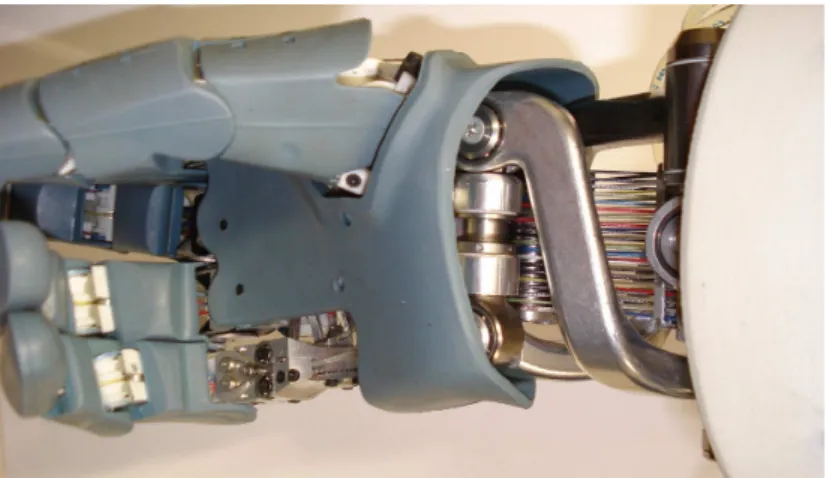
The main reason for the use of tendon, at that time, was that it was impossible to integrate the drives within the hand or in the joints. The advances in mechatronics such as gear box size reduction, power density increase, communication speed increase and, generally, increased availabilty of computation power allowed to build modular hands that integrate the whole drive system within the hand, e. g. the DLR Hand II [22] and the TwendyOne hand [16]. More recently, the Dexhand, an outer space qualiﬁ-able dexterous hand was presented (cf. Fig. 1.10, [23,24]). The drives of the Dexhand are in the palm and the power and control systems are housed in the wrist. However, despite the progress of mechatronics, the size of those robotic hands is still larger than their human counterpart. In order to reach human like ﬁngertip force and maintain a short wrist (that improves manip-ulability), the 38 drives of the hand of the Hand Arm System are located in the forearm.

The Robonaut R2 also contains serial elastic actuators. Furthermore, it is equipped with dexterous hands that are remotely actuated in the forearm [14]. The hands of the Obrero robot are using low mechanical impedance and serial elastic actuators to detect contact and conform to the grasped objects. The hands of the iCub are smaller than human hands and tendon driven. It is a completely open source platform created at the Italian Institute of Technology (IIT).

The humanoid Kenta with a tendon driven spine was developed to be more human like than other humanoids [25] and more recently the robot Kojiro was built that consists of 109 tendon drives (cf. Fig. 1.11, [26]). Un-deractuation is primarily studied in the ﬁeld of robotic protestics. Indeed, the limited control input and the maximum allowed weight leads to a re-duction of the number of actuators. Systems like the cyberhand [27] or the Ottobock prosthesis [28] have been designed to be robust and used easily by the amputee while providing appropriate cosmetic appearance.

Beside these humanoid systems, bio-inspired robotic hands replicating the anatomy of the human hand have been proposed. The anatomically

(35)

Figure 1.11: Kojiro

correct testbed (ACT) Hand [29] and the Shadowhand [30, 31] are both tendon driven hands. The ACT Hand focuses on the one-to-one copy of the human tendon kinematics. The Shadowhand is based on either pneumatic muscles or DC motors. Both are driven by an external actuation unit, not integrated in a hand-arm system. They both have a limited maximum ﬁngertip force and remain fragile w. r. t. impacts.

The kinematic structure is the most important design choice and one of the key challenges in robot hand design. A large number of kinematics, mainly based on empirical results, can be found. They are mostly designed to ﬁt the special needs of existing robot hands like data glove calibration or animation purpose [20].

Alternatively, kinematics can be derived from the analysis of human kinematics. In [32], Giurintano and Hollister developed a ﬁve link kinematics for the thumb based on cadaver analysis to reproduce the motion of the human thumb as close as possible. Stillfried measured the kinematics of a human hand using MRI3 data and segmentation algorithms to extract the bones motions and therefore the hand kinematics. The institute of Ergonomics of the technical university of Munich synthesized a kinematic model of the whole human body to realize the RAMSIS system4.

Optimization is another promising but complex mean to derive hand kinematics. Santos and Valero-Cuevas [33] modeled the kinematics of

Giur-3_{Magnetic Resonance Imaging}

4_{The RAMSIS model is used mainly to realise ergonomic interfaces, e. g. in automobile}

(36)

intano and Hollister using DH-parameters and optimised these using cadaver test data from [32] and Monte Carlo Simulation. They optimised the found kinematics using Markov Chain Monte Carlo Simulation within a space of 50 parameters [34].

Once the kinematics is obtained, or during its optimization, it can be evaluated by using several approaches. Examples of such methods are:

• mathematical criteria – manipulability ellipsoids [35, 36] – dexterous workspace [37] – grasp stability [38] • evaluation tools – graps planners – experiments

Miller and Allen developed a complete simulation environment : GraspIt! It can, among other things, simulate hands in contact situations and determine grasp quality indices [39]. A motion planning software developed by Rosen Diankov [40] provides a number of metrics calculation that can be used to rank the grasps. Thus, used on a large number of grasps, can be indirectly used to evaluate the quality of the kinematics.

Figure 1.12: Workspace analysis for the thumb of the hand of the Hand Arm System [41].

1.4.3 Soft robotics

The design of the Hand Arm System is mainly driven by the insight that todays humanoid robot systems are not robust enough to be operated in unstructured environments, where collisions cannot be avoided. This lack

(37)

Figure 1.13: Simulation tool for grasp evaluation: GraspIt!

of robustness slows down the development of applications in particular us-ing methods that require unsuccessful tasks such as reinforcement learnus-ing. Therefore, it seems that

future robotic systems have to be able to store energy to meet these requirements [42].

In the recent years a lively discussion about the motivation of variable stiﬀness robots has been led debating their advantages and disadvantages with respect to human interactions and especially safety (e. g. STIFF and THE European projects).

In the design of serial elastic actuators the trade-off between robust-ness/mechanical compliance and task performance/mechanical stiffness has to be fixed. In order to postpone this decision, variable stiffness actuators have been proposed [43–49]. More recently, a European project VIACTORS was conducted to evaluate the state of the art concerning the variable stiff-ness actuators. A valuable output of this project was the definition of a specification datasheet for variable stiffness mechanisms (cf. Fig. 1.14).

Using the speciﬁcation sheets of the mechanisms it is possible to compare, at least globally, the mechanisms. A few of those mechanisms are depicted in Fig. 1.15a, Fig. 1.15b, Fig. 1.15, Fig. 1.16a , and Fig. 1.16b.

Control This section gives an overview of the work done in the last decades in terms of control for nonlinear ﬂexible joints. The references are organized in the same order as the control sections.

The use of tendons to actuate the fingers has a number of advantages. However, because tendons can only pull, it is critical to maintain a mini-mum pulling force on all tendons to avoid issues related to tendon slack. Early work on tendon driven mechanism was introduced in the field of ma-nipulation [50] and formalized by Kobayashi [18]. He proposed a number of definitions for the properties of tendon driven systems, such as tendon controllability and tendon redundancy. In [51], tendon driven mechanisms are studied with the help of oriented graphs.

More recently, in the context of the development of the Hand Arm Sys-tem, work on the stiﬀness and torque workspace of tendon driven

(38)

mecha-FAS A flexible Antagonistic spring element

Antagonistic finger joint

Operating Data

# (quantity) (unit) (value)

Mechanical

1 Continuous Output Power [W] 67,2

2 Nominal Torque [Nm] 2,2

3 Nominal Speed [rad/s] 16,74

4 Nominal Stiffness Variation Time

with no load [ms] 29

5 with nominal torque [ms] 29

6 Peak (Maximum) Torque [Nm] 4,9

7 Maximum Speed [rad/s] 152

8 Maximum Stiffness [Nm/rad] 36

9 Minimum Stiffness [Nm/rad] 1,8

10 Maximum Elastic Energy [J] 0,22

11 Maximum Torque Hysteresis [%] 20

12

Maximum deflection with max. stiffness [°] 1,5

13 with min. stiffness [°] 30

14 Active Rotation Angle [°] 150

15 Angular Resolution [''] 3,1

16 Weight [Kg] 3,9

Electrical

17 Nominal Voltage [V] 24

18 Nominal Current [A] 3

19 Maximum Current [A] 7

Control

20 Voltage Supply [V] 24

21 Nominal Current [A] 0,1

22 I/O protocol [] Biss

Spacewire Coaxial Supply 24 V Watercooling tubes

Figure 1.14: Datasheet format created in the VIACTOR project. Example of the tendon mechanism used in the hand of the Hand Arm System (FAS).

nism with nonlinear flexible elements was presented in [41]. Similar work on the achievable Cartesian stiffness of flexible joint robot is found in [52]. In [53, 54], it is shown that the tendon force distribution problem can be simplified if the tendon stiffness is linear in the tendon force. In [55], ex-perimental work on the implementation of the tendon force distribution algorithm was reported.

In case of small size robots, the friction plays an important role. Un-fortunaly, due to the system size and low serie production, the accurate identification of friction is not a simple task. A complete parameter identi-fication method developed for the LWR (Light-Weight Robot) is presented in [56]. Offline identification methods are time consuming and, often, re-quire assumptions on the friction model [57]. If link side torque sensing is available, it is possible to build an online stiffness observer [58]. Moreover, it is shown in [59] that the joint stiffness can be estimated online.

(39)

(a) FSJ (b) FAS

Figure 1.15: VSA-HD.

(40)

When considering flexibility in robots, two main branches are consid-ered. Flexible link control, where the links themselves are flexing under external loads such as gravity, and flexible joint control, where the links are rigid and the joints have a flexible behavior. Most of the publications about flexible joint control deal with flexibility introduced by the drive train. Consequently, most of the papers are stiffness/inertia ratios that are several orders of magnitude higher than in the case of the Hand Arm System. When the joint deflection of a robot due to its own weigth is large, the local ap-proximation of the Jacobian are not valid and it becomes challenging to derive global controllers [60]. The, usually simple, gravity compensation is not neccessarily simple since the joint stiffness needs to fullfill new condi-tions [61, 62] (intuitively, the stiffness should be stronger that the gravity field). The design of traking controller for flexible joint robots has been reported in [63, 64]. The application of flexible joint control to the active damping of an light weight robot is reported by A. Albu Schäffer in [65, 66]. Extensive work on the impedance control of redundant flexible joint robot has been done by Ott in [67, 68]. Between 1990 and 2000, passiv-ity based control of flexible joint system was considered in [69, 70] as well as for a more general class of systems [71–73]. Passivity based control is ap-plied to hand control in [74], and to telemanipulation in [72,75,76]. Damping control for highly flexible robots is considered in [77], where a feedback is used to decouple the dynamics by double diagonalization, compute a proper damping with a pole identification method and apply the controller in the original coordinates.

Impedance control [78] and admittance control [79] have both been ap-plied to tendon control systems. The goal is usually to provide compliance to help in case of inaccuracies in the models or in the sensors. Controllers are used to provide a tendon compliance or to provide a link compliance. In both cases the sensing of the tendon force is required. The Robonaut research group has published serveral papers on the control of the, not an-tagonistically, tendon driven ﬁngers [80, 81]. Control of a joint driven by antagonistic tendon is presented in [82]. Work on the modeling and control of the hand of the University of Bologna is reported in [83].

Several nonlinear control methods have been applied to the control of flexible joint control. Examples of such methods are: feedback linearization, Lyapunov redesign, backstepping or sliding mode control. This thesis uses the backstepping method as described in [84, p.489]. In [68,85], the method is applied to flexible joint control, however limited to the case of linear stiffness and non-antagonistic actuator configurations.

Generally, optimal control method are challenging to implement in real-time, unless closed form solution can be obtained (e. g. optimality of the bang-bang control for some problems [86]). Direct methods to solve the optimal control problem are reported as early as 1960 (cf. [87]). It has been applied to a very large variety of oﬄine optimization problem such as space

(41)

shuttle trajectory, ship maneuver or throwing problem [88]. However, expect for simple cases, the equations can not be solved analytically and do not give any further insight on the required inputs. Numerical methods are required to construct solutions. Unfortunatly, they require forward and backward integrations and are generally extremely expensive to compute.

An intermediate way between the linear optimal control (Riccati equa-tions) and the optimal nonlinear control (HBJ equaequa-tions), has been proposed around 1962 by Pearson [89] under the name of State Dependant Riccati Equation (SDRE). It has been expanded by Wernly [90] and popularized by Cloutier [91–95]. The method is an intuitive extension of the Algebraic Riccati Equation, applied to a pointwize linearized system. Existance of a SDRE stabilizing feedback is discussed in [96]. The method oﬀers only lim-ited theoretical results for global stability (an excellent survey is provided in [97]) but proved to be eﬀective in practice.

1.5 Organization of the work

The Hand Arm System is a major development achieved by a team of about 20 persons. Thus, parts of the system have been presented in diﬀerent conferences and journals [1, 3, 98]. The work of this thesis is divided into two main parts: the modeling and the control. Figure 1.16 depicts the organization of the works and the logical links between the diﬀerent chapters.

1.5.1 Modeling

The modeling part intends to present the hand of the Hand Arm System in details and constructs, step by step, a kinematic and a dynamic model of the motors, the tendons, the springs, the ﬁngers and the wrist. It follows a bottom up approach and thus starts with the motors.

First, a motor model is proposed and verified with a set of identification experiments. Due to their very small size and their high gear ratio, the motors have significant friction. The identification and compensation of the frictional effect is proposed and experimentally verified.

Next, the tendon actuation and the nonlinear spring elements are in-troduced. The nonlinear spring mechanism is modeled and, similar to the motor modeling, a set of simulations and experiments are carried out to verify its validity. Because the tendon force measurements are performed into the forearm, the friction introduced by the guidings from the fingers to the spring mechanisms is critical. A deep understanding of the friction behavior is paramount to the proper operation of the fingers. Therefore, a set of measurements with different pulley materials, grove shapes, tendon material and sliding surfaces is performed in order to establish a model. Al-though the system is already built, the precise knowledge of the influence of the different parameters allows to verify the calculated values. The results

(42)

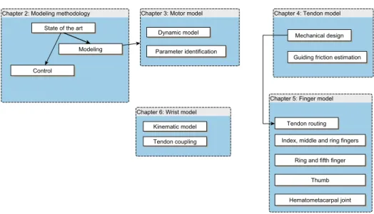
Part I: Modeling and identification

Chapter 2: Modeling methodology

Modeling State of the art

Control

Chapter 3: Motor model

Dynamic model

Parameter identification

Chapter 4: Tendon model

Mechanical design

Guiding friction estimation

Chapter 5: Finger model

Tendon routing Index, middle and ring fingers

Ring and fifth finger

Thumb

Hematometacarpal joint Chapter 6: Wrist model

Kinematic model Tendon coupling

Part II: Control

Chapter 11: Two time scale approach

Controller design

Stability analysis

Experimental results Chapter 10: Tendon control

Model and Controller Gain scheduling Experiments and simulations

Chapter 9: Joint torque observer Structure Experimental setup Experiments and simulations

Chapter 12: Direct pole placement Introduction

Fourth order model Robustness

Chapter 13: Optimal control

Introduction

Fourth order model

Robustness

Chapter 14: State-dependant Ricatti Equation

Introduction Fourth order model

Robustness

Chapter 15: Backstepping

Concept

Single flexible joint: position controller Single flexible joint: impedance

Single flexible joint: impedance nonlinear stiffness

Antagonistic joint

Chapter 16: Optimal backstepping

State-feeedback transformation Optimal problem formulation

Solution

Experiments Simulation

Discussion Chapter 7: Tendon force distribution

Problem formulation Solutions Discussion

Chapter 8: Stiffness correction Model and Controller

Gain scheduling Experiments and simulations

Chapter 17: Conclusion

- The selected hierarchical approach results in a structured model that captures the system behavior

- Several linear and nonlinear control laws are adapted to the specificities of an antagonistic actuation with flexible tendons - Experiements and simulations reveals that nonlinear control approaches are outperforming the linear approaches - The backstepping controller demonstrated on a single joint is applied to the complete hand and is used daily Chapter 1: Introduction

Motivation

- The Awiwi hand : the hand of the Hand Arm System has high dexterity and dynamics - The modeling of the system is required to layout the control structure - We shall investigate the performance of nonlinear control method w.r.t linear approaches

(43)

are a very important tool for the mechanical designers that are seeking a continuous improvement of the system.

The kinematics and the dynamics of the fingers are similar to the case of a serial robot. The kinematics of the finger actuation, from the motor displacements to the fingertip frames are derived using homogeneous trans-formations. The Lagrange and the Newton-Euler methods are presented. A short discussion of their respective strength is given. Simulations are performed to highlight the fact that the Coriolis and centrifugal effects are negligible (at the considered speeds). It does confirm that the governing factor is the mass matrix. The fingers are moved by moving the tendons. Therefore, it is necessary to establish the relationship between the motor motion and the joint motion. The specificities of each fingers are treated in dedicated sections. The fingers have no electronics or cables, conferring them an impressive robustness, it implies however that the link position must be estimated. In the case of the finger, a possible solution is to use a pseudo inverse of the coupling matrix. The thumb actuation is using a tensegrity structure (uncommon for robotic hands) that provides good strength and range of motion. However, because of its nonlinear geometry it implies that the relationship between displacement of the motors and displacement of the link is position dependent. A numerical algorithm is developed and evaluated to estimate, in real-time, the link position. Finally, the ability to adjust the stiffness is studied. The analysis reveals that the stiffness trans-formation between the tendons and the links is obtained with the coupling matrix. The position dependency of the thumb coupling matrix implies that the derivative of the coupling matrix influences the joint stiffness.

All tendons must cross the wrist to go from the motors to the finger inser-tion points. By doing so, a coupling between the wrist moinser-tion and the ten-don displacement is introduced. Although negligible in the flexion/extension direction, the effect is major during the abduction/adduction motions (side-way motions). Consequently, the guidance through the wrist is modeled and included in the kinematic chain of the tendons. The wrist mechanism itself is a double inverted parallelogram and its kinematic modeling is explained step by step. Experiments and simulations are compared and confirm the validity of the model.

1.5.2 Control

The control of robots with a high number of degree of freedom and non-linear components is a globally unsolved problem. Although non-linear control methods have been successfully applied on slightly nonlinear system, highly nonlinear plants remain diﬃcult to control. In the control part, the chal-lenges related to the tendon actuation and elastic joint control are treated. Approaches from the linear control theory as well as the nonlinear control theory are used. Since the Hand Arm System is an important research