HAL Id: hal-00759865
https://hal.archives-ouvertes.fr/hal-00759865
Submitted on 3 Dec 2012
HAL is a multi-disciplinary open access
archive for the deposit and dissemination of
sci-entific research documents, whether they are
pub-lished or not. The documents may come from
teaching and research institutions in France or
abroad, or from public or private research centers.
L’archive ouverte pluridisciplinaire HAL, est
destinée au dépôt et à la diffusion de documents
scientifiques de niveau recherche, publiés ou non,
émanant des établissements d’enseignement et de
recherche français ou étrangers, des laboratoires
publics ou privés.
STABILITY OF MANIPULATOR CONFIGURATION
UNDER EXTERNAL LOADING
Alexandr Klimchik, Anatol Pashkevich, Damien Chablat
To cite this version:
Alexandr Klimchik, Anatol Pashkevich, Damien Chablat. STABILITY OF MANIPULATOR
CON-FIGURATION UNDER EXTERNAL LOADING. Proceedings of the 11th Biennial Conference on
Engineering Systems Design and Analysis, Jul 2012, Nantes, France. pp.1-10. �hal-00759865�
Proceedings of the 11th Biennial Conference on Engineering Systems Design and Analysis ESDA2012 July 2-4, 2012, Nantes, France
ESDA2012-82217
STABILITY OF MANIPULATOR CONFIGURATION UNDER EXTERNAL LOADING
Alexandr Klimchika,b, Anatol Pashkevicha,b, Damien Chablatba
Ecole des Mines de Nantes, 4 rue Alfred-Kastler, 44307 Nantes, France
b
Institut de Recherches en Communications et Cybernétique de Nantes, UMR CNRS 6597, France
KEYWORDS
Parallel robots, stiffness modeling, equilibrium stability, elastostatic singularity.
ABSTRACT
The paper is devoted to the analysis of robotic manipulator behavior under internal and external loadings. The main contributions are in the area of stability analysis of manipulator configurations corresponding to the loaded static equilibrium. In contrast to other works, in addition to usually studied the end-platform behavior with respect to the disturbance forces, the problem of configuration stability for each kinematic chain is considered. The proposed approach extends the classical notion of the stability for the static equilibrium configuration that is completely defined the properties of the Cartesian stiffness matrix only. The advantages and practical significance of the proposed approach are illustrated by several examples that deal with serial kinematic chains and parallel manipulators. It is shown that under the loading the manipulator workspace may include some specific points that are referred to as elastostatic singularities where the chain configurations become unstable.
1. INTRODUCTION
Manipulator stiffness modeling under loading is a relatively new research area that is important both for serial and parallel robots. In general case, loadings may be of different nature and applied to different points/surfaces. To evaluate stiffness properties, several methods can be applied such as Finite Element Analysis, Matrix Structural Analysis and Virtual Joint Modeling (VJM) [1-16], where the last one is the most attractive in robotic domain since it operates with an extension of the traditional rigid model that is completed by a set of virtual joints (localized springs), which describe elastic properties of the links, joints and actuators.
For serial manipulators the VJM approach has been used in the number of works [1-8]. The obtained results allows us to compute stiffness matrices both for serial manipulators without passive joints [1-5] and for serial chains of parallel manipulators with passive joints [8]. However, most of them addressed to the case of small deflections (unloaded mode) [5-6], only limited number of authors consider the case of large deflections (loaded mode) [2-3,7-8].
For parallel manipulators, the stiffness modeling is usually performed for all kinematic chains simultaneously [6][11], using the aggregated elastostatic equilibrium equations [12][13]. In contrast to these works, our approach is based on two-step procedure, which includes stiffness modeling of all kinematic chains separately and then aggregates them in a unique model. This approach has been already used by several authors [8][14], but related aggregation technique was reduced to simple summations of the Cartesian stiffness matrices for the kinematic chains and the external loadings applied to their end-points. This corresponds to “pure” parallel architectures where the end-point location of all kinematic chains are aligned and matched at the end-platform reference point. However, in practice, the parallel manipulator architecture is usually quite complex. In particular, the kinematic chains may be attached to different points of the end-platform.
It is obvious that the both external and internal loadings influence on the manipulator equilibrium configuration and, consequently, may modify the stiffness properties. So, they must be undoubtedly taken into account while developing the stiffness model. However, in most of related works the stiffness is evaluated in a quasi-static configuration without external or internal loading. There are very limited number of publications that directly address the case of “large deflections”, where in addition to the conventional “elastic stiffness” in the joints it is necessary to take into account the “geometrical stiffness” arising due to the change in the manipulator configuration under the load. The most essential results in this area were obtained in
[7-10,14] where there are presented both some theoretical issues and several case studies for serial and parallel manipulators under end-point loading. Several authors [9,13] addressed the problem of stiffness analysis for the manipulators with internal preloading or antagonistic actuating, but in relevant equations some of the second order kinematic derivates were neglected. However, no one of them considered auxiliary loading.
This paper contributes to the VJM-based technique and focuses on the stability analysis of serial and parallel manipulators under external loading. It addressed both stability of end-platform location and stability of serial chain configuration. To address these issues, it is proposed a revision of the existing VJM-based stiffness modeling technique that includes development a non-linear stiffness model of the robotic manipulator under essential loading that takes into account the external loading applied to end-effector, preloading in the joints and auxiliary loading applied to intermediate node-points.
2. PROBLEM STATEMENT
2.1 Motivation
Traditionally, the stability of compliant mechanical systems (including manipulators) is defined as resistance of the
end-point location t with respect to the “disturbing” effects of an external force F applied at this point. In such formulation, the stability is completely defined by the stiffness matrix KC that
describes the linear relations between the force and deflection deviations δ , δF t with respect to the values F , t.
C
δF K δt (1)
It is obvious that for the stable location t the matrix KC should
be positive definite.
However, in the compliant manipulators with the passive joints, the equilibrium configuration ( , )q θ corresponding to the same end-point location t cannot be unique (here the vector q
contains passive joint coordinates; the vector θ collects coordinates of all virtual joints). Moreover, these configurations may be both “stable” and “unstable” and may correspond to different values of potential energy stored in the virtual springs. From this point of view, it is worth to distinguish stability of the end-point location t and stability of the corresponding equilibrium configuration of the kinematic chain ( , )q θ , which may be defined as a resistance of the chain shape with respect to disturbances in redundant kinematic variables. This issue becomes extremely important for the loaded mode, when due to the kinematic redundancy caused by the passive joints and excessive number of virtual springs, small disturbances in ( , )q θ may provoke essential change of current equilibrium configuration leading to the reduction of the potential energy and transition to another equilibrium state, while keeping the
same end-point location. Hence, it is necessary to evaluate internal properties of the kinematic chain in the state of the loaded equilibrium that may correspond either to minimum or maximum of the potential energy for a fixed value of t.
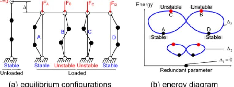
Let us illustrate this notion by the example of three-link chain (Figure 1a), which includes passive joints at both ends and two virtual torsional springs between the links, which insure the "straight" configuration for the unloaded mode. It is assumed that both ends of the chain are fixed by the external geometrical constrains while the internal configuration may change without shifting of the end-points, in accordance with redundant parameter value. It is evident that this chain is loaded, but corresponding value of the force F depends on particular configuration. Besides, among variety of possible configurations (corresponding to given end-point locations), only equilibrium ones are in the focus of interest.
Redundant parameter Energy FC FB FD FA A B C D
(a) equilibrium configurations (b) energy diagram F=0 A D B C Stable Stable Unstable Unstable 1 0 2 3
Stable Unstable Unstable Stable
Unloaded Loaded
Stable
Figure 1 Stable and non-stable configurations of 3-link serial chain and their energy-based interpretation
For this case study, it is convenient to give an energy-based interpretation. The considered kinematic chain has one redundant parameter (rotation angle of any passive joint) and under geometrical constrains may occupy configurations with the different shapes. Relevant relation between the energy stored in the virtual springs and the redundant parameter value is presented in Figure 1b. Due to the physical nature of this chain, for each given end-point displacement , the examined plot presents a continuous closed criss-cross curve that has exactly two minimum and maximum points, that correspond to the stable and unstable equilibriums respectively. Hence, numerical solution of static equilibrium equations may yield both stable and unstable configurations, while in practice only stable ones should be considered. Thus, the criterion that allows to distinguish stable and unstable configurations of the kinematic chain is required.
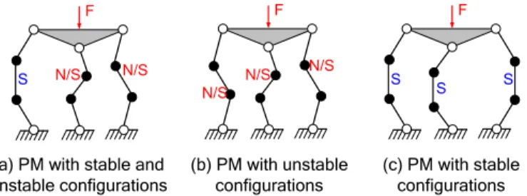
Physical meaning of this stability notion (related to the kinematic chain shape) is illustrated in Figure 2, which contains several postures of the same parallel manipulator with exactly the same end-platform location. These postures differ in the shapes of serial kinematic chains that may be treated as internal configuration of the parallel manipulator, which is not "visible" from the end-platform side whose static stability is completely defined by the Cartesian stiffness matrix. In particular, Figure 2a,b present parallel manipulators that include at least one
kinematic chain in unstable configuration that cannot be observed in practice but satisfy the general static equilibrium equation. In contrast, Figure 2c shows physically realizable posture of the same manipulator (with exactly the same location of the chain end-points) where for all kinematic chains the shapes are stable.
(b) PM with unstable
configurations (c) PM with stable configurations
F
(a) PM with stable and unstable configurations F F S N/S N/S N/S S S N/S N/S S
Figure 2 2D parallel manipulators with serial chains in stable and unstable configurations
Hence, full-scale investigation of the stiffness properties of the loaded parallel manipulator must include the stability analysis of the internal kinematic chain configurations that is presented in this paper.
2.2 Basic assumptions and research problems
In order to address the stability of both end-point location and kinematic chain configuration, it is assumed that parallel manipulator has a strictly parallel structure. In this case, first, it is required to address to the stiffness modeling of serial kinematic chain and then, applying stiffness model aggregation technique, to obtain the stiffness matrix of the parallel manipulator.
...
Ps Ps
Link
Ac Rigid Link Link Ps
Link 6-d.o.f. spring 6-d.o.f. spring 6-d.o.f. spring F Gn G2 G1
Figure 3 VJM model of kinematic chain with end-point and auxiliary loading
For stiffness modeling of serial kinematic chain let us use VJM model that is presented in Figure 3. It is assumed that, in addition to the end-point loading F the serial chain has an additional external loadings applied to the internal node points (auxiliary loading). These forces will be denoted as Gj, where
1, ...,
j n is the node number in the serial chain starting from the fix base. For such kinematic chains it is necessary to introduce the functions defining locations of the nodes
( , ), 1, ...,
j j j n
t g q θ (2)
where the vector tj includes the position and orientation of the
ith node; the vector q contains passive joint coordinates; the vector θ collects coordinates of all virtual joints.
Using these assumptions and the methodology of VJM method proposed in [8][10], the problem of stability analysis of serial and parallel manipulators under external/internal loading can be split in the following sub-problems: (i) stability analysis of serial chain configuration that includes computing of the loaded equilibrium configuration, and (ii) stability of the end-okatform location of serial and parallel manipulators.
3. STABILITY OF KINEMATIC CHAIN CONFIGURATION UNDER LOADING
Usually external and internal loadings have affects both end-point location and configuration of serial chain. Therefore, in order to address to the stability of the kinematic chain configuration; firstly; it is required to compute the loaded equilibrium configuration.
3.1 Static equilibrium
The static equilibrium equations for the manipulators with internal and external loadings (that are applied to both end-effector and intermediate nodes) differ from those used for the end-point loaded manipulator. Using the principle of virtual work it has been proved that the desired static equilibrium equations can be presented as
(G ) T (F ) T 0 θ θ θ (G ) T (F ) T q q J G J F K θ θ J G J F 0 (3) where (F) ( ) ( ) ( ) (G ) (1) ( ) θ θ q q θ θ θ (G ) (1) T T T T T T ( )T T T q q q 1 ; ; ... ; ... ; ... n F n n n n J J J J J J J J J J G G G (4)and Jacobians with respect to the virtual and passive joint coordinates respectively can be computed as
( ) ( ) θ , ; q , j j j j J g q θ J g q θ θ q (5)To obtain a relation between the external loading F and internal coordinates of the kinematic chain ( , )q θ
corresponding to the static equilibrium, Eq. (3) should be solved either for given values of F or for different given values of t. In [10] these problems were referred to as the original and the dual ones respectively, but the dual problem was discovered to be the most convenient from computational point of view. Hence, let us solve static equilibrium equations with respect to manipulator configuration
q θ,
and external loading F for given end-effector position tg q θ
,
and function of auxiliary-loadings G q θ
,
Since usually this system has no analytical solution, iterative numerical technique can be applied. For this purpose,
the kinematic equations may be linearized in the neighborhood of the current configuration (qi,θi)
(F) θ (F 1 q 1 1 ) , , , ; i i i i i i i i i i i t g q θ J q θ θ θ J q θ q q (6)where the subscript "i" denotes the iteration number and the changes in Jacobians (G ) (F) (G ) (F)
θ , θ , q , q
J J J J and variation of the auxiliary loadings G q θ
,
from iteration to iteration are assumed to be negligible. Correspondingly, the static equilibrium equations in the neighborhood of (qi,θi) may be rewritten as
(G ) T (F ) T 0 θ θ θ (G ) T (F ) T q 1 q 1 1 i i i J G J F K θ θ J G J F 0 . (7)Thus, combining Eq. (6) and (7), the iterative algorithm for computing the static equilibrium configuration for given end-effector location can be presented as
1 (F ) (F ) q θ (F ) T (G ) T q q (F ) T (G ) T 0 θ θ θ θ (F ) (F 1 1 1 ) q 1 , θ · i i i i i i i i i i 0 J J ε F q J 0 0 J G θ J 0 K J G K θ ε t g q θ J θ J q (8) where Gi1G q( i1,θi1).The proposed algorithm allows us to compute the static equilibrium configuration for the serial chains with passive joints and all types of loadings (internal preloading, external loadings applied to any point of the manipulator and loading from the technological process). The convergence properties of this algorithm are similar to one presented in [10]. Also, it can be modified to solve the problem of computing the equilibrium configuration corresponding to given external loading.
3.2 Stability criterion
To evaluate stability of the static equilibrium configuration ( ,q θ) of a separate kinematic chain, let us assume that the end-point is fixed at the end-point T
( , )
t p φ corresponding to the external load F , but the joint coordinates are given small virtual displacements q, θ satisfying the geometrical constraint (2), i.e.
( , ); ( δ , δ )
t g q θ t g q q θ θ (9)
For these assumptions, let us compute the total virtual work in the joints that must be positive for a stable equilibrium and negative for an unstable one. To achieve the virtual configuration (qδ ,q θδ )θ and restore the equilibrium conditions, each joint must include a virtual spring that
generates the generalized forces/torques δτq, δτθ which
satisfies the equations:
T T θ θ 0 ; q 0 J F K θ θ J F (10) T θ θ θ 0 θ T q q ( δ ) ( ) δ ( δ ) δ q J J F K θ θ θ τ J J F τ (11)After relevant transformations, the virtual torques may be expressed as
T T
θ θ θ q q
δτ δ(J F)K δ ;θ δτ δ(J F) (12) where δ (...) denotes the differential with respect to δ q, δθ that may be expanded via Hessians of the scalar function
T ( , ) g q θ F: T F F θ θq θθ T F F q qq qθ δ( ) δ δ δ( ) δ δ J F H q H θ J F H q H θ (13) provided that F 2 2 F 2 2 qq θθ F F 2 qθ θq T / ; / ; / H q H θ H H q θ (14)
Further, taking into account that the virtual displacement from ( ,q θ) to (qδ ,q θδ )θ leads to a gradual change of the torques in the virtual joints from (0, 0) to (δτq, δτθ), the virtual
work may be computed as a half of the corresponding scalar products
T T
θ q 1 δ δ δ δ δ 2 W τ θ τ q (15) where the minus sign takes into account the adopted conventions for the positive directions of the forces and displacements. Hence, after appropriate substitutions and transformations to the matrix form, the desired stability condition may be written asF F θθ θ qθ T T F F θq qq 1 δ δ δ δ 0 δ 2 W H K H θ θ q q H H (16)
where q and θ must satisfy (9).
In order to take into account the relation between δ q and δθ that is imposed by (9), let us apply the first-order expansion of the function g θ q( , ) that yields the following linear relation
θ q δ δ J J θ 0 q (17)
T θ T θ q θ q q r V S J J U U 0 V (18)
and extracting from Vθ, Vq the sub-matrices o θ
V , o
q
V
corresponding to zero singular values, a relevant null-space of the system (17) may be presented as
o o
θ q
δθV δ ;μ δqV δμ (19) where δ μ is the arbitrary vector of the appropriate dimension (equal to the rank-deficiency of the integrated Jacobian
θ q
[J , J ]). Hence, changing of the potential energy δW because of variation of the redundant variables δ μ (16) may be rewritten as T F F o o θθ θ qθ T θ θ o F F o q θq qq q 1 δ δ δ 0 2 W H K H V V μ μ V H H V (20)
that must be satisfied for all arbitrary non-zero δ μ. Hence, the considered static equilibrium configuration ( ,q θ) is stable if (and only if) the matrix
T F F o o θθ θ qθ θ θ o F F o q θq qq q 0 c S H K H V V V H H V (21)
is negative-definite. It is worth mentioning that the obtained result is in a good agreement with the previous studies [4], where (for the manipulators without passive joints) the stiffness properties were defined by the matrix F
θ θθ
K H that evidently must be positive-definite for the stable configurations.
Thus, the proposed stability analysis technique for serial chain with the passive joints and related matrix stability criterion for the kinematic chain configuration allow us to estimate the stability of the serial chain configuration under the external loading in the case of single and multiple equilibriums.
4. STABILITY OF THE END-PLATFORM LOCATION UNDER EXTERNAL LOADING
Similar in the structural mechanics stability of the robot end-platform location is defined by the Cartesian stiffness matrix. However, stiffness matrices of serial and parallel manipulators are computed in a different manner (here, to compute stiffness matrix of parallel manipulator it is required to have stiffness matrices of all its serial chains). Let us address them sequentially.
4.1 Cartesian stiffness matrix of a serial kinematic chain
Following the virtual work technique and using static equilibrium equations (3), force deflection relations for the considered serial chain can be expressed as
(F ) (F ) q θ (F ) T q q q q θ (F ) T θ θq θ θθ δ δ δ δ 0 J J t F 0 J H H q 0 J H K H θ (22)
where Hessians can be computed as
12 1 2 12 1 (F ) (G ) (G ) T v v v v v v v 2 H H H J G v , (23) where (v1,v2){ ( , ), ( , ), ( , ), ( , )}q q q θ θ q θ θ and
12 1 2 T T 1 2 1 2 2 (G ) ( 2 F) v v v v 1 1 ; · · ; n n j j j j
H g G H g F v v v v . (24)Hence, the desired stiffness matrices can be computed via the matrix inversion 1 (F ) (F ) q θ C (F ) T q q q q θ (F ) T θ θq θ θθ * * 0 J J K J H H J H K H (25)
Further, using several analytical transformations and applying the block matrix inversion technique of Frobenius [17], the Cartesian stiffness matrix can be compute as
0 ( ) 0 ( ) F 0 ( ) C q F F F C C C K K K k K (26)
where the first term 0 ( ) F T 1 θ θ θ ( ) F C K J k J exactly corresponds to the classical formula defining stiffness of the kinematic chain without passive joints in the loaded mode, [5], and the second term take into account influence of passive joints via matrix F
q k
1 F F F F 0 ( ) F F q q· qq qθ θ θq q q · q T F C T k J H H k H J K J J (27) here F θk denotes the modified joint compliance matrix
F 1 θ ( θ θθ) k K H and matrix F q
J denotes the modified Jacobian with respect to passive joints F
F
q q θ θ θq
J J J k H .
Thus, the Cartesian stiffness matrix obtained using Eq. (26) allows us to analyze the stability of the serial manipulator (or kinematic chain) end-point location under external/internal loadings. If this stiffness matrix is positive definite the end-point location is stable, and if it is rank-deficient (negative definite) it is possible to move end-point location without additional efforts.
4.2 Cartesian stiffness matrix of parallel manipulator
Let us assume that a parallel manipulator may be presented as a strictly parallel system of the actuated serial legs connecting the base and the end-platform [18]. Using the methodology described in previous sections and applying it to each leg, there can be computed a set of m Cartesian stiffness
matrices ( ) C
i
K expressed with respect to the same coordinate system but corresponding to different platform points (Figure 4). If initially the chain stiffness matrices were computed in local coordinate systems, their transformation is performed in a standard way [19]. 1 v 2 v 3 v (c) (b) 1 v 2 v 3 v 1 u 2 u 1 v 2 v 3 v (a) F M F M MF
Figure 4 Typical parallel manipulator (a) and transformation of its VJM models (b, c)
After such extension, an equivalent stiffness matrix of the leg may be expressed using relevant expression for a usual serial chain, i.e. as ( ) T ( ) ( ) 1
v · C· v
i i i
J K J , where the Jacobian ( ) v
i
J
defines differential relation between the coordinates of the i-th virtual spring and the reference frame of the end-platform. Hence, the final expression for the stiffness matrix of the considered parallel manipulator can be written as
T 1
( ) ( ) ( ) ( ) С v С v 1 · · m m i i i i
K J K J (28)where m is the number of serial kinematic chains in the manipulator architecture.
As a result, Eq. (28) allows us to compute the Cartesian stiffness matrix for the parallel manipulator based on the stiffness matrices for serial chains and transformation Jacobians
( ) v
i
J , which define geometrical mapping between the end-points of serial chains and the reference point frame (the end-effector). Hence, the axes of all virtual springs are parallel to the axes x,
y, z of this system. This allows us to evaluate Jacobians ( ) v
i
J and their inverses from the geometry of end-platform analytically
( ) 3 ( ) 1 3 v v 3 6 6 3 6 6 ( ) ( ) , i i i i I v I v J J 0 I 0 I (29)
where I3 is 33 identity matrix, and
v is askew-symmetric matrix corresponding to the vector v, that defines the end-platform location with respect to the end-point of kinematic chain.
It should be mentioned that the proposed approach is also able to take into account geometry of end-platform and it connection with kinematic chains in an explicit form. Finally, using results of Eq. (28) it is possible to analyze the stability of the end-effector location of the parallel manipulator under external loading.
5. APPLICATION EXAMPLES
5.1 Stiffness analysis for serial chain with 1D-springs
Let us illustrate the efficiency of the developed techniques on the example of 3-link kinematic chain with rigid links and two virtual springs between them. It is assumed that both ends of the chain are fixed with rotational passive joints, all link length are equal to l and the stiffness coefficient of both springs are equal to Kθ. The end-point location of considered serial chain can be expressed using geometrical model as
1 1 2
1 1 2
·cos( ) ·sin( ) ·cos( )
·sin( ) ·sin( ) ·sin( )
x l l l y l l l q q q q q q (30)
where coordinates x y, define end-point location and angle defines its orientation, q and 1, 2 are passive and virtual joint
coordinates respectively that define serial chain configuration. It is assumed that external loading is applied along x-direction only and manipulator end-point can move along x-axis only. So external loading F can be presented as F
F 0
T where Fis applied external loading along x-axis.
Assuming that the initial values of the actuating coordinates (i.e. before the loading) are denoted as 0
1
, 0 2
, the potential energy stored in the virtual springs may be expressed as the following function of the redundant variable
0
2
0
2 θ 1 1 θ 2 2 1 1 ( ) ( ) ( ) 2 · · 2 E q K q K q (31)where Kθ is the stiffness coefficient, and 1, 2 are computed
via the inverse kinematics. Using these equations, the desired equilibriums may be computed from the extremum of E q( ). In particular, stable equilibriums correspond to minima of this function, and unstable ones correspond to maxima.
Figure 5 Energy diagram for 3-link serial chain To illustrate this approach, Figure 5 presents a case study for the initial S-configuration ( 0
0 q , 0 1 0 θ and 0 1 0 θ ). It allows comparing 12 different shapes of the deformated chain and selecting the best /worst cases with respect to the energy. As it follows from these results, here there are two symmetrical maximum and two minimum, i.e. two stable and two unstable equilibriums. Besides, the stable equilibriums correspond to
-shaped deformated postures, and the unstable ones correspond to Z-shaped postures, as it is shown in Figure 6
Figure 6 Evolution of the S-configuration under loading If the assumption concerning small values of is released, analytical solutions for the non-trivial equilibriums may be still derived. In particular, for the stable equilibrium, one can get
θ S( ) sin K F L (32)
where arcco s(1 / 2 ). For the unstable equilibrium similar equation may be written as
θ N co s( ) 2 co s ( ) sin K q q F L (33) where 2 2 1 2 6 3 arcco s ; arcco s 1 1 2 4 2 4 q (34)
Corresponding plots with the bifurcation are presented in Figure 7. The interpretation of this plot is similar to the axial compression of a straight column, which is a classical example in the strength of materials. It should be noted, that the developed numerical algorithm exactly produces the curve corresponding to the stable equilibrium.
Figure 7 Force-deflection relations for S-configuration
Figure 8 Evolution of the Z-configuration under loading
However, for Z-configuration that corresponds to the unloaded zig-zag shape, the stiffness behavior demonstrates the buckling that leads to sudden transformation from a symmetrical to a non-symmetrical posture as shown in Figure 8. Here, there exist two stable equilibriums that differ in the values of the potential energy,
In order to analyze stability of different configurations let us define Jacobians and Hessian matrices. For the considered serial chain Jacobinas can be expressed as
1 1 2 1 2
θ
1 1 2 1 2
sin ( ) sin ( ) sin ( )
· co s( ) co s( ) co s( ) q q q q q q l J (35) and 1 1 2 q 1 1 2
sin ( ) sin ( ) sin ( )
· co s( ) co s( ) co s( ) q q q q q q l J (36) and Hessians as 1 1 2 1 2 θθ 1 2 1 2 ( ) co s( ) co s( ) · co s( ) co s( co s ) q q q l q F q H (37) 1 1 2 θq 1 2 ( ) co s( ) ·· co s co s( ) q q F l q H (38) 1 1 2 qθ 1 2 ( ) cos( ) · · c s cos o ( ) T q q q F l H (39)
qq F· · cos( )l q cos(q1)cos(q12)
H (40)
The eigenvectors for the matrix V that is required in (21) can be obtained from the matrix JT·J, where J [Jθ, Jq],
which for the considered serial chain can be computed from
2 2 2 2 2 2 2 2 3 2 ( ) 2 ( ) · · · 2 ( ) 2 1 ( ) 2 co s co s co s co s co s( ) 1 co s( ) 1 x T l F J J (41)
In order to obtain eigenvalues of (41), it is required to solve the third order equation
3 3 2
2 2
2
2 2
6 ·( cos(6 ) 2) 3cos ( cos co ) 4 ( ) 2 s( ) 1 0 (42) with respect to .
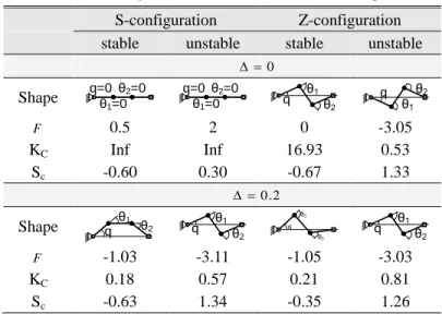
Using the above equations, let us investigate stability of 3-link serial chain using the developed matrix criterion in the S- and Z- configurations (these shapes of the chain correspond to the unloaded configurations). For the Z-configuration the unloaded configuration is defined by the angles 0
9 .9 0
0 1 3 0 θ and 0 1 3 0 θ
that correspond to the end point location x2 .9 1 ;·l y0. Modeling results are presented in Table 1. This table includes the external loadings F that are normalized with respect to Kθ /L, the Cartesian stiffnesses KC
that are also normalized with respect to Kθ /L, and the stability of serial chain configuration Sc (as it was mentioned negative value corresponds to stable configuration and positive to unstable configuration) as well as the shapes of the chains. The results have been obtained for the cases of 0 and 0 .2, here is the normalized the end-point deflection / l, and
is the absolute displacement.
Table 1 Stability of 3-link serial chain under loading S-configuration Z-configuration stable unstable stable unstable
0 Shape q=0θ 1=0 θ2=0 q=0 θ1=0 θ2=0 q θ1θ 2 q θ1 θ2 F 0.5 2 0 -3.05 KC Inf Inf 16.93 0.53 Sc -0.60 0.30 -0.67 1.33 0 .2 Shape q θ1 θ2 q θ1 θ2 q θ1 θ2 q θ1θ 2 F -1.03 -3.11 -1.05 -3.03 KC 0.18 0.57 0.21 0.81 Sc -0.63 1.34 -0.35 1.26
The results show that for the stable configurations the value of Sc is always negative and for the unstable configurations it is positive. Hence, numerical results that have been obtained using the stability criterion (21) are in a good agreement with analytical ones. Moreover, it is shown that for the unstable configuration the stiffness coefficient KC is positive and,
consequently, it cannot be used for the stability analysis of kinematic chain configuration.
5.2 Stability of serial chain under auxiliary loading
Let us now focus on the stability analysis of a serial chain under auxiliary loadings applied to an intermediate node. It is assumes that the considered chain consists of two rigid links separated by a flexible joint and two passive joints at both ends. It is assumed that the left passive joint is fixed with a physical constraint, while the right one is balanced by external loading
x
F and can be moved along x direction (Figure 9). Besides, here both rigid links have the same length L and the actuator stiffness is Kθ.
Let us assume that the initial configuration (i.e. for 0
M ) of the manipulator corresponds to 0 / 6, where
2·
is the coordinate of the actuated joint, is the angle
between the first link and x-direction. It is also assumed that the external loading G is applied to the intermediate nod (Figure 9) and it is required to apply the external loading (Fx,Fy) at the end-point to compensate the auxiliary loading
G. Since this example is quite simple, it is possible to obtain the force-deflection relation and the stiffness coefficient analytically. The force-displacement relation and the stiffness can be expressed in a parametric form as
θ 0 co s · 2· · ; 2 sin sin 2 x y K G G F F L (43)
θ 3 3 0 2 ·co s sin 1 · · 4 sin sin x K G K L L (44)where ( / 2; / 2 ) is treated as a parameter, Ky 0. As it follows from expression (44), the stiffness coefficient x
K essentially depends on the auxiliary loading G , coefficient x
K can be both positive and negative or even equal to zero when the auxiliary loading is equal to its critical value
θ *
0
4 / ·sin
G K L . It is evident that the case *
G G is very dangerous from practical point of view, since the chain configuration is unstable.
The force-deflection relations and values of translational stiffness Kx are presented in Figure 10. They show that the auxiliary loading G significantly reduces the stiffness of the serial chain. Further increasing of the auxiliary loading up to
*
1.5·
G G leads to the unstable configuration with negative stiffness 2 θ 7 .4 6 ·K /L . G Fx L L θ K y x Fy
Figure 9 Kinematic chain with compliant actuator between two links and its static forces
Figure 10 Force-deflections relations for different values of
auxiliary loading G ( * θ 0 4 / ·sin G K L , 2 θ · / x K K K L )
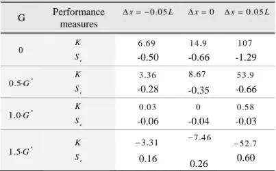
Table 2 Translational stiffness 2 θ / · x K K L K and stability coefficients Sc for different values of auxiliary loading G and different displacements x ( * 0 4 / ·sin G K L ) G Performance measures 0.05 x L x 0 x 0 .0 5L 0 K c S 6.69 -0.50 14.9 -0.66 1 0 7 -1.29 * 0.5·G K c S 3.36 -0.28 8.67 -0.35 53.9 -0.66 * 1.0·G K c S 0.03 -0.06 0 -0.04 0.58 -0.03 * 1.5·G K c S 3.31 0.16 7 .4 6 0.26 5 2 .7 0.60 To investigate the stability of serial chain configuration and the stability of the end-point location additional, analysis have been performed. Simulation results are summarized in Table 2 that contains both translational stiffness 2
θ
/ ·
x
K K L K and stability coefficients δW for different values of auxiliary loading G and displacements x. The results confirm that when auxiliary loading G overcomes it critical value *
G both configuration and the end-point location of serial chain become unstable. Hence, the presented case study demonstrates rather interesting features of stiffness behavior for kinematic chains under auxiliary loading that where not studied before (negative stiffness, non-monotonic force-deflection curves, etc.).
5.3 Kinetostatic singularity in the neighborhood of the flat configuration
Let us consider now an example that deals with the stability analysis of Orthoglide manipulator (Figure 11a). Detailed specification of this manipulator can be found in [20], some results on the stiffness analysis have been presented in [8][10]. In this case study let us address the stiffness analysis (which includes stability analysis of end-point location under external loading) of Orthoglide manipulator in the neighborhood of a flat configuration. Simulation results for this posture are presented in Figure 11b and Table 3 where d0 denotes the initial distance
from the flat singularity, K0 is the translational stiffness for the
unloaded mode, (cr ,Fcr) and (cr,Fcr) are respectively the critical deflection and the critical force for the opposite directions of the displacement. As it follows from these results, in the neighborhood of the flat singularity the stiffness properties are essentially non-symmetrical with respect to the force direction. In particular, for the inside-direction of the loading, the force increases non-linearly but monotonically while the deflection augments. However, for the outside-direction, initially the manipulator reacts to the external loading in the same way: increasing of the deflection leads to increasing of the resisting elastic force. But after achieving the critical
value, the reacting force begins decrease, the configuration becomes unstable and the manipulator abruptly changes its posture to the symmetrical ones. After that, the manipulator demonstrates stable behavior with respect to the loading.
(b) force-deflection relation -20 -10 0 -20 -10 0 10 20 30 40 , mm , F N buckling 0 11.4 d mm Fcr»11.1 N Q1 Q2 Q0 Q3 Q4
(a) Orthoglide manipulator
Figure 11 Force-displacement relations for Orthoglide
manipulators (distance to the singularity is 11.4 mm)
Table 3 Summary of stiffness analysis in the neighborhood of the flat singularity
Configuration d0, [mm] c r F, [kN] cr , [mm] c r F, [kN] cr , [mm] Point Q2 91.7 -2.06 -5.7 2.20 4.9 Point Q2a 46.0 -0.70 -17.1 1.45 11 Point Q2b 11.4 -0.01 -4.6 0.92 24 Q2 = (-76.35, -76.35, -76.35); Q2a = (-100, -100, -100); Q2b = (-120, -120, -120)
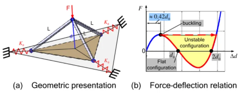
The simplest model that explains the above described phenomenon is presented in Figure 12. It is derived via generalization of the “toggle-frame” construction, with relevant modifications motivated by the Orthoglide architecture and relative stiffness properties of its elements. Here, the elasticity is concentrated at the basis of the manipulator legs and it is presented by linear springs with the parameter K. It is assumed that initial distance between the end-point and the singularity-plane is d0 Lsin0, where 0 is corresponding
angle between the leg and the plane. The derived expressions
0 0 0 0 3 1 co s / co s sin ; sin sin F K L d L (45)perfectly describe the shape of the force-deflection curves obtained from the complete stiffness models.
Besides, more detailed analysis shows extremely fast reduction of the stiffness while approaching this singularity. Corresponding expressions derived for small value of 0 yield
a linear relation for the critical deflection cr 0 .4 2d0 and
cubic relation for the critical force 2 3 0
/ 3
cr
F K L d . Hence,
this simplified model is in good agreement with the simulation results and justifies conventional kinematic design objectives (velocity transmission factors, condition number, etc.) that preserve the manipulator from approaching the flat posture.
F d L L L K K K
(a) Geometric presentation (b) Force–deflection relation 0 F d Unstable configuration Flat configuration buckling 0 0.42d 0 d 0 2d
Figure 12 Simplified stiffness model of Orthoglide-type manipulators for near-flat configuration
Hence, the considered example illustrates the ability of proposed technique to obtain the full-scale force-deflection relation for the parallel manipulators that is suitable for the stability analysis of end-point location under the external loading. It proves that the common notion of the “distance-to-singularity” that is used in kinematics must be revised in elastostatics taking into account that loading essentially reduces the margin of the manipulator structural stability.
6. CONCLUSIONS
The paper presents new approach for the stability analysis of parallel manipulators under internal and external loadings applied to different points. In contrast to other works, it is proposed to address both stability of the end-effector location and stability of kinematic chain configuration. This approach is based on the non-linear stiffness analysis that includes computing the static equilibrium configuration corresponding to the given loadings as well as computing the Cartesian stiffness matrices for serial chains and parallel manipulators. The advantages of the proposed approach are illustrated by several examples
ACKNOWLEDGMENTS
The work presented in this paper was partially funded by the Region “Pays de la Loire”, France and by the project ANR COROUSSO, France.
REFERENCES
[1] Corradini C., Fauroux J.C., Krut S., Company O., 2004, “Evaluation of a 4 degree of freedom parallel manipulator stiffness,” Proceedings of the 11th World Cong. in Mechanism & Machine Science (IFTOMM’2004), pp. 1857-1861.
[2] Deblaise, D., Hernot, X., Maurine, P., 2006, "A systematic analytical method for PKM stiffness matrix calculation," Proceedings of ICRA conference, pp. 4213-4219,.
[3] Salisbury, J., 1980, "Active Stiffness Control of a Manipulator in Cartesian Coordinates," 19th IEEE CDC conference, pp. 87–97.
[4] Chen, Sh.-F., Kao, I.,, 2002, "Geometrical Approach to The Conservative Congruence Transformation (CCT) for Robotic Stiffness Control," Proceedings of ICRA, pp 544-549.
[5] Alici. G., Shirinzadeh, B., 2005, "Enhanced stiffness modeling, identification and characterization for robot manipulators," Proceedings of IEEE Transactions on Robotics 21(4) 554–564. [6] Gosselin, C., 1990, "Stiffness mapping for parallel
manipulators," IEEE Transactions on Robotics and Automation 6(3) 377–382,.
[7] Dumas, C., Caro, S., Cherif, M., Garnier, S, Fure,t B., 2010, "A Methodology for Joint Stiffness Identification of Serial Robots," Intelligent Robots and Systems (IROS), pp. 464 - 469
[8] Pashkevich A., Chablat D. & Wenger P., 2010. "Stiffness analysis of overconstrained parallel manipulators," Mechanism and Machine Theory, 44 pp. 966-982.
[9] Tyapin, I., Hovland, G., 2009, "Kinematic and elastostatic design optimization of the 3-DOF Gantry-Tau parallel kinamatic manipulator," Modelling, Identification and Control, 30(2) pp. 39-56
[10] Pashkevich, A., Klimchik, A., Chablat, D., 2011, "Enhanced stiffness modeling of manipulators with passive joints", Mechanism and Machine Theory, 46(5), pp. 662-679.
[11] Wei, W., Simaan, N., 2010, "Design of planar parallel robots with preloaded flexures for guaranteed backlash prevention, Journal of Mechanisms and Robotics 2(1) 10 pages.
[12] Yi, B.-J., Freeman, R.A., 1993, "Geometric analysis antagonistic stiffness redundantly actuated parallel mechanism," Journal of Robotic Systems 10(5) pp. 581-603.
[13] Quennouelle, C. & Gosselin, C.M., 2008, "Stiffness Matrix of Compliant Parallel Mechanisms," In Springer Advances in Robot Kinematics: Analysis and Design, pp. 331-341.
[14] Xi, F., Zhang, D., Mechefske, Ch.M., Lang, Sh.Y.T., 2004, "Global kinetostatic modelling of tripod-based parallel kinematic machine," Mechanism and Machine Theory 39 pp. 357–377. [15] Chakarov, D., 2004, "Study of antagonistic stiffness of parallel
manipulators with actuation redundancy," Mechanism and Machine Theory 39, pp. 583–601.
[16] Kövecses, J., Angeles, J., 2007, "The stiffness matrix in elastically articulated rigid-body systems," Multibody System Dynamics pp. 169–184.
[17] Gantmacher, F., 1959, "Theory of matrices," AMS Chelsea [18] Merlet, J.-P., 2008, "Parallel Robots," 2nd Edition, Springe. [19] Angeles, J., 2007, "Fundamentals of Robotic Mechanical
Systems: Theory, Methods, and Algorithms," Springer, New York.
[20] Chablat, D., Wenger, P., 2003, "Architecture Optimization of a 3-DOF Parallel Mechanism for Machining Applications, the Orthoglide," IEEE Transactions On Robotics and Automation 19(3) pp. 403-410.