Technological form defects identification using discrete cosine transform method

HAL Id: hal-00506106

https://hal.archives-ouvertes.fr/hal-00506106 Preprint submitted on 27 Jul 2010

HAL is a multi-disciplinary open access archive for the deposit and dissemination of sci-entific research documents, whether they are pub-lished or not. The documents may come from teaching and research institutions in France or abroad, or from public or private research centers.

L’archive ouverte pluridisciplinaire HAL, est destinée au dépôt et à la diffusion de documents scientifiques de niveau recherche, publiés ou non, émanant des établissements d’enseignement et de recherche français ou étrangers, des laboratoires publics ou privés.

Technological form defects identification using discrete

cosine transform method

Jonathan Lecompte, Olivier Legoff, Jean-Yves Hascoët

To cite this version:

Jonathan Lecompte, Olivier Legoff, Jean-Yves Hascoët. Technological form defects identification using discrete cosine transform method. 2010. �hal-00506106�

Technological form defects identification using

discrete cosine transform method

Jonathan Lecomptea,*, Olivier Legoffa, Jean-Yves Hascoeta

a _{Institut de Recherche en Communications et Cybernetique de Nantes (IRCCyN), UMR CNRS}

6597, 1 rue de la Noe, BP92101, 44321 Nantes Cedex 03, France

* Corresponding author (Tel.: +33 2 40 37 69 44 - Fax: +33 2 40 37 69 30). E-mail addresses: jonathan.lecompte@irccyn.ec-nantes.fr (J. Lecompte)

olivier.legoff@irccyn.ec-nantes.fr (O. Legoff)

jean-yves.hascoet@irccyn.ec-nantes.fr (J.-Y.Hascoet)

Abstract:

Manufacturers need precise tools to simulate, validate or improve a process plan for given tolerances. Some simulation methods calculating position and orientation defect of

manufactured surfaces have already been developed. A lack in these methods is the integration of form defect of surfaces. Indeed, many methods do not study manufactured surfaces, but nominal models associated to these surfaces.

The method developed in this article proposes a tool describing precisely form error in order to take it into account. The work is based on a method of the literature, using discrete cosine transformation, completed by a method for identification of classical defects composing global form error and quantification of their contribution to this defect. The method is validated on simulation examples and then applied on a milled plane.

1. Introduction

To improve mechanical parts and assemblies, a real effort is made to develop tolerancing methods. Trying to have better quality products is everyone’s common objective, with always the same constraint to keep costs in reasonable ranges.

Many sides of tolerancing have been studied and models have been developed to obtain very precise results. These models try to define dimensional or

geometrical tolerancing [1], to study position or orientation errors of parts, surfaces or assemblies [2,3], to help designers to make a tolerance analysis or synthesis of assemblies. Many of existing works have a common hypothesis, they are ignoring form defects on parts surfaces, considering this defect insignificant compared with other studied defects.

In the perspective of improving always more parts and assemblies quality, studying form error of manufactured surfaces seems to be the next necessary step to reach best quality objectives. Form error has already been subject to works trying to qualify and reduce it for specific processes [4-6]. It is then necessary to create new models and methods allowing and facilitating real surfaces study.

Works defining form error could be used as a next step for existing methods [7, 8]. These methods aim to validate a given process plan for dimensional and geometrical product conformity, introducing three dimensional manufacturing defects to process plan simulation methods. A method, describing form defect, would give a full definition of the parts surfaces, allowing a reliable validation of a chosen process plan. Indeed, previous related works only considered position and orientation errors and used to associate real surfaces with perfect model. These associations were made with different criteria, depending on the surface nature, and were sufficient to apply developed methods. To describe and

work on it. This definition needs a use of mathematical models that would

describe the surface precisely enough. Some possibilities can be used in order to describe a surface, including parametric surfaces (BSpline, NURBS,…) [9] or modal descriptions [10].

The method developed in this article then suggests a way to describe surfaces, also useful for practical resolution of linked manufacturing issues. It combines an efficient modal description of surfaces, using the DCT (Discrete Cosine Transform) method [11], with a technological point of view, identifying components of a manufactured form defect and helping to find their origin in order to reduce global form error.

2. Mathematical modeling of form defect

In order to work on parts surfaces, a mathematical model is needed to identify, filter or compare them. The objective of the mathematical model is to be able to describe precisely the surface with easy computing data. A well known way to describe free form surfaces is based on the use of parametric surfaces such as NURBS or BSpline. Using a sufficient number of nodes, these methods could describe the surface precisely enough. However, they don’t bring an easy way to filter measured data, in order to extract form defects from the global surface also containing waviness, roughness or measurement uncertainties. That’s why it seemed more advised to use a modal description of the surface. This kind of description will allow easy data filtering by modes selection.

Several modal descriptions can describe a surface. Wavelet method, for

example, is used some methods studying surfaces’ roughness as in [12]. It needs the definition of an adapted wavelet function that will be used to define different scales to describe the surface. Other methods, such as Fast Fourier

Transformation (FFT) or Discrete Cosine Transformation (DCT), are also able to describe a surface as a sum of functions. They are easier to apply,

1 0

1

.

cos[

(

) ]

2

X

a

x

n

k

N

π

=

∑

+

1

1

1

.

cos[ (

)(

)]

2

2

2

X

x

a

x

n

k

N

π

=

+

∑

+

+

1

1

. .

cos[

(

) ]cos[

(

) ]

X

=

a a

∑ ∑

x

π

n

+

k

π

n

+

k

transformation function being defined already (cosine and sine functions). These methods seem less accurate when trying to describe discontinuities on the

surface but, contrary to roughness study, such properties are not needed for form error description. Between FFT and DCT methods, DCT only uses real

coefficients whereas FFT uses complex ones. Moreover, DCT method sorts its coefficients by frequencies. Then, it is possible, with DCT, to study form defect as a sum of elementary defects and to bring an easy way to filter surfaces and to identify searched elements in the surface, knowing their mathematical definition in the DCT basis modes.

2.1. DCT Method

The discrete cosine transform method is based on the sum of cosine functions oscillating at different frequencies. Contrary to the DFT (Discrete Fourier Transform), the DCT method only uses real numbers. Cosine functions then represent independent basis vectors, allowing describing every real functions as a linear combination of basis elements. Several variants of this method exist but we will focus on the most commonly used type Eq.(1) and its inverse Eq.(2). The DCT method is known for its use for data compression in image processing. In this case, a 2D DCT is used. This is simply the composition of two DCTs along each dimension Eq.(3). The advantage is that most of the signal

information (the value of cosine functions coefficients) concentrates on low frequencies basis functions. It will then be possible to sort the signal by frequencies or describe the surface with few coefficients.

k = 0, …, N-1

(1)

For Eq. (1), (2) and (3):

k, k1, k2 cosine function index

N, N1, N2 discretization dimension

xn, xn1, xn2 value of the transformed function to the given point

ak (or aki) = 1

N for k (or ki) = 0

2

N for k (or ki) > 0

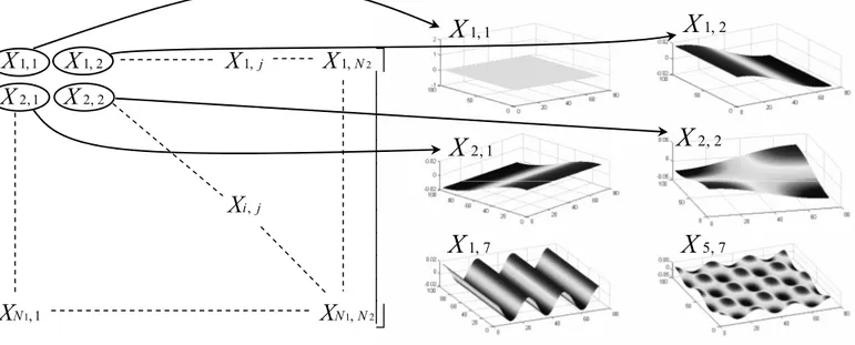
Each coefficient Xk1,k2 matches with the amplitude of a cosine function, which

frequency depends on the coefficient’s position in the matrix, from low

frequencies in the top left corner of the matrix to high frequencies in the bottom right corner.

2.2. Application to form defect

Considering the way DCT method is used in image processing, we can then imagine other domains to apply it. That was already proposed in the literature by [13]. The method was used to describe surface forms using DCT method.

Indeed, we can replace pixels and colors of images by defect’s height of a form error. We now propose to apply it with an objective of adding a technological point of view, allowing us to decompose the form error into a sum of basic technological defects. The study will be made on a plane surface. As showed earlier, position and orientation defects have already been defined by several methods. The method developed here then take into account only form defect. It could, in this perspective, be considered as a complement of 3D geometrical simulations approaches for manufacturing errors modeling, as presented in

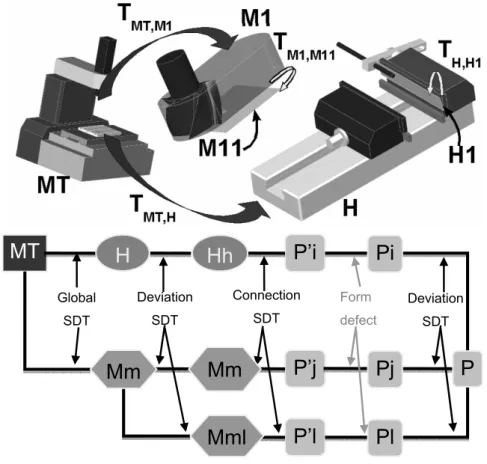
Figure 1 showing form defect integrated to the small displacements torsor

(SDT) model of manufacturing defects decomposition given in [14], with:

2 1 1 2 1,1 1, ,1 , N N N N

x

x

x

x

x

⎛

⎞

⎜

⎟

= ⎜

⎟

⎜

⎟

⎝

⎠

…

1

1

cos

((1

) 1)

cos

((1

)

)

2

2

1

1

cos

((

) 1)

cos

((

)

)

2

2

a

a

N

N

N

P

a

N

a

N

N

N

N

π

π

π

π

⎛

₊

_×

₊

_×

⎞

⎜

⎟

⎜

⎟

= ⎜

⎟

⎜

⎟

+

×

+

×

⎜

⎟

⎝

⎠

…

. .

X

=

P x P

Mm: Machining operation number m

P: Part

In this kind of model, form defect could be integrated in the global torsor chain describing manufacturing defects. In this perspective, the form error will be considered as the distance between measured points and a perfect plane associated to the real surface. To create the associated plane, we use the least square criterion, which is very efficient.

2.2.1. Surface acquiring

The first step of the method, which is the starting point to be able to apply DCT transformation, is then to measure the surface studied along a measurement grid. Indeed, the DCT method will be applied on a matrix representing measured surface, each matrix coefficient corresponding to a node on the measurement grid, its value being the measured point’s height.

The DCT coefficients matrix can then be easily found applying Eq.(3) with N1

and N2 being the measurement grid dimensions. To have an easier computation

and a better calculation time, a matrix form of equation (3) can be defined as follows in Eq.(4):

(4) with

The inverse transform is written as follows: (5)

Each term, from the DCT matrix X, matches with a cosine function, which frequency depends on its position in the matrix. Figure 2 matches a DCT matrix and the corresponding basis forms rebuilt from some of its coefficients

independently.

As the form error is calculated around the least square plane, X1,1 value will stay

to zero. Indeed X1,1 is the only matrix coefficient representing a position

displacement of the surface. Other modes then represent cosine functions, first line or column coefficients being unidirectional cosine functions (X1,2, X2,1, X1,7)

and other coefficients being bidirectional combinations of cosine functions (X2,2,

X5,7).

2.2.2. Data filtering

The DCT method then has to be applied on the set of data points representing the grid on the surface. To keep only interesting information, data has to be filtered.

Indeed, in order to study form defects only, useless information has to be rejected from the measurement signal. Positions and orientations defects have already been suppressed by considering only point’s distances from the least square plane. The next step is to remove waviness and roughness defects as well as CMM uncertainties by filtering data points obtained after the measurement operation.

It can be noticed that errors introduced by the CMM are randomly positioned around the surface on every node of the measurement grid (every millimeter). Considering the DCT matrix obtained from this grid, elementary defects

1

. .

representing errors from the CMM can be considered as a high frequency defect in the resulting DCT matrix.

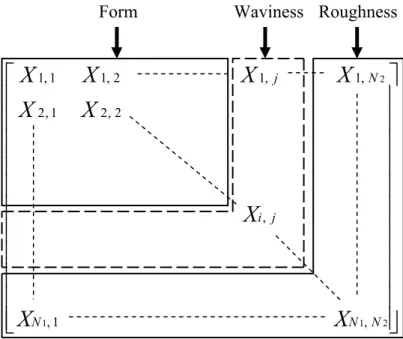
Considering the surface, form, waviness and roughness can be distinguished and sorted [15, 16]. These different defects can be classified by their wavelength. In other words, suppressing high frequencies cosine functions in the DCT matrix will allow to remove roughness defects first and waviness next, to let the signal with only the desired form defect. This distribution in the DCT matrix is

illustrated in Figure 3, highlighting the fact that form defects is described in the DCT matrix by low frequencies cosine functions, grouped in the top left of the matrix. Waviness and roughness are then described by higher frequencies cosine functions, which coefficients are placed on the right and the bottom, as

presented on the DCT matrix of Figure 3. Of course, this defects separation would have more sense on a surface theoretically measured with an endless number of points; this would lead to a surface with frequencies high enough to describe defects such as roughness. For our real case study, points have been measured every millimeter with a CMM. High frequencies coefficients in the DCT matrix won’t, practically, represent roughness defects. Actually, a CMM can’t measure roughness. For practical purposes, limits can here be changed by an experienced user function to defects he wants to observe on his surface’s form.

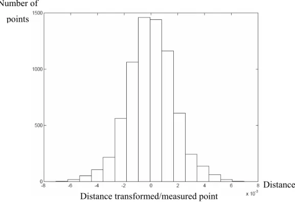
The precision of the filtered surface compared with the measured surface is function of the data filtering. Indeed, more coefficients in the DCT matrix set to zero lead to more differences between the measured and filtered surfaces. This evolution has been studied to highlight this link and try to help choosing a good compromise between data filtering and precision. A statistical comparison has been made, for different filtering levels, on measures from a real surface manufactured for method’s validation, as explained in section 3.4. For each level, the Z distance between each measured point and resulting point (after

filtering), have been calculated. Its objective is to be able to show, in a statistical point of view, if the filtered surface fits the measure surface well enough.

Table 1 presents means and standard deviations of points’ distribution. The

value studied is here the distance along Z axis between measured points and filtered surface, considering several filtering levels. A 1% filtering, for example, means that only 1% of DCT matrix coefficients are kept to their value, selecting them from the top left corner of the matrix (lower frequencies). These results help choosing the level of data filtering for the measurement grid used in our experiments. This level can change, function of the surface measured, the grid used, etc… The table and graph are here constructed from 7154 measured points (a 98x73 grid). A chart graph of points’ distribution around their mean value is shown Figure 4, for a given filtering level. It shows that filtering the surface keeps points from the filtered surface obtained normally spread around measured points.

Values calculated on Table 1 underlines preciseness of a filtered surface,

depending on the filtering level. It also underlines the fact that data filtering with DCT method does not create variations on means values.

These results then help to define an appropriate criterion for data filtering when the wavelength limit desired is not precisely known. Filtered surface accuracy can also be taken into account, comparing it, for example, with CMM

measurement uncertainties. Indeed, keeping too many coefficients, and having a filtered surface too close to the measured one will prevent us from filtering these CMM uncertainties whereas they are not desired during following steps of the method.

2.3. Results interpretation

The DCT have the advantage of being very easy to compute and being able to be applied to the form error modeling. In spite of its advantages, this method has no technological meaning. Indeed, a surface described with a sum of cosine

functions is not meaningful for a manufacturer. The objective is then to insert manufacturers’ know-how in the method. Form error studied could then be analyzed combining mathematical benefits of the DCT method with

technological meaning brought by manufacturers. In this perspective, a solution has to be found to add to the method a technological sense and, by this way, making it useful for form error technological comprehension.

This issue of having more comprehensive and meaningful results has already been encountered with other modal descriptions of form error, such as the modal tolerancing method, developed by Samper and Formosa [10]. It also describes surfaces’ form defects using a modal basis, but this one is calculated from fundamental natural modes of vibration. These modes used to describe the surface have a physical meaning, due to the way they are calculated. But, they do not often represent technical wishes or manufacturing know-how. This problem could be solved by constructing the technological basis from manufacturers’ experience.

A solution is then to create a technological basis, adapted to manufacturer’s needs, which contain every searched technological defect. These basis defects can be transformed with the DCT method, allowing mathematical operations to identify them among the global form error of a surface.

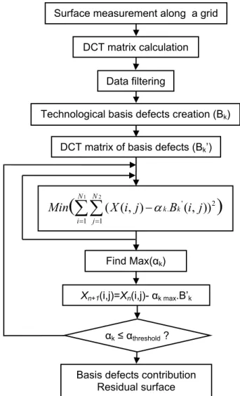
3. Technological defects identification

The next steps, on the developed method, try to find a solution to the problem of technological meaning. It consists in realizing two actions.

The first one is to create a technological defects basis that will allow us to identify technologically, and not only mathematically, the surface form error. The technological basis contains classical defects that we can encounter during manufacturing operations and is adjustable by a final user that would want to

first identify specific defects. The basis created in our further examples does not aim to be exhaustive. The objective is to show possibilities using DCT method with a technological basis and adaptability of the basis, with further objective to adapt DCT method for each process, using manufacturers’ know-how.

The next one is then to identify basis defects chosen and to tell which one are represented in the global form error. Their individual contribution to this global defect also has to be identified. The residual form is calculated and represented in order to help identifying where residual defect come from.

3.1. Technological defects basis

Once the surface has been filtered, there is only the form error left. It is then possible to start technological defects recognition. Every basis defects recorded will be identified and quantified in the final composition of the surface form.

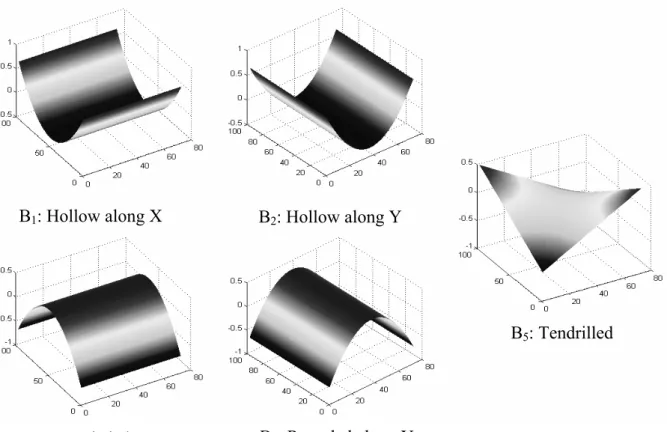
Figure 5 shows examples of basis defects that can be added to the model before

the identification phase. These basis defects can be classical defects encountered for a given process, such as geometrical defects of a machine tool, errors due to the positioning system, tool deflection,… Basis defects presented here are simulated defects added a priori.

Building a technological basis has the fundamental advantage to be speaking for itself, but it also has a mathematical inconvenience. Forms added to the basis are not always independents. Consequently, the global form error can’t be

mathematically identified as a simple linear combination of basis defects. Considering these interactions, the identification has to be made in an iterative way. Each basis defect added in the database is normed (one millimeter

3.2. Defects identification and contribution

Once the technological basis has been created, only remains the final step of the method: the identification of every basis defects and their contribution. In order to compute this identification, a criterion had to be chosen, allowing to calculate every basis defects’ significance. This criterion is developed on Equation (6), where X(i,j) and Bk’(i,j) are known, and has to be minimized to find the optimal

contribution αk of the basis defect. This equation’s optimization result leads to a

value αk that is called “basis defect contribution”, leading to a surface x(i, j),

having a minimum form defect (for only the k basis defect to be considered).

for every k basis defect (6)

Ek: criterion to minimize for every basis defect

Bk: height matrix of basis defect k (as presented in Figure 5)

Bk’: DCT matrix calculated from Bk basis defect

αk: contribution of Bk basis defect in the global form error (in mm)

Every αk contribution minimizing every Ek criterion function is calculated by the

minimization of Ek function. The defect having the biggest contribution is

identified (7) and subtracted from the global surface (8). This identification is iterated until every noticeable basis defect is identified.

for every k (7) (8)

with X0: DCT matrix of measured surface

1 2 ' 2 1 1

( ( , )

.

( , ))

E

X i j

α

B i j

=

∑∑

−

( )

Max

α

=

α

( , )

( , )

. '

X

i j

=

X i j

−

α

B

In order to have realistic results, every Ek function is minimized independently

and every αk contribution calculated separately. Indeed, the method has to be

applicable with interdependent basis defects, it is then impossible to calculate all basis defects contribution at the same time. The minimization operation ends with the calculation of a new DCT matrix Xn+1 and is then iterated on this new

DCT matrix calculated until the maximum contribution found is under a

threshold value. This value is the minimum contribution value acceptable. Each basis defect appearing in the global form error with smaller amplitude is

considered to be insignificant. In the following simulations and

experimentations αthreshold = 1µm, this value seems in this case small enough,

comparing it with measurement error of the CMM used.

Finally, the method could be described schematically as follows in Figure 6.

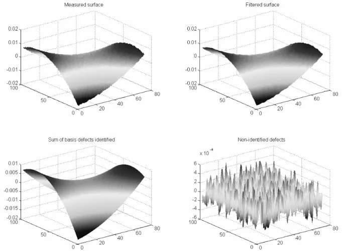
3.3. Simulation

A simulated surface has been created in order to test method’s efficiency. This surface is a combination of some basis defects presented earlier.

with B1: hollow along X, B4: rounded along Y, B5: tendrilled and

Figure 7 presents results obtained applying the method to this surface. The

simulated surface in the top left corner can be assimilated to the measured surface on a real case. A random defect with small amplitude has also been added to simulate errors introduced by CMM’s uncertainties. The filtered

surface, in the top right corner, is the result of applying a 50% filter on the DCT matrix. Bottom left corner graph presents the result of identification applied on the filtered surface. Constructed surface has here been created as a linear

combination of basis defects, the sum of basis defects identified is then very close to the constructed surface. Non-identified defects are represented in the

1 4 5

( , ) 0.025

0.012

0.004

0.0005

( , )

x i j

=

×

B

+

×

B

+

×

B

+

×

Rand i j

( , )

1

Rand i j

= ±

last graph. It is composed by defects not described in the database of classical defects.

Filtered surface is very close to constructed surface, this result seem natural. Indeed, data filtering, suppressing roughness and waviness have not an

important impact on a simulated surface, created without high frequency form defects.

Once the method has been applied, results of identified contributions can be compared with value chosen to create the simulated surface.

Basis defects identified have the following contributions:

α1=0.024946 mm α4=0.012022 mm α5=0.0040077 mm

These results are very close to the basis surfaces combination chosen to test the method. The maximum difference between simulated and identified surface is here about 5 x 10-5 mm for a αthreshold value of 1 x 10-3 mm. Furthermore,

computation is very efficient. For example, previous results have been calculated in approximately one second.

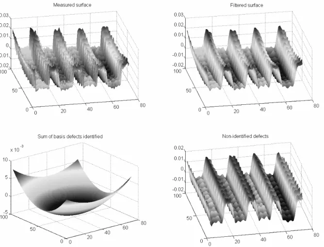
3.4. Experimentation

The method has been proven to be efficient on a simulated surface. A real case study has to be made to validate the method. The results will underline method’s advantages and limits for technological defects recognition.

To test each steps of the method, it first has been applied on plane surfaces milled with different parameters and obtained by an end milling process from an aluminum alloy rectangular part of 100x75mm. The twenty four planes have been milled with variations in the values of feed rate (from 0.1 mm/tooth to 0.2 mm/tooth), depth of cut (from 1 mm to 3 mm), tool path strategy (bi-directional and spiral end milling). Results being roughly equivalents for every tested parameter, we will only present results obtained on two of these surfaces for each tool path strategy. Indeed, as we try to decompose the global defect in a

technological database, other parameters, only changing defect’s amplitude, are not relevant.

These surfaces are measured along a grid composed by points taken every millimeter, allowing a tree dimensional reconstruction. In this case, the

measured grid’s size is 98x73 points, using a three hours measurement routine on a CMM.

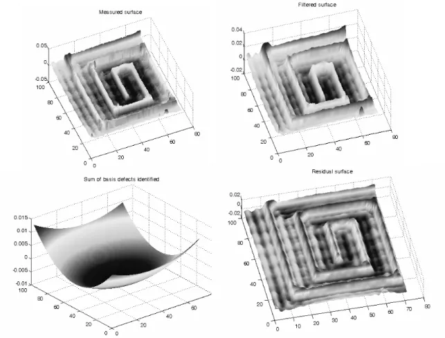
Once the surfaces have been measured, the identification can be started. In this real surface study, data filtering will have a more important role than the

previous simulated case. Residual surface is also much more important to watch here. Indeed, real surfaces are far from being composed by only basis defects. Residual defect underlines process characteristics and can highlight unexpected defects.

The method has here still been applied with a 50% filtering. Results, from

Figure 8 and Figure 9, show a filtered surface still very close to the measured

one. The basis of technological defects gives a contribution to the form error of α1=0.00686mm for B1 (hollow along X), α2=0.0034mm for B2 (hollow along Y)

and α5=0.00186mm for B5 (tendrilled plane) for the surface realized with

bidirectional strategy. The sum of these defects is represented Figure 8 and has a

2

1.1 10× − mm amplitude. Comparing it with global defects (_{3.5 10×} −2_mm

amplitude) and non-identified defect (_{2.5 10×} −2_{mm amplitude), it seems clear}

that reducing global form defect measured will come by identifying basis

defects causes, but also changing process parameters. Indeed, observing the non-identified defect allows learning about the surface. An important part of the form defect seems, in each case, to follow the tool path. It can be considered as a consequence of tool deflection due to cutting forces. This “tool path signature” can be added to the identification database for an improved defect’s

3.5. Technological basis improvement

The technological basis, first constructed without a real knowledge of the process and the form defect induced, can be insufficient for a complete

identification. It can then be adapted after a further look into the residual defect obtained with the previous technological basis used.

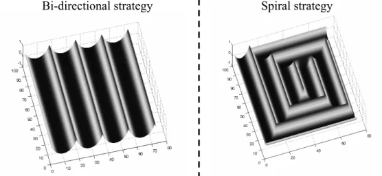
For the case studied in section 3.4, the residual defect mainly seemed to come from tool deflection along the tool path chosen. As we tried to develop an adaptive method, it is possible to complete the technological basis used from previous observations. A new technological defect is added to the basis, called “tool deflection”. It is constructed automatically from geometrical information (trajectory coordinates and tool size) and integrated for the identification step of the method. Basis defects created can be seen on Figure 10, one built from coordinates of the bi-directional strategy and the other one from coordinates of the spiral strategy.

A new decomposition is made using adapted technological basis. Results are presented on Table 2, comparing identified contributions obtained before and after using tool deflection defect, B1 corresponding to first technological basis used and B2 to completed technological basis. Figure 11 present visual results of the identification for the bi-directional strategy and the spiral strategy, with basis defects identified on the top and residual defects on the bottom. These results are to compare with Figure 8 and Figure 9 results. In order to compare them, a variance criterion is calculated in each case, comparing the variance of distances between residual surface and the least square plane. Identified defects now give a good image of the real surface. The technological basis used seems adapted to the process used here (end milling).

4. Conclusion

The discrete cosine transform method has been studied, in particular its

mathematical properties, trying to notice the method’s advantages with a view to apply it for our purpose: modeling form error of manufactured surfaces with a technological point of view. As well as fitting very well the measured surface, DCT method gives a surface description as a sum of cosine functions sorted, in the DCT matrix obtained, by frequencies. This property helps surface filtering and allows dividing surface information (form, waviness, roughness). This way to describe and filter surface form, particularly when using its matrix form, is also easy to compute and very efficient considering calculation time.

In addition to method’s mathematical advantages for surface form description, we showed in this paper that a technological significance can be added to the method. Results, obtained modeling surface form error, are then meaningful for manufacturers. The possibility to create an identification database, adaptable to classical form defects encountered for a given process, leads to this meaningful description as a sum of technological defects. Error causes can then be studied separately, considering their contribution to the global error measured.

Two ways can then be explored to apply the method. First, the technological form defects identification; in this case the method can be applied alone,

considering form defects from the least square surface on the manufactured part. This way to apply the method aims to help manufacturers to quantify classical basis defects and underline systematic defects created by a given production mean. Then, process plan simulation for tolerance specifications respect; the method has, in this case, to be applied as a complement to existing methods for three dimensional process plan simulation. The method then adds the form

defect characterization to calculated position and orientation defects and leads to a complete definition of manufactured parts surfaces.

References:

[1] L. Mathieu, A. Ballu, “A Model for a Coherent and Complete Tolerancing Process”, 9th CIRP Seminar on Computer Aided Tolerancing, Arizona, p.35-44, 2005.

[2] B. Anselmetti, “Generation of functional tolerancing based on positioning features”, Computer Aided Design, n°38, p. 909-919, 2006.

[3] M. Giordano, B. Kataya, E. Pairel, “Tolerance analysis and synthesis by means of clearance and deviation spaces”, selected article 7th CIRP, Kluwer, Academic Publishers, p.145-154, 2003.

[4] S.H. Ryu, C.N. Chu, “The form error reduction in side wall machining using successive down and up milling”, Int. J. Mach. Tools Manuf., n°45, p.1523-1530, 2005.

[5] W.-S. Yun, J.H. Ko, D.-W. Cho, K.F. Ehmann, “Development of a virtual machining system, part 2: prediction and analysis of a machined surface error”, Int. J. Mach. Tools Manuf., n°42, p.1607-1615, 2002.

[6] P. Dépincé, J.-Y. Hascoët, “Active integration of tool deflection effects in end milling. Part 1: Prediction of milled surfaces”, Int. J. Mach. Tools Manuf., n°46, p.937-944, 2006.

[7] S. Tichadou, O. Legoff, J.-Y. Hascoët, “3D Geometrical simulation of manufacturing. Compared approaches between integrated CAD/CAM system and small displacement torsor model”, Advances in integrated Design and

Manufacturing in Mechanical Engineering, p. 446-456, Kluwer, Dordecht, 2005. [8] F. Vignat, F. Villeneuve, “Simulation of the manufacturing process (2): Analysis of its consequence on a functional tolerance”, Proceedings of the 9th CIRP Computer Aided Tolerancing Seminar, Tempe, Arizona, 2005.

[9] E. Dimas, D. Briassoulis, “3D geometric modeling based on NURBS: a review”, Advances in Engineering Software, n°30, p.741-751, 1999.

[10] S. Samper, F. Formosa, “Defects Tolerancing by Natural Modes Analysis”, Journal of Computing and Information Science in Engineering Volume 7, Issue 1, p. 44-51, 2007.

[11] N. Ahmed, T. Natarajan, K.R. Rao, “Discrete Cosine Transform”, IEEE Transactions on Computers, p.90-93, 1974.

[12] B. Josso, D. R. Burton, M. J. Lalor, “Frequency normalised wavelet transform for surface roughness analysis and characterisation”, Wear, n°252, p.491-500, 2002.

[13] W. Huang, D. Ceglarek, “Mode-based Decomposition of Part Form Error by Discrete-Cosine-Transform with Implementation to Assembly and Stamping System with Compliant Parts”, CIRP Annals – Manufacturing Technology, Volume 51, Issue 1, p.21-26, 2002.

[14] O. Legoff, S. Tichadou, J.-Y. Hascoët, “Manufacturing errors modeling: two three dimensional approaches”, International Journal of Engineering and Manufacturing, Vol. 218 – Part B, p.1869-1873, 2004.

[15] J. Raja, B. Muralikrishnan, S. Fu, “Recent advances in separation of

roughness, waviness and form”, Precision Engineering, n°26, p. 222-235, 2002. [16] S. Mezghani, H. Zahouani, “Characterization of the 3D waviness and roughness motifs”, Wear, n°257, p.1250-1256, 2004.

Figure 1: Torsor chain in 3D geometrical simulation in manufacturing MT P’i P’l P’j Global SDT Deviation SDT Connection SDT Pi Pl Pj Form defect Mm Mm Mml P H Hh Deviation SDT

Figure 2: DCT matrix coefficients 2 1 1 2 1, 1 1, 2 1, 1, 2, 1 2, 2 , , 1 , j N i j N N N X X X X X X X X X ⎡ ⎤ ⎢ ⎥ ⎢ ⎥ ⎢ ⎥ ⎢ ⎥ ⎢ ⎥ ⎢ ⎥ ⎢ ⎥ ⎢ ⎥ ⎢ ⎥ ⎢ ⎥ ⎢ ⎥ ⎣ ⎦ 1, 1

X

X

X

X

X

X

Figure 3: Defects distribution in DCT matrix 2 1 1 2 1, 1 1, 2 1, 1, 2, 1 2, 2 , , 1 , j N i j N N N

X

X

X

X

X

X

X

X

X

⎡

⎤

⎢

⎥

⎢

⎥

⎢

⎥

⎢

⎥

⎢

⎥

⎢

⎥

⎢

⎥

⎢

⎥

⎢

⎥

⎢

⎥

⎢

⎥

⎣

⎦

Figure 4: Points distribution for a 50% filtering

Distance transformed/measured point Number of

points

Figure 5: Basis defects samples

B3: Rounded along X B4: Rounded along Y

B2: Hollow along Y

B1: Hollow along X

Figure 6: Technological defects recognition

Surface measurement along a grid

DCT matrix of basis defects (Bk’)

DCT matrix calculation Data filtering

Technological basis defects creation (Bk)

1 2 ' 2 . 1 1 ( ( , ) ( , ))

(

)

∑∑

Xn+1(i,j)=Xn(i,j)- αk max.B’k

αk ≤ αthreshold ?

Basis defects contribution Residual surface

Figure 10: Tool deflection defect

Figure 11: Results with improved basis

Table 1: Precision function of filtering

Type of filtering   1%  4% 9%  16% 25% 36%  49%  64% 81%

Mean value  ≈ 0 

Table 2: Compared identification results

Identification results

Bi-directional strategy Spiral strategy

B1 B2 B1 B2 Hollow along X (mm) 0 0 0 0 Hollow along Y (mm) 0 0 0 0 Rounded along X (mm) 0.0102 0.0102 0.0125 0.0136 Rounded along Y (mm) 0.0039 0.002 0.0046 0.0043 Tendrilled (mm) 0.0014 0.0014 0.0029 0.0028 Tool deflection (mm) 0.0199 0.0222 Variance (x10-5 mm) 4.56 1.33 3.31 1.02