HAL Id: hal-00329311
https://hal.archives-ouvertes.fr/hal-00329311
Submitted on 8 Apr 2004
HAL is a multi-disciplinary open access
archive for the deposit and dissemination of
sci-entific research documents, whether they are
pub-lished or not. The documents may come from
teaching and research institutions in France or
abroad, or from public or private research centers.
L’archive ouverte pluridisciplinaire HAL, est
destinée au dépôt et à la diffusion de documents
scientifiques de niveau recherche, publiés ou non,
émanant des établissements d’enseignement et de
recherche français ou étrangers, des laboratoires
publics ou privés.
boundary structure and magnetic field depletions
P. J. Cargill, M. W. Dunlop, B. Lavraud, R. C. Elphic, D. L. Holland, K.
Nykyri, A. Balogh, I. Dandouras, H. Rème
To cite this version:
P. J. Cargill, M. W. Dunlop, B. Lavraud, R. C. Elphic, D. L. Holland, et al.. CLUSTER encounters
with the high altitude cusp: boundary structure and magnetic field depletions. Annales Geophysicae,
European Geosciences Union, 2004, 22 (5), pp.1739-1754. �hal-00329311�
CLUSTER encounters with the high altitude cusp: boundary
structure and magnetic field depletions
P. J. Cargill1, M. W. Dunlop1,2, B. Lavraud3, R. C. Elphic4, D. L. Holland5, K. Nykyri1, A. Balogh1, I. Dandouras3, and H. R`eme3
1Space and Atmospheric Physics, Blackett Laboratory, Imperial College, London SW7 2BW, UK 2Space Science Department, Rutherford Appleton Lab., UK
3Centre d’Etude Spatiale des Rayonnements, Toulouse, France 4Los Alamos National Laboratory, Los Alamos, USA
5Dept. of Physics, Illinois State University, Normal, IL, USA
Received: 11 July 2003 – Revised: 20 January 2004 – Accepted: 23 January 2004 – Published: 8 April 2004
Abstract. Data from the four spacecraft Cluster mission
during a high altitude cusp crossing on 13 February 2001 are presented. The spacecraft configuration has one lead-ing spacecraft, with the three traillead-ing spacecraft lylead-ing in a plane that corresponds roughly to the nominal magnetopause surface. The typical spacecraft separation is approximately 600 km. The encounter occurs under conditions of strong and steady southward Interplanetary Magnetic Field (IMF). The cusp is identified as a seven-minute long depression in the magnetic field, associated with ion heating and a high abundance of He+. Cusp entry involves passage through a
magnetopause boundary that has undergone very significant distortion from its nominal shape, is moving rapidly, and ex-hibits structure on scales of the order of the spacecraft sepa-ration or less. This boundary is associated with a rotation of the magnetic field, a normal field component, and a plasma flow into the cusp of approximately 35 km/s. However, it cannot be identified positively as a rotational discontinuity. Exit from the cusp into the lobe is through a boundary that is initially sharp, but then retreats tailward at a few km/s. As the leading spacecraft passes through this boundary, there is a plasma flow out of the cusp of approximately 30 km/s, sug-gesting that this is not a tangential discontinuity. A few min-utes after exit from the cusp, the three trailing the spacecraft see a single cusp-like signature in the magnetic field. There is an associated temperature increase at two of the three trailing spacecraft. Timing measurements indicate that this is due to cusp-like regions detaching from the rear of the cusp bound-ary, and moving tailward. The magnetic field in the cusp is highly disordered, with no obvious relation between the four spacecraft, indicative of structure on scales <<600 km. However, the plasma moments show only a gradual change over many minutes. A similar cusp crossing on 20 Febru-Correspondence to: P. J. Cargill
ary 2001 also shows a field depression and highly dynamic boundaries.
Key words. Magnetospheric physics (magnetopause, cusp
and boundary layers; solar wind-magnetosphere interac-tions) – Space plasma physics (discontinuities)
1 Introduction
The high-altitude cusps are important regions of the magne-tosphere, and play a key role in the transport of solar wind energy to both the nightside magnetosphere and the auroral regions. In an idealised situation, they are the location where the magnetosheath flow encounters a location along the mag-netopause, where the sign of the terrestrial field reverses with respect to the flow direction. Their complexity stems from (a) the comparable levels of the energy density in the magnetic field, plasma bulk flow and “thermal” plasma and (b) the re-mote influence exerted on the cusp by magnetic reconnection at various magnetopause locations. The high-altitude cusps were explored in the 1970s by the Hawkeye and HEOS–1 and –2 spacecraft (e.g. Paschmann et al., 1976; Farrell and Van Allen, 1990; Kessel et al., 1996; Eastman et al., 2000; Dun-lop et al., 2000), and significant recent advances have also come from the POLAR and Interball spacecraft (e.g. Zhou and Russell, 1997; Merka et al., 2000; Sandahl et al., 2000; Stubbs et al., 2001; Scudder et al., 2002). POLAR, in partic-ular, has presented a picture of an extended cusp (dimensions many RE: Grande et al., 1997; Fritz et al., 2003), populated
by particles of solar wind and ionospheric origin (e.g. Grande et al., 1997; Chen and Fritz, 1998; Chang et al., 2000). In ad-dition, both Hawkeye and POLAR have provided evidence for the elusive so-called “lobe reconnection” (Dungey, 1963; Kessel et al., 1996; Scudder et al., 2002).
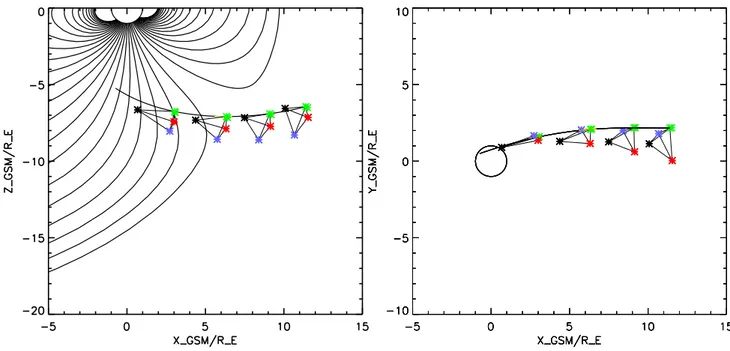
Fig. 1. The Cluster orbit between 16:00 and 23:59 UT on 13 February 2001 in the x-z GSM plane (left panel) and x-y GSM plane (right
panel). The spacecraft are colour-coded (black, red, green and blue for spacecraft 1–4, respectively). The spacecraft are first shown at 16:00 and then at two hour intervals. T89 model field lines are shown in Fig. 1a. The spacecraft separations shown are 20 times larger than in reality, with spacecraft 3 being shown at its real location.
The four-spacecraft Cluster mission was launched in July and August 2000, with the principal aim of carrying out multi-spacecraft, multi-instrument studies of the Earth’s space plasma environment. One of the major scientific goals was to carry out observations of the high altitude, high lati-tude cusp regions. Cluster has the ability to determine abso-lute motions, scales and electric currents by the use of multi-ple spacecraft. In addition, with its apogee of 20 RECluster
is expected to fly through the cusp/magnetopause boundary on its way to and from the solar wind, thus sampling differ-ent regions of the cusp from POLAR, whose apogee is 8.9
RE. The orbit also suggests that the encounters Cluster has
with the cusp may be shorter lived than those experienced by POLAR. In its first year of operation, Cluster had en-counters with the central cusp in the February/March time interval at high altitudes and in August/September for lower altitudes (4–5 RE: Cargill et al., 2001). Due to the nature
of the orbit, the inbound (southern) and outbound (northern) crossings sample different regions of the high altitude cusp (e.g. Lavraud et al., 2004; Dunlop et al., 2004). We also note that, due to limited facilities for returning data from the spacecraft, there are fewer inbound than outbound crossings in 2001 and 2002, a situation remedied from early 2003.
The outbound crossings have been documented by Lavraud et al. (2002, 2004) and Vontrat-Reberac et al. (2003). Lavraud et al. discussed one case on 4 Febru-ary 2001, where the cusp was composed of largely stagnant plasma with low magnetic field strength (referred to as the stagnant exterior cusp). Cluster spent more than 1 h in this re-gion, and exited through an as-yet-unidentified boundary into
the magnetosheath. Vontrat-Reberac et al. (2003) discussed a crossing on 17 March 2001, where Cluster remained in the cusp for 1.5 h, but in a region dominated by the magnetic field. In this case the IMF was weakly north, yet the cusp was filled with magnetosheath plasma and copious magnetic field turbulence. Exit from the cusp on this occasion was through the dayside magnetosphere.
Cargill et al. (2001) identified an inbound crossing on the basis of a 7–8 min drop-out in the magnetic field strength around 20:00 UT on 13 February 2001 during a period of strong southward IMF. This paper presents a more complete study of the magnetic field and plasma properties for this en-counter. A superficially similar inbound event was seen a week later at 23:20 on 20 February 2001 (Elphic et al., 2001), but in this case the IMF was initially northward, with a south-ward turning near the time of cusp entry. This second case was obtained during a conjunction between the FAST space-craft and Cluster (Elphic et al., 2001). The relationship of these crossings to the outbound ones mentioned above is not completely clear at this time, but probably reflects the fact that the inbound passes sample a more limited part of the cusp.
In Sect. 2, we review briefly the relevant instrumentation, and discuss the spacecraft formation for both cases. Sec-tions 3 and 4 examine the 13 February 2001 crossing in de-tail. Section 3 looks at the encounter from the viewpoint of single spacecraft phenomenology, and Sect. 4 addresses multi-spacecraft results, such as motions and scales. Sec-tion 5 presents a brief summary of the 20 February crossing.
3.98 4 4.02 4.04 4.06 x 10⁴ −9200 −9100 −9000 −8900 −8800 −8700 −8600 X GSE(km) Y GSE (km) 3.98 4 4.02 4.04 4.06 x 10⁴ −4.68 −4.67 −4.66 −4.65 −4.64 −4.63 −4.62 X GSE(km) Z GSE (km) −9200 −9000 −8800 −8600 −4.67 −4.66 −4.65 −4.64 −4.63 x 10⁴ Y GSE(km) Z GSE (km) 4 4.02 4.04 4.06 x 10⁴ −9000 −8800 −4.67 −4.66 −4.65 −4.64 −4.63 x 10⁴ X GSE(km) Y GSE(km) Z GSE (km)
Fig. 2. The spacecraft configuration at 20:00 UT on 13 February 2001. The four panels show the tetrahedron projected onto the GSE x–y, x–z
and y–z planes, and a three-dimensional representation of the spacecraft formation. The four Cluster spacecraft are denoted by the coloured dots. The blue arrows correspond to the direction of the spacecraft motion projected onto the appropriate plane. Their length is proportional to the velocity projected onto each plane.
2 Instrumentation and spacecraft formation
Each Cluster spacecraft has a complement of 11 instruments covering a wide range of electromagnetic field and plasma measurements. In this paper, we use data from the Cluster flux gate magnetometers (FGM: Balogh et al., 1997; 2001) and the Cluster Ion Spectrometer (CIS: R`eme et al., 2001). Unless otherwise stated, we show spin-averaged magnetic field data (i.e. one vector every 4.1 s), but also use higher resolution data (22 vectors/s) as required. To analyse the ion properties, we present data from both the Hot Ion Analyser (HIA) and the ion COmposition and DIstribution Function analyser (CODIF). The former is used to provide moments of the measured ion distribution function, while the latter provides moments and spectrograms of H+, He++, He+and O+. The basic HIA moments are available every 4.1 s, and we focus on the density, velocity vector and temperatures.
Parallel (T||), perpendicular (T⊥)and total (T) temperatures
are available, where T=(2 T⊥+T||)/3. The CODIF
spectro-grams use data with a resolution of 4 spins (i.e. just over 16 s).
The spacecraft orbit and configuration is best understood in the context of the 13 February encounter (that on 20 Febru-ary was similar in almost all respects, being just 7 days later). We concentrate on the time interval from 19:30–21:00 on 13 February, since this corresponds to the cusp crossing. Figures 1a and b show the Cluster orbit during the interval 16:00–23:59, with 1a and 1b showing projections onto the X–Y and X–Z GSM planes, respectively (in the latter case, Cluster is coming out of the paper). In Fig. 1a field lines com-puted according to the Tsyganenko (1989) model are shown. The spacecraft are colour-coded (black, red, green and blue for spacecraft 1–4, respectively). In these plots, the space-craft separation vectors are a factor 20 larger than in reality.
0 5 10 |B|(nT) −50 5 10 B x −10 0 10 B y −15 −10−5 0 5 B z 0 5 10 n(cm −3 ) 400 500 600 v(km/s) 19:000 19:15 19:30 19:45 20:00 20:15 20:30 20:45 21:00 2 4 P D (nPa)
13 February (UT): GSE lagged
Fig. 3. Lagged solar wind data from the ACE spacecraft for the interval 19:00–21:00 UT on 13 February 2001. The six panels show |B|, Bx,
Byand Bz(in GSE coordinates), n, V and the dynamic pressure. A constant lag velocity of 530 km/s and lag time of 42 min was used.
For example, 2 RE on the plots corresponds to a physical
separation of approximately 600 km. The four configurations are at 16:00, 18:00, 20:00 and 22:00, respectively, with later times being inside the magnetopause. The spacecraft config-urations are shown at the time along the orbit, corresponding to the location of spacecraft 3 (green).
The four Cluster spacecraft form a tetrahedron. The four panels of Fig. 2 show the spacecraft formation projected on the GSE x–y, x–z and y–z planes, and a three-dimensional representation of the formation. The dark blue arrows show the direction of motion of each spacecraft, and the yellow shaded surface is that bounded by lines joining spacecraft 1, 3 and 4. Around 20:00 UT (the most interesting time), the formation had spacecraft 1 leading, with spacecraft 2–4 trailing, and forming a plane that is approximately parallel to the nominal plane of the magnetopause (based on the Tsy-ganenko, 1989 model). The formation is displaced approx-imately 1.5 RE in the GSE–y direction from the Sun-Earth
line (Fig. 2a: in GSM coordinates, Cluster is displaced ap-proximately 2 REin the positive y direction). One might
ex-pect any magnetopause or cusp crossing to be seen first by spacecraft 1, and then by the other three in quick succession. The separations on 20 February are very similar. The ve-locity of the formation is given by the vector (−2.7, −0.62, 0.22) km/s in GSE coordinates.
3 Overall description of cusp encounter of 13 February
3.1 Solar wind conditions
Figure 3 shows the solar wind conditions between 19:00 and 21:00 UT obtained from the ACE spacecraft, located in the vicinity of the L1 point 235 RE upstream of the Earth. The
solar wind was quite steady over the time of interest, and the velocity of 500 km/s implies a fairly constant “lag time” of between 42 and 48 min for solar wind features to reach the cusp (in view of the uncertainties of propagation mod-els from L1 to the cusp, we do not believe a more rigor-ous analysis of the lag time is warranted here). Figure 3 assumes a velocity of 530 km/s and a lag time of 42 min.
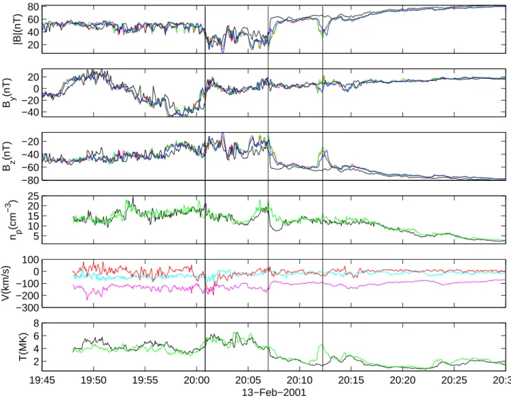
20 40 60 |B|(nT) −40 −20 0 20 B y (nT) −80 −60 −40 −20 B z (nT) 5 10 15 20 25 n p (cm −3 ) −300 −200 −100 0 100 V(km/s) 19:45 19:50 19:55 20:00 20:05 20:10 20:15 20:20 20:25 20:30 2 4 6 8 T(MK) 13−Feb−2001
Fig. 4. An overview of the magnetic field and plasma parameters between 19:45 and 20:30 UT on 13 February 2001. The six panels show |B|, ByBz, n, V and T. The x, y and z components of the plasma velocity seen by spacecraft 3 are denoted by cyan, red and magenta lines in
panel 5. The three vertical lines refer to features discussed in the text. There is a data gap in the plasma data before 19:48.
The density was also roughly constant at 5 cm−3. For the 2 h shown, the interplanetary magnetic field (IMF) strength declined very smoothly from 10 to 7 nT. However, from the viewpoint of the cusp, the important aspect is the behaviour of the y and z IMF components within this smoothly varying field magnitude. The dominant component of the IMF was southward, with a magnitude between 9 and 6 nT. There was a brief weakening of the southward IMF lasting 1–2 min at around 19:48. The y component of the IMF was weaker (be-low 5 nT). Such an IMF topology, mainly southward in the whole interval, might be expected to drive strong magnetic reconnection in the vicinity of the sub-solar point (Dungey, 1961), although we note that under the anti-parallel merging hypothesis (Crooker, 1979), the intermittent y-components of the IMF would lead to merging elsewhere (e.g. Maynard et al., 2001). In either case the net result is likely to be a disturbed magnetosphere. The geomagnetic conditions for 20:00 on 13 February were a Dst index of −40 nT, and a Kp
value of 4.
3.2 Cusp phenomenology
We now discuss the overall phenomenology of the cusp, as seen from a single spacecraft point of view. Multi-spacecraft aspects are presented in the next section. Figure 4 shows an overview of the cusp encounter between 19:45 and 20:30. The six panels show spin-averaged magnetic field data [|B|, By, Bz] from FGM on all spacecraft (panels 1–3), the
den-sity and temperature from the CIS instruments on spacecraft 1 and 3 (panels 4 and 6), and the three components of the plasma velocity seen by spacecraft 3 are denoted by cyan (Vx), red (Vy)and magenta (Vz)lines in panel 5. GSE
co-ordinates are used. The cusp is identified as the clear depres-sion in the total field strength commencing at around 20:00, and lasting until approximately 20:07, with a cusp re-entry seen by the trailing three spacecraft at 20:12. (In the termi-nology of Lavraud et al. (2002), this would be the exterior cusp, but here it is just referred to as the cusp.) The magnetic boundaries are clear and distinct, are indicated by the vertical lines, and could be interpreted as a magnetopause crossing at
Fig. 5. Data from the CODIF instrument on spacecraft 1 between 19:45 and 21:00 on 13 February 2001. The three colour panels show
the energy spectrograms for H+, He++and He+, respectively, between 10 and 40 000 eV. The flux colour palate is shown at the right. For context, the lower panel shows the magnetic field magnitude.
20:00, exit through the cusp rear into the lobe at 20:07, with a cusp re-entry and exit at 20:12. We identify 20:00 as the magnetopause, since that is where the y-component of the field becomes “terrestrial-like”: a classic magnetopause def-inition. For a spacecraft velocity in the x-direction of 2.7 km/s, this leads to a cusp width of approximately 1200 km. The narrow width of the cusp compared to other cases ob-served by Cluster (104km: e.g. Lavraud et al., 2002, 2004; Vontrat-Reberac et al., 2003) suggests that we are passing through the very tailward part of a longer (along the magne-topause) cusp structure.
In the magnetosheath between 19:00 and 20:00, the field lies predominately in the southward direction, as expected from the draping of a southward IMF around the magne-topause. Prior to entry into the cusp, there is an excursion in Byup to 30 nT and then down to −40 nT that lasts 13 min,
while the total field strength remains constant. We are un-able to associate the By feature with anything seen in the
solar wind by ACE, but note that in the three hours prior to cusp entry, there are other equally clear By features in the
magnetosheath (not shown).
The HIA ion measurements show a more diffuse, extended structure than seen in the magnetic field. From the viewpoint of the density, the FGM cusp entry at 20:00 is visible as a
very slight decrease, the exit as a pulse followed by a sharp decrease, whereas the 20:12 re-entry is not evident at all. The density then gradually tails off up to 20:30 UT. The velocity shows the expected dominant southward flow of the magne-tosheath plasma as it moves around the magnetopause, but this flow persists in both the cusp and magnetosphere, in-dicating that field lines are being swept tailward, presum-ably due to continual magnetic reconnection at the sunward magnetopause. There is also a deflection of the velocity in the negative y-direction on cusp entry, lasting approximately 1–2 min. For a southward IMF, a strong, positive (negative) By orientation will lead to plasma flows in the duskwards
(dawnwards) directions, so the negative Vyis consistent with the negative By on cusp entry. We note here that this cusp
encounter with its strong directional flow is very different from the “stagnant cusp” discussed elsewhere in the literature (e.g. Lavraud et al., 2002, 2004). The temperature moments (lower panel) show ion heating in the cusp by a factor of about 50% (especially perpendicular to the field: not explic-itly shown). There is additional plasma heating at the field re-entry at 20:12 (spacecraft 3) and 20:14 (spacecraft 1), and perhaps at 20:23–20:28, but with no obvious field signature at the last of these times.
20 40 |B| −10 0 10 B x −40 −20 0 20 B y −50 0 B z −50 0 θ 19:58 19:59 20:00 20:01 20:02 20:03 20:04 20:05 20:06 20:07 20:08 20:09 20:10 100 200 300 φ UT (Feb 13, 2001)
Fig. 6. The magnetic field with a resolution of 22.4 vectors per second from 19:58–20:10 UT on 13 February 2001. The six panels show the
magnetic field magnitude, components and orientations (expressed as the angles θ and φ) in GSE coordinates.
Figure 5 shows measurements from the CODIF instrument (R`eme et al., 2001) on spacecraft 1 for the interval 19:30– 21:00. The first three panels show energy spectrograms for H+, He++ and He+. It is instructive to compare the abun-dances of H+ (also He++) and He+, since these can be viewed as being “tracers” for solar wind and ionospheric (or plasmaspheric) particles, respectively. (Note that the CODIF sensor is slightly saturated in the magnetosheath. In addition, some spillover from the H+population is occurring, and re-sults in nonnegligible background count rates in the He++ and He+spectrogram throughout the passage (this is, for in-stance, obvious in the magnetosheath, where He+should be nearly absent). However, it is clearly seen that the H+ and He++ fluxes are varying coherently, confirming their com-mon solar wind origin.)
On entry to the exterior cusp at 20:00, there is an im-mediate (within 1 bin) large increase in the He+count rate, with particles of energy between 1 and 10 keV being de-tected. Bearing in mind the instrumental caveat noted above,
the comparison of the various fluxes in the spectrograms of Fig. 5, as well as the detailed examination of time-of-flight spectra from the CODIF instrument (not shown), unambigu-ously demonstrates that the He+flux increase reflects the ef-fective presence of a large amount of singly charged Helium ions of ionospheric (or plasmaspheric) origin in the exterior cusp. It should be noted that the presence of high energy He+ fluxes in the magnetosheath adjacent to the boundary indicates a probable leakage.
The He+enhancement persists throughout the low
mag-netic field exterior cusp. The flux appears lower near the exterior cusp-plasma mantle boundary, but large fluxes are again measured shortly afterward, albeit at lower energies (500 eV–1 keV). This He+component terminates roughly at 20:27. The presence of such He+ abundances is not com-mon in the exterior cusp region, and the large change in mean energy observed when compared to those measured in the plasma mantle is intriguing. The only plausible source of such amounts of He+ is from the ionosphere. We must
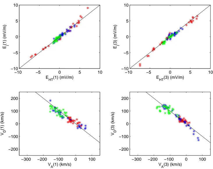
−300 −200 −100 0 100 −200 −100 0 100 200 VA(1) (km/s) V D (1) (km/s) −300 −200 −100 0 100 −200 −100 0 100 200 VA(3) (km/s) V D (3) (km/s) −10 −5 0 5 10 −10 −5 0 5 10 EHT(1) (mV/m) E j (1) (mV/m) −10 −5 0 5 10 −10 −5 0 5 10 EHT(3) (mV/m) E j (3) (mV/m)
Fig. 7. The upper panels show the relation between Ejand EH T for the interval 19:59:30–20:01:30 for spacecraft 1 (left) and 3 (right). The
correlation coefficients are 0.983 and 0.987, respectively, indicating the existence of a deHoffman-Teller frame. The lower panels show the relation between vj−VH T and VAfor the same time interval. A linear relationship would indicate that the Walen relations were satisfied,
and that the boundary was a rotational discontinuity. In all plots, red, blue and green points correspond to the x, y and z components of the relevant vectors. The black lines correspond to a slope of unity.
assume that the strong electric fields induced in the inner magnetosphere and ionosphere during times of strong and persistent southward IMF are injecting large amounts of He+
onto the cusp field lines.
4 Cusp structure from a multi-spacecraft perspective
From the single spacecraft perspective, the cusp is magneti-cally a structure with clear boundaries demarking regions of field depletion. We now analyse the boundaries of these re-gions using higher resolution magnetic field data.
4.1 Cusp entrance
High-resolution (22.4 vectors per second) FGM data from the interval 19:59–20:10 are shown in Fig. 6. The panels show |B|, Bx, By, Bz, θ=sin−1(Bz/|B|) and
φ=cos−1(Bx/|B2x+B2y|). Consider first the field magnitude
(top panel). We show the start and finish of cusp entry (as de-fined by the decrease in field magnitude) by the first two solid lines. Cusp entry is through a boundary of duration just over a minute, occurs to within a few seconds at all spacecraft, and sees the y- and x-components of the magnetosheath field largely switched off.
We have performed a minimum variance analysis (MVA: Sonnerup and Scheible, 1998) using the spin-averaged data (to reduce small-scale fluctuations) over the interval 19:59:30–20:01:30. These times mark the transition to and from relatively homogeneous magnetic fields, but a shorter interval (20:00–20:01) shows no significant differ-ence. “Good” normals (minimum to intermediate eigenvalue ratios of the order of 10 or greater) are found for spacecraft 1, 3 and 4 (λ2/ λ3=9.2, 14.3 and 13.7, respectively), but not
B2and B3for spacecraft 2 show similar behaviour to those
on spacecraft 1, 3 and 4. Despite the low eigenvalue ratio, we believe that spacecraft 2 is seeing a similar boundary to the others. The average normal from spacecraft 1, 3 and 4 is given by n=(0.96, −0.21, −0.16), with an average nor-mal field of 3.6 nT, consistent with a field directed outward through the boundary. There is a flow normal at the bound-ary of −35 km/s (i.e. inward to the cusp), which should be contrasted with an Alfv´en speed of 170 km/s. The bound-ary is thus oriented in a direction such that its normal points largely sunward, but also dawnward. This should be con-trasted with the normal of a model magnetopause, nMP=(0.6,
0.15, −0.75). Thus, the magnetopause here has undergone considerable distortion. The discontinuity analyser (Dunlop et al., 2002) can also be applied to this boundary and gives an average outward motion of 30 km/s (Dunlop et al., 2004). We have also carried out the standard test for a deHoffman-Teller (dHT) frame for this interval for space-craft 1 and 3. We find VH T= −(68, 128, 242) km/s and
−(72, 104, 255) km/s for spacecraft 1 and 3, respectively. The results change by perhaps 10% when different intervals are considered. The quality of the dHT frame can be assessed by examining the correlation between the two electric fields
Ej=−vjxBj and EH T=−VH TxBj. The correlation
coeffi-cient is 0.983 and 0.987 for spacecraft 1 and 3, as shown in the top panels of Fig. 7. The lower panels show the result of testing the Walen relations (vj−VH T versus VA)for
space-craft 1 and 3 (Khrabrov and Sonnerup, 1998). For all panels, the black slope has a slope of unity and is included for guid-ance. We find that there is no precise linear relation between the two vectors, but for the three components at spacecraft 1 (3) there are negative slopes of 0.54, 0.82 and 0.6 (0.52, 1.12 and 0.36) for each vector. Consideration of all components gives negative slopes of approximately 0.8. Any identifica-tion as a rotaidentifica-tional discontinuity (RD) is thus non-definitive, and variations of the interval length under consideration do not lead to any clarification.
The properties of the boundary can be summarised as fol-lows. There is a normal plasma flow, no clear density jump, a decrease in the field magnitude, a rise in the temperature, a plasma flow in the y-direction and a rotation of the field from having three components to pointing predominately in the z-direction. A variety of MHD boundaries satisfy some of these conditions, but none satisfy them all. For example, a RD is the only boundary that can sustain a non-coplanar field rotation, but should not have some of the other features seen, such as magnetic field and temperature changes. A slow shock can give a temperature increase, field decrease and y-flow, but is not consistent with the observed field rota-tion. However, it is clear that the boundary is not a tangential discontinuity, since there is a normal plasma flow. It should be noted that many of these properties were also noted at the cusp-magnetosheath boundary by Lavraud et al. (2002).
Another possibility is that two of these discontinuities ex-ist in close proximity to each other: for example, a RD first rotates the field, and then a slow shock decreases the field
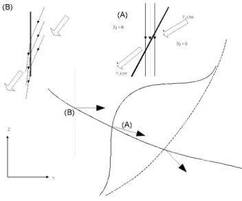
Fig. 8. A sketch of the cusp encounter at 20:00 UT on 13 February
2001. In the lower part, we show a conjectured geometry: note that the sketches are not to scale. The solid line running from lower right to upper left is the spacecraft trajectory. The outer dashed line is a sketch of the nominal magnetopause position, with the relevant normal. The next (solid) line is a possible magnetopause geometry that gives rise to the measured normal (shown by the arrow and labelled A). The inner boundary is shown by the dotted line with the relevant normal. The upper right and left parts of the sketch show the magnetic field and plasma configuration at the outer and inner boundaries, respectively.
strength, giving rise to the strong intermediate transition sug-gested by Lavraud et al. (2002). There is a suggestion of this at spacecraft 2, 3 and 4, where By is shut off just after
20:00:30, before the magnitude begins to fall at this time, but this is not the case for spacecraft 1, where the field rotation occurs at the same time as the magnitude decreases. From CIS data, one can also establish that ion heating and the on-set of the y-motions at spacecraft 1 and 3 are associated with the onset of the y-rotation of the magnetic field, indicative that the hypothesis based on this pair of structures may not be tenable.
A study of the timing of the various structures reveals fur-ther evidence of dynamic structure. For entry through the centre of a stationary, planar cusp-magnetosheath boundary, spacecraft 1 would be expected to encounter the boundary ahead of the others by 2–3 min. This does not happen. From the viewpoint of |B|, all spacecraft see the cusp entry at ap-proximately the same time, and spacecraft one only occa-sionally is the first to see the transition. As we noted above, spacecraft 2–4 see the rotation of Bybefore spacecraft 1.
Figure 8 shows a sketch that summarises the boundary crossings in the x–z plane. The lower part shows the nomi-nal magnetopause (dashed line), and a possible boundary that has a normal similar to that measured. One possible interpre-tation is that the magnetopause is indented at the cusp in the way indicated. In addition, the y-component of the normal
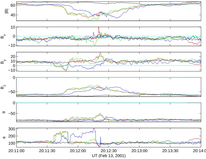
40 60 |B| −10 0 10 B x −10 0 10 20 B y −50 0 B z −50 0 θ 20:11:00 20:11:30 20:12:00 20:12:30 20:13:00 20:13:30 20:14:00 100 200 300 φ UT (Feb 13, 2001)
Fig. 9. FGM data in the interval 20:11–20:14. The format is the same as Fig. 6.
indicates that the boundary is also tilted. This is consistent with the spacecraft entering through the duskward side of an indented structure as the boundary moves dawnwards, psumably in response to the y-component of the IMF. A re-markable feature of the entry as seen by spacecraft 2–4 is that even with the highest resolution data, the By rotation
occurs in different orders at the three spacecraft throughout cusp entry. This implies very fine-scale structure in the field at this time. The conjectured nature of the outer boundary (labelled A) is shown in more detail at the top right. The z component of the magnetic field is roughly unchanged across the boundary, but the y-component is shut off, hence leading to the field depletion.
4.2 Cusp interior and exit
When spin-averaged data is considered, the field within the cusp shows a reasonable correlation between the three trail-ing spacecraft, but with no obvious correlation between these and the leading spacecraft. However, the high resolution data shows a lack of any correlation even between the trail-ing three spacecraft, as can be seen, in particular, around
20:03 UT in Fig. 6. The field is also very unsteady (δB/B of order unity). The turbulence in the cusp is very different to that seen in the magnetosheath, which appears to be the usual mirror modes. A fuller study of cusp turbulence will be presented elsewhere.
The cusp exit corresponds to the interval 20:06:30– 20:08:30. An examination of the right-hand side of Fig. 6 shows that spacecraft 1 exits first, through a boundary that lasts 15 s, consisting of a smooth increase in Bzwith a small
rotation of By. Mapping this boundary to the other three
spacecraft would result in spacecraft 4 exiting next, followed by spacecraft 2 and 3. Spacecraft motion of −2.7 km/s in the x-direction would lead to delays of 160 s to spacecraft 4, and 70 s thereafter to spacecraft 2 and 3. However, the sharp boundary seen by spacecraft 1 is replaced by a more diffuse structure, which for spacecraft 2 and 3 commences at the same time as the boundary seen by spacecraft 1, but lasts 90 s.
We first analyse the exit seen by spacecraft 1. For the interval corresponding to the principal boundary (20:06:30–20:07:30), a MVA analysis gives a “good” normal
component of −2 nT and a normal velocity of −33 km/s. We stress that for all intervals considered the normal field component was small (3 nT or less) and negative. The rear boundary of the cusp is thus oriented almost exactly in the y–z plane, and has a weak field component passing tailward through it, implying that it may not be a tangential disconti-nuity. However, we were unable to find a good deHoffman-Teller frame. Analysis of data from the other three spacecraft does not reveal any reliable minimum variance directions, despite a search over many intervals.
If we assume that the cusp exit at spacecraft 1 begins at 20:07:54, and the exit at spacecraft 2–4 at 20:08:03, then the cusp edge is moving in the +x direction at 35 km/s (where the satellite motion is included). However, the cusp boundary clearly changes in the few seconds between the crossings of spacecraft 1 and 2 from a sharp jump to a more diffuse struc-ture. One scenario for the very broad transition is that the rear boundary of the cusp is retreating at almost exactly the speed of the spacecraft (i.e. 2.7 km/s). This is not inconsistent with the order 4–(3,2) in which the three spacecraft encounter the diffuse part of the boundary, but is difficult to understand given the synchronism of the initial boundary encounter of the three trailing spacecraft with that seen by spacecraft 1. An alternative explanation could be that the initially sharp boundary suddenly undergoes a relaxation and expands back-wards: the magnetic field profile is perhaps reminiscent of a rarefaction wave.
This boundary is also evident in the CIS data. The density seen by spacecraft 1 undergoes an abrupt decrease by a factor of 2 on the same time scale as the field, while the density at spacecraft 3 decreases more gently, also on a similar scale to the field. Similar remarks apply to the temperature, and we note that the magnitude of Vzdecreases across the boundary.
This is also not inconsistent with a propagating rarefaction wave. The lower part of Fig. 8 shows this boundary (labelled B), and its relative orientation with respect to both the nomi-nal magnetopause and the cusp entry. At the top left we show schematically how the magnetic field and solar wind plasma behave there. The z magnetic field is compressed by roughly a factor of two, while plasma streams tailward through the boundary.
4.3 Trailing cusp signatures
At 20:12, FGM on spacecraft 2–4 detects a brief cusp en-counter seen in Fig. 4. At this time spacecraft 1, which is leading, sees a smooth background field: Fig. 9 shows the high resolution magnetic fields in the immediate vicinity of this encounter. The obvious interpretation is that this is a back and forth motion of the cusp that moves over spacecraft 2–4, but does not reach spacecraft 1. However, a closer ex-amination of the data suggests that this is not the case. A back and forth motion would reveal a nested structure in the time series as the spacecraft closest to the cusp (i.e. 2 and 3) had entered it first, and left it after spacecraft 4. In fact, what Fig. 9 indicates is that this apparent cusp re-entry is in fact
4 both enters and leaves the field depletion (which is evident predominately in Bz)after spacecraft 2 and 3. We also note
that the minimum variance direction here was approximately in the x direction.
An examination of the CIS data around the third black line in Fig. 4 reveals that the field depletion has no obvious sig-nature in the density at either spacecraft 1 or 3, but there is a clear temperature enhancement at spacecraft 3, but not at spacecraft 1. In other words, the plasma here is cusp-like. However, just following the field pulse, the temperature at spacecraft 1 also increases at 20:15, and spacecraft 1 and 3 see broadly the same enhanced temperature profile through the next few minutes. This region (20:12–20:18) is also as-sociated with significant fluctuations in By (a few nT) that
are reasonably coherent at spacecraft 2–4, but are totally dif-ferent at spacecraft 1. We interpret this as being residual cusp turbulence moving over the spacecraft, and being asso-ciated with hot cusp-like plasma. It is also interesting to note that there is a further spell of perpendicular heating between 20:25 and 20:30, seen first by spacecraft 3, then by spacecraft 1. This has no obvious field signature. Such global tem-perature changes are often observed in the cusp and plasma mantle regions (Lavraud et al., 2004) and are associated with large-scale changes in the ion energy distributions.
These observations can be interpreted in a number of ways. One is that the rear boundary of the cusp is intrin-sically unstable, and detaches pulses of cusp-like plasma which then move tailwards. A second possibility is that the rear of the cusp responds to changes in the magnetic merging process elsewhere on the magnetopause by breaking up and reforming. In this context we note the reversal of Byat 20:10
(Fig. 3). Clearly either process is confined to the upper part of the exterior cusp, since spacecraft 1, being deeper in the magnetosphere, does not see these signatures. It is also pos-sible the highly variable cusp structure at 20:07–20:08 is an earlier manifestation of such processes. Plasma associated with these detachments streams along the field lines, passing over the spacecraft, first 3, then 1. Thus, the plasma extent of the detachments is larger than that associated with the field. After 20:30, Cluster is too far from the magnetopause to see any evidence of the detachments, which are thus a local phe-nomenon.
5 The cusp crossing of 20 February 2001
One week later, at 23:30 UT on 20 February 2001, Cluster encountered the cusp in an apparently very similar manner, with a clear entry through the magnetopause and exit through the cusp rear boundary. While the data coverage is somewhat more limited, this crossing is especially interesting as it oc-curs during a magnetic field conjunction of Cluster and the FAST spacecraft. The full details of this encounter will be presented elsewhere, so we now only present the similari-ties and differences with the crossing of 13 February. The
0 5 10 |B|(nT) −5 0 5 B x −50 5 10 B y −5 0 5 10 B z 0 5 10 n(cm −3 ) 300 350 400 v(km/s) 22:000 22:15 22:30 22:45 23:00 23:15 23:30 23:45 00:00 1 2 P D (nPa)
20 February (UT): GSE lagged
Fig. 10. Data from the ACE spacecraft located in the solar wind between 22:00 and 23:59 on 20 February 2001. A constant lag speed of
350 km/s has been used. The format is the same as Fig. 3.
satellite configuration is effectively the same as in Fig. 2, but displaced by roughly 1 REin the GSE–y direction.
A significant difference was in the solar wind conditions. Figure 10 shows the lagged IMF and solar wind plasma quan-tities from 22:00 to 23:59 on 20 February. The slow solar wind speed leads to a long lag time of 1 h 20 min. At the time of the cusp encounters (23:20–23:35), the solar wind density is low, and the dominant magnetic field component is in the -y direction. Bz turned southward at 23:10 and
re-mained in that direction until the end of 20 February. The southward IMF is slightly weaker than on 13 February, but the solar wind speed is diminished considerably, so that one might expect a lower level of magnetopause reconnection. The various indices confirm that this was a time of low geo-magnetic activity with Dst= 0 nT and Kp=1.5.
Figure 11 shows a summary of the crossing in the same form as Fig. 4 between 23:00 and 23:59. We identify four boundaries, as shown by the solid vertical lines. The cusp is a clearly identifiable structure in the magnetic field, commenc-ing at 23:20 UT and endcommenc-ing at 23:32 UT (outer two lines).
The x-magnetic field component is close to zero throughout much of the passage. In the magnetosheath the dominant field component is in the -y direction, as expected from the IMF. Cusp entry occurs for all spacecraft at around 23:20, but is preceded by a large positive rotation of By, and
ad-justment of Bz such that the total field magnitude remains
constant. This is similar to what was seen prior to cusp entry on 13 February, but on this occasion we believe it is directly associated with cusp entry. Given the constancy of the IMF Byat this time, it is unlikely to be an effect due to a mapping
of the IMF to the cusps, and, unlike on 13 February, there are no major Byexcursions in the magnetosheath in the
preced-ing three hours. This rotation can also be associated with an enhancement of temperature by a factor of three (last panel of Fig. 10): again this differs from the 13 February case. We also note that there appears to be a brief re-entry into the magnetosheath between 23:25 and 23:26, as indicated by the inner two solid lines. The cusp exit is clearly seen in the field at 23:33, after which time Cluster is in the plasma mantle region.
20 40 |B|(nT) −40 −20 0 20 40 B y (nT) −40 −200 20 40 B z (nT) 10 20 30 n p (cm −3 ) −300 −200 −100 0 100 V (km/s) 23:00 23:05 23:10 23:15 23:20 23:25 23:30 23:35 23:40 23:45 2 4 6 T(MK) 20 Feb 2001 (UT)
Fig. 11. An overview of the magnetic field and plasma parameters between 23:00 and 23:45 UT on 20 February 2001. The six panels show |B|, ByBz, n, V and T. The three components of the plasma velocity seen by spacecraft 1 are denoted by cyan, red and magenta lines in
panel 5. The four vertical lines refer to features discussed in the text.
There is no discernible change in the density at any of the crossings into and out of the cusp, and no rapid density decrease as the spacecraft exit the cusp into the magneto-sphere, but the density falls off rapidly after 23:50. This is also evident from CIS spectrograms (not shown) which show a gentle decline in solar wind plasma towards 23:50 UT. The magnetosheath plasma is seen to be flowing towards the tail, but the abrupt change in Byat cusp entry is associated with
a strong, negative flow in the y direction, which also cor-responds to the onset of proton heating. PEACE data (not shown) shows that solar wind electrons are seen at all 4 spacecraft, with an abrupt cutoff at 23:50, similar to the ions. We now focus on the cusp as seen by the four FGM instru-ments. Figure 12 shows the magnetic field between 23:15 and 23:40, using data with 4 vectors per second. The transi-tion through the cusps involves a partial entry of all space-craft into the cusp (23:18–23:21), followed by an exit of spacecraft 2–4 back into the magnetosheath (23:21–23:25), at which time spacecraft 1 also re-enters the magnetosheath.
All four spacecraft then enter the cusp at 23:26, and exit into the plasma mantle at 23:33. All of these features are seen best in By, with strong negative values of Bybeing identified
as being the magnetosheath. (We note here such an inter-pretation may have problems since the ion temperature does not revert to its magnetosheath value.) The time over which all spacecraft are in the cusp is 5–6 min, very similar to that on 13 February. On this occasion, we see no evidence for trailing magnetic features.
We carried out a MVA analysis of cusp entry and exit. For the interval 23:17–23:21 of cusp entry, we were unable to find good eigenvalues (λ3/λ1>10), despite a search over
many data intervals. For spacecraft 1–4, the ratios are 5.7, 5.6, 5 and 3.8 (see also Dunlop et al., 2004), but for the record we state the four spacecraft average normal as n=(0.99,
−0.06, −0.14). The average normal field over the four spacecraft is 0.94 nT (i.e. outwards), with a normal flow of
−46 km/s (inwards). While we can find a good deHoffman-Teller frame (correlation 0.94), the Walen relations are not
20 40 |B| −20 0 20 B x −40 −20 0 20 40 B y −40 −20 0 20 40 B z −50 0 50 θ 23:15 23:17 23:19 23:21 23:23 23:25 23:27 23:29 23:31 23:33 23:35 100 200 300 φ UT (Feb 20, 2001)
Fig. 12. The magnetic field with a resolution of 4 vectors per second from 23:15–23:35 UT on 20 February 2001. The six panels show the
magnetic field magnitude, components and orientations (expressed as the angles θ and φ) in GSE coordinates.
satisfied (the best slope is 0.4). At cusp exit, the search for “good” normals proved fruitless.
An examination of the four boundaries is revealing. The first cusp entry involves the sequence 1–3–4–2 into the By
rotation, but 3–2–1–4 through the decrease in field magni-tude. To put these and subsequent results in context, motion through a planar boundary would lead to spacecraft 1 lead-ing the others by approximately 3 min. Instead, the order of boundary crossings between 23:20 and 23:29 has spacecraft 3 leading on each occasion, more suggestive again of a side-ways motion of the cusp-magnetosheath boundary, as in the 13 February encounter.
Thus, for a case with entirely different IMF properties (quiet solar wind, strong By), the cusp field and plasma
struc-ture has similarities to that on the disturbed 13 February 2001. There is a clear “magnetic cusp”, with very abrupt boundaries, and a plasma cusp that is simply a diffuse ex-tension of the solar wind, and indicates ready access of solar wind plasma into and beyond the magnetic cusp.
6 Summary and discussion
We have examined two cusp crossings from the first year of the Cluster mission when the spacecraft separation was of the order of 600 km. Unlike other cases examined by Lavraud et al. (2002, 2004), which showed evidence for large regions of stagnant plasma, these cusp crossings are rather brief en-counters, dominated by tailward-flowing plasma. In both cases the IMF was southward, leading to the expectation of an open magnetosphere.
In the case of 13 February 2001, where we were able to carry out a valid analysis of the normals of the cusp bound-ary, it was shown that the boundary between the magne-tosheath and cusp had both a normal component of field and plasma flow through it, although the Walen relations, which would indicate a rotational discontinuity, were not definitively satisfied. This boundary should be thought of as the magnetopause, since it marks a clear transition be-tween the solar and terrestrial magnetic field components. The cusp exit was through another open boundary, albeit
plasma streaming tailward into the magnetosphere. Although a multiple boundary cusp structure for southward IMF has been proposed by Vasyliunas (1995), we note that there are some differences between his suggestions and the findings of the present paper, especially in the magnetic structure of the innermost boundary.
Evidence was found for instability of the cusp on one occa-sion, and it was clear from multi-spacecraft analysis that the cusp boundary itself is highly dynamic, both moving from point to point, and changing width on very short time scales. This is of course not unexpected, since the cusp is a region where plasma and magnetic pressures are similar, so that small changes in the solar wind dynamic pressure may have a large effect. The case of 20 February showed a similar cusp duration, but here the spacecraft underwent a complex series of entries into and out of the cusp. It is striking that very sim-ilar field and plasma profiles were seen for two distinct IMF conditions.
How do these results fit in with others obtained from Clus-ter? It is very clear that we are seeing a different cusp to that reported elsewhere by Lavraud et al. (2002, 2004). First, given the nature of the inbound orbit, it is likely that we are seeing the very tailward part of the exterior cusp, as op-posed to the more extended region reported in those papers. In addition, while Lavraud et al. (2002) reported a stagnant region under northward IMF conditions, the present study indicates that the exterior cusp is largely convective under the present southward IMF conditions. This differing be-haviour is compatible with the inferred magnetic topology and plasma flow properties expected from lobe and sub-solar reconnection processes for northward and southward IMF, respectively. Further clarification of the global geometry re-quires an extensive survey of Cluster data at all spacecraft separations.
Acknowledgements. Work in the UK and France was supported by PPARC and CNES. PC acknowledges support of a PPARC senior research fellowship. DLH acknowledges support from NASA grant NAG5-9584. ACE data was obtained from the ACE Science Center, CalTech. We thank the referee for helpful comments.
Topical Editor T. Pulkkinen thanks N. Maynard for his help in evaluating this paper.
References
Balogh, A., Dunlop, M. W., Cowley, S. W. H., et al.: The Clus-ter magnetic field investigation, Space Sci. Rev., 79, (5), 65–91, 1997.
Balogh, A., Carr, C. M., Acuna, M. H., et al.: The Cluster magnetic field investigation: overview of in-flight performance and initial results, Ann. Geophys., 19, 1207–1217, 2001.
Cargill, P. J., Dunlop, M. W., Balogh, A., and the FGM team: First Cluster-II results of the magnetic field structure of the medium and high-altitude cusps, Ann. Geophys., 19, 1533–1544, 2001. Chang, S.-W., Scudder, J. D., Fennell, J. F., et al.: Energetic
mag-netosheath ions connected to the Earth’s bow shock: Possible
2000.
Chen, J. S. and Fritz, T. A.: Correlation of cusp MeV helium with turbulent ULF power spectra and its implications, Geophys. Res. Lett., 25, 4113–4116, 1998.
Crooker, N. U.: Dayside merging and cusp geometry, J. Geophys. Res., 84, 951–959, 1979.
Dungey, J. W.: Interplanetary magnetic field and the auroral zones, Phys. Rev. Lett., 6, 47–48, 1961.
Dungey, J. W.: Adventures in velocity space, in Geophysics: The Earth’s environment, edited by Dewitt, C., Hieblot, J., and Lebeau, A., Gordon and Breach, 551–603, 1963.
Dunlop, M. W., Cargill, P. J., Stubbs, T. J., and Woolliams, P.: The high altitude cusps: HEOS-2, J. Geophys. Res., 105, 27 509– 27 518, 2000.
Dunlop, M. W., Balogh, A., and Glassmeier, K.-H.: Four-point clus-ter application of magnetic field analysis tools: The discontinu-ity analyser, J. Geophys. Res., 107, doi:10.1029/2001JA005089, 2002.
Dunlop, M. W., Lavraud, B., Cargill, P. J., et al.: Cluster observa-tions of the cusp: magnetic structure and dynamics, Surveys in Geophysics, in press, 2004.
Eastman, T. E., Boardsen, S. A., Chen, S.-H., and Fung, S. F.: Con-figuration of high-latitude and high-altitude boundary layers, J. Geophys. Res., 105, 23 221–23 238, 2000.
Elphic, R. C., Dunlop, M. W., Balogh, A., et al.: Transient recon-nection as observed in the cusp by Cluster and FAST, EOS Trans. AGU, 82, (47), Fall Meet. Supp., Abstract SM12C-07, 2001. Farrell, W. M. and van Allen, J. A.: Observations of the Earth’s
polar cleft at large radial distances with the Hawkeye 1 satellite, J. Geophys. Res., 95, 20 945–20 958, 1990.
Fritz, T. A., Chen, J., and Siscoe, G. L.: Energetic ions, large dia-magnetic cavities, and Chapman-Ferraro cusp, J. Geophys. Res., 108, SMP 17, doi:10.1029/2002JA009476, 2003.
Grande, M., Fennell, J., Livi, S., et al.: First polar and 1995–034 ob-servations of the mid-altitude cusp during a persistent northward IMF condition, Geophys. Res. Lett, 24, 1475–1478, 1997. Kessel, R. L., Chen, S. H., Green J. L., et al.: Evidence of
high-latitude reconnection during northward IMF: Hawkeye observa-tions, Geophys. Res. Lett, 23, 583–586, 1996.
Khrabrov, A. V. and Sonnerup, B. U. ¨O.: DeHoffmann-Teller anal-ysis, in analysis methods for multispacecraft data, ISSI Scientific Report SR-001, ESA Publications, Noordwijk, The Netherlands, 221–247, 1998.
Lavraud, B., Dunlop, M. W., Phan, T., et al.: Properties, struc-ture and dynamics of the stagnant exterior cusp: CLUSTER first results, Geophys. Res. Lett., 29, doi:10.1029/2002GL015464, 2002.
Lavraud, B., Reme, H., Dunlop, M. W., et al.: Cluster observes the high altitude/exterior cusp regions, Surveys in Geophysics, in press, 2004.
Maynard, N. C., Burke, W. J., Sandholt, P. E., et al.: Observations of simultaneous effects of merging in both hemispheres, J. Geo-phys. Res., 106, 24 551–24 577, 2001.
Merka, J., Safrankova, J., Nemecek, Z., Savin, S., and Skalsky, A.: High altitude cusp: INTERBALL observations, Adv. Space. Res, 25, (7/8), 1425–1434, 2000.
Paschmann, G., Haerendel, G., Sckopke, N., and Rosenbauer, H.: Plasma and magnetic field characteristics of the distant polar cusp near local noon: The entry layer, J. Geophys. Res., 81, 2883–2899, 1976.
R`eme, H., Aoustin, C., Bousqued, J.-M., et al.: First multispacecraft ion measurements in and near the Earth’s magnetosphere with the identical cluster ion spectrometry (CIS) experiment, Ann. Geo-phys., 19, 1303–1354, 2001.
Sandahl, I., Popielawska, B., Budnick, E. Y., Fedorov, A., Savin, S., Safrankova, J., and Nemecek, Z.: The cusp as seen from interball, in Proc. Cluster-II workshop on multiscale/multipoint plasma measurements, ESA SP-449, 39–45, 2000.
Scudder, J. D., Mozer, F. S., Maynard, N. C., and Russell, C. T.: Fingerprints of collisionless reconnection at the separator, J. Geophys. Res., 107, doi:10.1029/2001JA000126, 2002. Sonnerup, B. U. ¨O. and Scheible, M.: Minimum and maximum
variance analysis, in analysis methods for multispacecraft data, ISSI Scientific Report SR-001, ESA publications, Noordwijk, The Netherlands, 185–219, 1998.
Stubbs, T. J., Lockwood, M., Cargill, P. J., Fennel, J., Grande, M., Kellett, B., Perry, C., and Rees, A.: Dawn/dusk asymmetry in particles of solar wind origin within the magnetosphere, Ann. Geophys., 19, 1–9, 2001.
Tsyganenko, N. A.: A magnetospheric magnetic field model with a warped tail current sheet, Planet. Space Sci., 37, 5–20, 1989. Vasyliunas, V. M.: Multiple-branch model of the open
magne-topause, Geophys. Res. Lett., 22, 1145–1147, 1995.
Vontrat-Reberac, A., Bousqued, J.-M., Taylor, M. G. G. T., et al.: Cluster observations of the high-altitude cusp for northward in-terplanetary magnetic field: a case study, J. Geophys. Res., 108, doi:10.1029/2002JA001717, 2003.
Zhou, X. W. and Russell, C. T.: The location of the high latitude polar cusp and the shape of the surrounding magnetosphere, J. Geophys. Res., 102, 105–110, 1997.