Mixed-Integer Programming Approaches for Hydropower Generator Maintenance Scheduling

MIXED-INTEGER PROGRAMMING APPROACHES FOR HYDROPOWER GENERATOR MAINTENANCE SCHEDULING

JESÚS ANDRÉS RODRÍGUEZ SARASTY

DÉPARTEMENT DE MATHÉMATIQUES ET DE GÉNIE INDUSTRIEL ÉCOLE POLYTECHNIQUE DE MONTRÉAL

THÈSE PRÉSENTÉE EN VUE DE L’OBTENTION DU DIPLÔME DE PHILOSOPHIÆ DOCTOR

(MATHÉMATIQUES DE L’INGÉNIEUR) AOÛT 2018

ÉCOLE POLYTECHNIQUE DE MONTRÉAL

Cette thèse intitulée :

MIXED-INTEGER PROGRAMMING APPROACHES FOR HYDROPOWER GENERATOR MAINTENANCE SCHEDULING

présentée par : RODRÍGUEZ SARASTY Jesús Andrés en vue de l’obtention du diplôme de : Philosophiæ Doctor a été dûment acceptée par le jury d’examen constitué de :

M. GENDREAU Michel, Ph. D., président

M. ANJOS Miguel F., Ph. D., membre et directeur de recherche M. DESAULNIERS Guy, Ph. D., membre et codirecteur de recherche M. CORDEAU Jean-François, Ph. D., membre

DEDICATION

ACKNOWLEDGEMENTS

First, I would like to express my gratitude to my research supervisor, Professor Miguel Anjos, for all the advice, the positive feedback, the interesting discussions, and for giving me the opportunity to develop my research interests during this PhD. I thank him for his vote of confidence and for supporting my engagement in the industrial project that motivated this dissertation.

I am also thankful to my research co-supervisor, Professor Guy Desaulniers, for his insightful comments, his thorough reviews, and his advice about the completion of my PhD. My gra-titude also to Professor Charles Audet for his involvement in the initial stage of the project. Special thanks to Dr. Pascal Côté for his invitation to work on this project, and for his participation as an industrial co-supervisor. His support was crucial for achieving the project goals. Thanks to Bruno Larouche and Jean-François Gauthier of Rio Tinto Aluminium for endorsing the financial support of the company during the 22 months of the project.

This research was also supported by grants of NSERC Engage and MITACS Accelerate pro-grams. I also thank the Fields Institute of Mathematics of the University of Toronto, for sponsoring a poster presentation about this research at the Workshop on Nonlinear Optimi-zation Algorithms and Industrial Applications, in Toronto, June 2016.

Thanks to the support team of GERAD (Marie, Pierre, Logo, Marilyne) and to the Énergie Électrique group of Rio Tinto in Saguenay, for providing a propitious environment for this research. Special thanks to Christophe Tribes for his assistance to set up the compilation directives for the code of this project at GERAD.

This research was motivated by an industrial problem presented at the Sixth Industrial Problem Solving Workshop, in August 2015, at the University of Montreal. I thank the organizers of that event and the Centre de Recherches Mathématiques of the University of Montreal, for creating opportunities to connect industrial problems with research in academia.

RÉSUMÉ

Dans les systèmes de production d’électricité, la maintenance régulière des unités de produc-tion est essentielle pour éviter des pannes imprévues et coûteuses, pour maintenir l’efficacité du système et pour prolonger la durée de vie de l’équipement. Cependant, l’arrêt des gé-nérateurs pour maintenance préventive réduit temporairement la capacité, l’efficacité et la fiabilité du système.

Etant donnée une liste des activités de maintenance à réaliser dans un horizon de planifica-tion, le problème de planification de maintenance des générateurs (GMSP, pour Generator Maintenance Scheduling Problem) consiste à déterminer un calendrier d’arrêts pour mainte-nance qui maximise une métrique de performance du système. Le calendrier optimal qui en résulte doit répondre aux exigences opérationnelles de la production d’électricité ainsi qu’aux contraintes de maintenance, telles que les fenêtres de temps des activités de maintenance. Dans les systèmes hydroélectriques, l’ordonnancement de la maintenance des unités de pro-duction comporte des défis uniques en raison de la non-linéarité de la propro-duction d’hydro-électricité, de l’incertitude des débits d’eau et de l’interdépendance des décisions opération-nelles dans l’espace et le temps. Le GMSP est particulièrement pertinent pour les producteurs d’hydroélectricité parce que l’avancement ou le report des activités de maintenance peut générer des économies significatives en réduisant les déversements d’eau et en améliorant l’efficacité de la production d’hydroélectricité.

Nous développons un programme linéaire mixte en nombres entiers (MILP, pour Mixed-Integer Linear Program) pour le GSMP dans les systèmes hydroélectriques, avec hyperplans pour approximer l’effet non-linéaire des rejets d’eau, les niveaux d’eau stockés et le nombre de générateurs actifs sur la production d’hydroélectricité. Nous affinons notre formulation en utilisant des inégalités valides, la désagrégation de variables et de contraintes, et une technique de réduction de modèle basée sur des informations de fenêtres temporelles. Nos tests numériques montrent que la meilleure combinaison de ces techniques peut réduire jusqu’à dix fois le temps de calcul pour obtenir une solution.

Pour incorporer l’effet des afflux d’eau incertains, nous étendons notre modèle en un pro-gramme linéaire stochastique en deux étapes, et nous implémentons une méthode de décom-position de Benders parallélisée pour sa solution. Nous proposons sept techniques d’accélé-ration, et lors de nos expériences numériques, nous observons qu’une combinaison de cinq de ces techniques permet d’obtenir les meilleures performances, avec une accélération de l’algo-rithme de Benders quadruplée par rapport à la méthode Benders de base. Nos tests sur une

grille de calcul avec 200 cœurs pour résoudre le problème avec un grand nombre de scénarios, confirment la supériorité de la méthode Benders parallélisée par rapport à la solution directe avec un solveur général pour MILP.

Enfin, nous proposons des extensions de notre formulation, en incluant d’autres contraintes de maintenance pertinentes, des décisions sur la durée des activités et des réserves de production pour anticiper l’incertitude de la charge d’électricité. En outre, nous présentons d’autres stra-tégies de décomposition pour les GMSP dans les systèmes hydroélectriques et nous discutons des perspectives de recherche, telles que des améliorations à la méthode de décomposition et les applications de notre formulation MILP à des problèmes d’ordonnancement similaires.

ABSTRACT

In power generation systems, regular maintenance of generating units is essential to prevent costly unplanned outages, to sustain the efficiency of the system, and to extend the lifespan of the equipment. However, shutting down generators for preventive maintenance temporarily reduces the capacity, efficiency, and reliability of the system.

Given a list of maintenance activities to be completed within a planning horizon, the Gen-erator Maintenance Scheduling Problem (GMSP) is to determine a calendar of maintenance outages that maximizes a system performance metric. The resulting optimal schedule must meet operational requirements of the electricity production, as well as maintenance con-straints, such as time windows of maintenance activities.

In hydropower systems, maintenance scheduling of generating units entails unique challenges due to the nonlinearity of the hydroelectricity production, the uncertainty of the water inflows and the interdependence of operational decisions in space and time. The GSMP is particularly relevant for hydropower producers because advancing or postponing maintenance activities can yield significant savings by reducing water spills and improving the efficiency of the hydroelectricity production.

We develop a compact Mixed-Integer Linear Program (MILP) for the GSMP in hydropower systems, with hyperplanes for approximating the nonlinear effect of the water discharges, the stored water levels and the number of active generators on the hydroelectricity production. We refine our formulation using valid inequalities, disaggregation of variables and constraints, and a model reduction technique based on time windows information. In computational experiments, we find that the best combination of such tightening techniques can reduce the computational time of the solution by up to one order of magnitude.

To incorporate the effect of uncertain water inflows, we extend our model as a two-stage stochastic linear program, and we implement a parallelized Benders decomposition method for its solution. We implement seven acceleration techniques, and through computational ex-periments, we find that a combination of five of such techniques achieves the best performance with a fourfold speedup of the Benders algorithm. Our tests on a 200-core computer cluster for solving the problem with a large number of inflow scenarios, confirm the superiority of the parallelized Benders method over the direct solution with a general MILP solver.

Finally, we outline extensions to our formulation, by including other relevant maintenance constraints, decisions on the duration of activities, and generation reserves to buffer the

un-certainty of the electricity load. Furthermore, we outline alternative decomposition strategies for the GSMP in hydropower systems and we discuss directions of future research, such as en-hancements to the decomposition method and applications of our compact MILP formulation to similar scheduling problems.

TABLE OF CONTENTS DEDICATION . . . iii ACKNOWLEDGEMENTS . . . iv RÉSUMÉ . . . v ABSTRACT . . . vii TABLE OF CONTENTS . . . ix

LIST OF TABLES . . . xii

LIST OF FIGURES . . . xiii

LIST OF SYMBOLS AND ABBREVIATIONS . . . xv

CHAPTER 1 INTRODUCTION . . . 1

1.1 Maintenance planning and scheduling . . . 1

1.2 Challenges of maintenance scheduling in hydropower systems . . . 2

1.3 Purpose of this study . . . 4

1.4 Main contributions . . . 5

1.5 Plan of the dissertation . . . 6

CHAPTER 2 LITERATURE REVIEW . . . 7

2.1 Basic concepts of mixed-integer linear programming . . . 7

2.1.1 General exact solution methods for mixed-integer linear programs . . 8

2.1.2 Decomposition methods for mixed-integer programs . . . 10

2.1.3 Benders decomposition . . . 13

2.1.4 Stochastic programming . . . 17

2.2 Generator maintenance scheduling in hydropower systems . . . 19

2.2.1 Planning and operation of hydropower systems . . . 19

2.2.2 Generator maintenance scheduling . . . 20

2.2.3 Maintenance scheduling of generating units in hydropower systems . . 21

CHAPTER 4 ARTICLE 1: MILP FORMULATIONS FOR GENERATOR

MAINTE-NANCE SCHEDULING IN HYDROPOWER SYSTEMS . . . 28

4.1 Notation . . . 28

4.2 Introduction . . . 30

4.3 A basic mixed integer programming formulation . . . 33

4.3.1 The hydropower operation . . . 33

4.3.2 Linearization of the power production function . . . 35

4.3.3 The maintenance scheduling problem . . . 37

4.3.4 The objective function . . . 38

4.3.5 The complete basic model . . . 38

4.4 Tightening approaches . . . 39

4.4.1 Extended formulation . . . 39

4.4.2 Set reduction . . . 40

4.4.3 Valid inequalities . . . 41

4.5 Computational experiments . . . 42

4.5.1 Computational results for all formulations . . . 43

4.5.2 Optimality gaps of the best formulations . . . 45

4.6 Industrial application . . . 47

4.7 Conclusions . . . 48

4.8 Appendices . . . 49

4.8.1 Appendix A: Proof of proposition 1 . . . 49

4.8.2 Appendix B: Proof of proposition 2 . . . 49

4.8.3 Appendix C: Proof of proposition 3 . . . 50

CHAPTER 5 ARTICLE 2: STOCHASTIC HYDROPOWER GENERATOR MAIN-TENANCE SCHEDULING VIA BENDERS DECOMPOSITION . . . 52

5.1 Introduction . . . 52

5.2 Mathematical programming models . . . 55

5.2.1 Two-stage stochastic programming approach . . . 55

5.2.2 Mathematical program . . . 57

5.3 Solution strategy . . . 59

5.3.1 The Benders decomposition method . . . 60

5.3.2 Benders reformulation of the SGMSP . . . 61

5.4 Acceleration techniques for Benders decomposition . . . 64

5.4.1 Implemented techniques . . . 65

5.5 Computational experiments . . . 72

5.5.1 Selection of acceleration techniques . . . 72

5.5.2 Effect of parallelization . . . 75

5.6 Conclusions and future work . . . 76

5.7 Acknowledgments . . . 78

5.8 Appendices . . . 78

5.8.1 Appendix A: Model supplement . . . 78

5.8.2 Appendix B: Selecting multiple-phase relaxation sequence and valid inequalities . . . 81

5.8.3 Appendix C: Nomenclature . . . 84

CHAPTER 6 EXTENSIONS . . . 87

6.1 Model extensions . . . 87

6.1.1 Additional maintenance constraints . . . 87

6.1.2 Selecting the duration of maintenance activities . . . 90

6.1.3 Load uncertainty and generation reserves . . . 91

6.2 Alternative Decomposition Strategy (ADS) . . . 94

CHAPTER 7 GENERAL DISCUSSION . . . 101

7.1 Synthesis of work . . . 101

7.1.1 MILP formulations for SGMSP . . . 105

7.1.2 Decomposition methods for SGMSP . . . 106

7.2 Study limitations and future research . . . 108

7.2.1 Model extensions . . . 108

7.2.2 Refinements to the implemented solution methods . . . 109

7.2.3 Sub-decomposition approach . . . 109

CHAPTER 8 CONCLUSION AND RECOMMENDATIONS . . . 111

LIST OF TABLES

3.1 Summary of thesis organization . . . 27

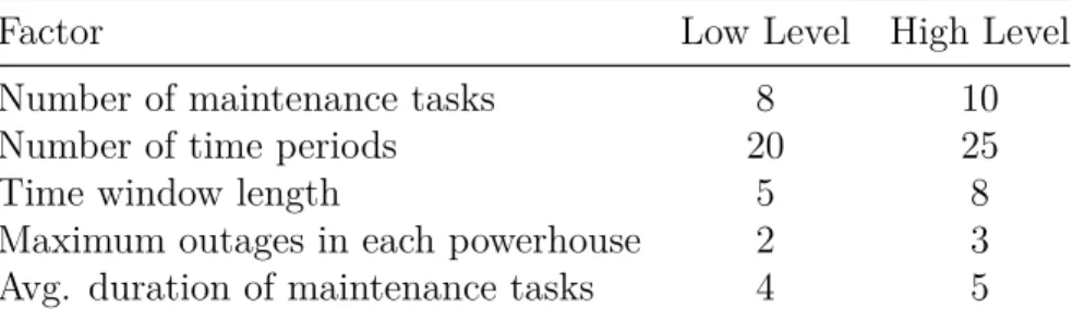
4.1 Levels of factors of test intances to compare all formulations . . . 43

4.2 Normalized log CPU times per instance . . . 44

4.3 p-values based on normalized log CPU time . . . 45

4.4 Levels of factors of test instances to compare the best formulations . 46 4.5 Optimality gap statistics . . . 47

4.6 Basic attributes of the hydropower system . . . 47

5.1 Configuration of relaxation levels . . . 67

5.2 Sequences of relaxation levels for multi-phase relaxation . . . 67

5.3 Basic attributes of the hydropower system . . . 73

5.4 Summary statistics of the acceleration methods applied independently 74 5.5 Summary of linear regression model with techniques VI, MP, CC and IRC as main factors . . . 75

5.6 Summary of linear regression model with factors CC and IRC and interaction term . . . 75

5.7 Statistics on the computational times with parallel Benders decomposi-tion and MILP-based soludecomposi-tion, with different numbers of inflow scenarios 77 5.8 Mean, standard deviation and 95 % confidence interval of the objective function values . . . 78

5.9 Summary of ANOVA with valid inequalities 1, 2 and 3 as main factors, and normalized computational time as response variable. . . 82

5.10 Summary of ANOVA with valid inequalities 1 and 2 and interaction term, and normalized computational time as response variable. . . 82

5.11 Parameters of stages in multi-phase relaxation. . . 82

5.12 Summary statistics of normalized computational times of multi-phase relaxations . . . 83

6.1 Computational time and relative optimality gap of two parallel Benders and ADS . . . 100

7.1 Summary of contributions I . . . 102

7.2 Summary of contributions II . . . 103

LIST OF FIGURES

1.1 Schematic of a hydroelectric powerhouse . . . 2

1.2 Hydroelectricity production function of a generating unit . . . 3

1.3 Mass balance in a reservoir . . . 3

1.4 Time series of 11 forecasted water inflow scenarios . . . 4

1.5 Schematic of generator maintenance scheduling in hydropower systems 5 2.1 Graphical solution to a linear program . . . 8

2.2 Graphical solution to a linear integer program . . . 9

2.3 Linear relaxation solution to an linear integer program after branching on a fractional variable . . . 10

2.4 Flow diagram of the Benders decomposition method . . . 15

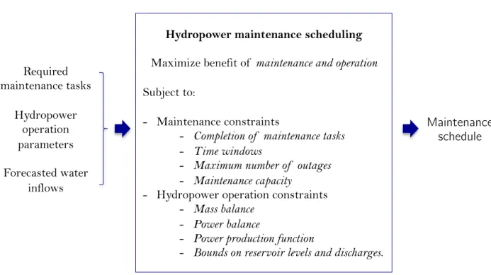
3.1 Input-output diagram of the hydropower maintenance scheduling prob-lem . . . 25

4.1 Maximum power output as a function of water discharge and stored water and number of active generators . . . 31

4.2 Timeline for a maintenance activity m. . . . 40

4.3 Performance profiles of the tested formulations . . . 46

5.1 Maximum power generation in a powerhouse, for different values of u, s and k . . . 53

5.2 Scenario fan of water inflows. Each time series represents a scenario of forecasted water inflows. . . 54

5.3 Generator maintenance scheduling as a two-stage stochastic problem 56 5.4 Simplified representation of the parallel Benders decomposition algo-rithm, implemented with MPI . . . 72

5.5 Boxplots of normalized computational times of 7 acceleration tech-niques and the basic method . . . 74

5.6 Computational time of solving the SGMSP with a MILP solver and with Benders decomposition . . . 77

5.7 Boxplot of the computational times of the multi-phase relaxation se-quences . . . 83

6.1 Schematic of Benders decomposition for the SGMSP . . . 98

6.2 Schematic of algorithm of the alternative decomposition strategy . . . 99

6.3 Sketch of the parallel algorithm based on the ADS (with a reduced master problem) implemented with MPI. . . 99

LIST OF SYMBOLS AND ABBREVIATIONS

ADS Alternative Decomposition Strategy ANOVA Analysis of Variance

BMP Benders Master Problem CBC Combinatorial Benders cuts CC Combinatorial Cuts

FSP First-Stage Problem GCD Greatest Common Divisor

GMSP Generator Maintenance Scheduling Problem HPF Hydropower Production Function

IRC Integer Rounding Cuts

ISO Independent System Operator

LB Lower Bound

LP Linear program

MILP Mixed-Integer Linear Program MP Master Problem

MPI Message Passing Interface MR Multi-phase Relaxation OP Optimization Problem UBF Upper Bounding Functionals

PS Presolve

RMP Relaxed Master Problem

SGMSP Stochastic (Hydropower) Generator Maintenance Scheduling Problem SOS Special Ordered Sets

SP Subproblem

SSP Second-Stage Problem

UB Upper Bound

VI Valid Inequalities

CHAPTER 1 INTRODUCTION

1.1 Maintenance planning and scheduling

In a variety of systems, maintenance is an essential activity. Through effective maintenance, a system can improve its productivity, extend its life and reduce its unwanted impact on humans and the environment (Dekker, 1996). As a familiar example, a well-maintained car is not only more reliable, efficient, durable and safe, but is also less polluting.

As opposed to corrective maintenance, which occurs in response to a failure, preventive main-tenance is performed to keep the system in good condition and to reduce the risk of failures. In the electricity industry, preventive maintenance reduces the risk of costly unplanned out-ages and can significantly increase the operating life of the system. For example, proper maintenance and rehabilitation can double the lifespan of a hydroelectric system (Fichtner, 2015).

Typical maintenance operations like inspection, cleaning, lubrication, and minor reparations involve direct costs of labour, spare parts and equipment. Less frequently, maintenance involves major investments for repairs and replacement of main components. Maintenance also entails indirect costs due to the reduction in production capacity during maintenance outages. Therefore, a cost-effective maintenance plan must determine the type and timing of maintenance activities to be performed, to balance the trade-off between the expected savings of maintenance and its overall direct and indirect costs (Dekker, 1996). However, in electric power systems, the economic impact of maintenance outages is difficult to estimate due to the uncertainty of several variables such as electricity demand, electricity prices and power generation. Maintenance planning and scheduling is further complicated by the separation of decisions in departments with conflicting objectives: whereas the maintenance department needs to perform its activities on a regular basis, the production department wants to avoid loss of production due to maintenance downtime (Budai et al., 2008).

Based on the condition of the equipment, the available resources, the production require-ments and the established maintenance policies, a maintenance plan specifies in the mid-and long-term a list of maintenance activities to be performed, with their possible durations, required resources and time windows of execution. Given a maintenance plan, the main-tenance scheduling problem consists in defining the execution time and sequencing of the maintenance activities to be carried out in the short-term, while respecting maintenance and production constraints (Dekker, 1996; Budai et al., 2008; Froger et al., 2016).

1.2 Challenges of maintenance scheduling in hydropower systems

Hydroelectricity is the world’s main source of renewable energy, with 54.3 % of the global renewable generation capacity in 2016 (Sawin et al., 2017). Moreover, in several countries such as Norway, Canada, and New Zealand, hydropower is the main electricity source. Due to the significant role of hydropower in several territories, effective operation and maintenance of hydropower systems are essential for the reliable and efficient electricity supply. However, maintenance scheduling of generating units in hydropower systems must deal with unique challenges, such as uncertainty of water inflows, nonlinearity of the electricity production, and temporal and spatial interdependencies:

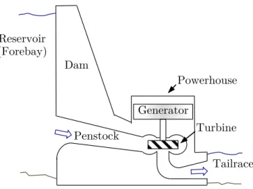
— As hydroelectricity is generated by the potential and kinetic energy of the water that drives the turbines of the system (Fig. 1.1), the total electricity production is a nonlin-ear function of the turbine discharges, the forebay elevation and the number of active generators (Fig. 1.2). Furthermore, generating units are also characterized by nonlin-ear efficiencies. All such nonlinnonlin-earities add complexity to the planning and operation of hydropower systems. Powerhouse Dam Penstock Reservoir (Forebay) Generator Turbine Tailrace

Figure 1.1 Schematic of a hydroelectric powerhouse. The stored water in the forebay flows through the penstock and propels the generating units of the system. The poten-tial energy of the water is proportional to the net water head, which is the difference between the forebay elevation and the tailrace elevation, minus the energy losses. — Due to the water storage capacity in hydropower systems, operating decisions are

cou-pled in time. Immediate decisions such as water discharges determine the water levels, which impact the future operating cost of the system. Thus, maintenance activities can be postponed, anticipated or expedited to maximize the electricity production, ac-cording to the current and expected stored water levels in the system. For example,

maintenance outages can be postponed when the water level is high, to reduce water spills with no economic benefit for the system.

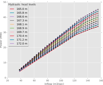
Hydraulic head levels!

Figure 1.2 Hydroelectricity production function of a generating unit in a powerhouse. The hydraulic water head level and the water discharge have a nonlinear effect on the hydroelectricity production.

— In cascade systems, decisions are spatially interdependent: water spills and turbine discharges can feed downstream reservoirs (Fig. 1.3).

u_g Upstream

inflows

vg

v_i

u_i

s_i Li Lateral inflows Plant outflows

Figure 1.3 Mass balance in a reservoir. Reservoir i is fed by water discharges v and water spills u from upstream reservoirs g. Reservoir i is also fed by lateral inflows F from tributary rivers or snow-melt. Adapted from Oliveira et al. (2002).

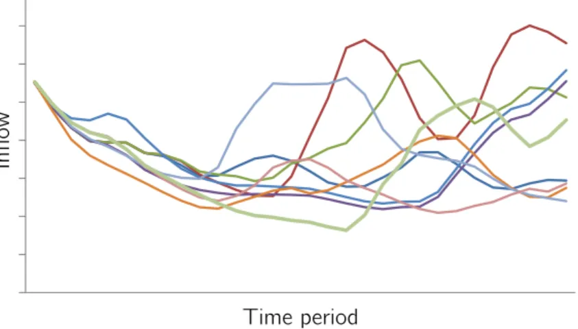
— Reservoirs are fed by tributary rivers, snow-melt and rainfall, which can exhibit large variability and are difficult to predict (Fig. 1.4). Therefore, maintenance scheduling in hydroelectric systems must account for the uncertainty in the hydropower operation.

Inflow

!

Time period!

Figure 1.4 Time series of 11 forecasted water inflow scenarios

1.3 Purpose of this study

In this dissertation, we address the Stochastic Hydropower Generator Maintenance Schedul-ing Problem (SGMSP), i.e., the maintenance schedulSchedul-ing of generatSchedul-ing units in hydropower systems, taking into account the nonlinearity of the electricity production, the uncertainty of the water inflows and the system interdependencies in space and time (Fig. 1.5). This problem can be stated as:

Given a list of maintenance activities to be completed within a specified planning horizon, find a maintenance schedule that maximizes the economic benefits of the electricity production, while considering the time windows, cost and duration of the maintenance activities, as well as maintenance constraints and essential characteristics of the hydropower operation.

This problem is motivated by a real case in Rio Tinto Aluminium, a multinational company that owns six powerhouses in Québec, with a total average generation of 2080 MW for its aluminium smelting operations. Through collaboration between two departments of the company, maintenance schedules are built manually, which can lead to delays and suboptimal schedules.

We apply mixed-integer programming techniques to obtain optimal solutions to this problem, using piece-wise linear approximations of the nonlinear hydroelectricity production. Due to the complicating aspects of the hydropower operation within maintenance scheduling, the

5

How to use a decomposition approach to efficently produce maintenance schedules that minimize the maintenance and operation costs in hydropower sytems?

Jesus Rodriguez, Miguel Anjos, Charles Audet and Pascal Côté

Hydropower provides 97% of the renewable electricity in Canada and 46% in the USA.

Maintenance outages

•  Extends lifetime of equipment •  Prevents costly breakdowns Maintenance of generators Time Uncertain Inflows Nonlinear power functions

Temporal and spatial interdependencies

Equation

Pt= f (Qt, ht, ⌦t)

Figure 1.5 Schematic of generator maintenance scheduling in hydropower systems. Mainte-nance schedules impact the hydropower operation, which is also affected by uncertain water inflows, nonlinearities in the electricity production and system interdependencies.

resulting model is hard to solve for real instances of the problem. Therefore, there is a need to tighten our model and to apply Benders decomposition with parallelization and acceleration techniques to solve the SGMSP with a large number of inflow scenarios.

This work comprises the following objectives:

1. To develop a tightened mixed-integer programming formulation for the generator main-tenance scheduling problem, considering the time windows of mainmain-tenance activities and the nonlinearities of the hydropower production function.

2. To implement a Benders decomposition method for the SGMSP with uncertain water inflows.

3. To accelerate the Benders decomposition method for the SGMSP by means of paral-lelization and acceleration techniques.

4. To propose extensions to the mathematical program for the SGMSP and to the solution approach.

1.4 Main contributions

We propose the first mixed-integer programming model for maintenance scheduling of gen-erating units in hydropower systems, considering the time windows of maintenance activities and the nonlinear effect of turbine discharges, hydraulic head and number of active generators on the electricity production. Moreover, we extend this formulation as a two-stage stochastic program, to represent the uncertainty of the water inflows in the hydropower operation.

We develop a compact formulation for this problem (in the sense of Williams (2013)) by ex-cluding unnecessary elements from the model. Because the generator maintenance schedul-ing problem is hard to solve even in the deterministic case, we tighten our model through valid inequalities, extended formulation and a set reduction method based on time windows information. Using statistical methods and computational experiments, we select the best combination of such tightening techniques based on instances adapted from a real hydropower system.

For solving the SGMSP with a large number of inflow scenarios, we implement a parallelized Benders decomposition method with seven acceleration techniques, and we show that a com-bination of five of these techniques achieves a fourfold speedup of the decomposition method applied to this problem. Due to a large number of potential configurations of the proposed acceleration techniques, we apply a sequential experimental design methodology to select the combination of such techniques with the best performance on the SGMSP.

We discuss extensions to our formulation for the SGMSP by including decisions on the duration of the maintenance activities and incorporating diverse maintenance constraints, such as available resources, energy reserves and precedence of activities. Finally, we show that an alternative decomposition approach, with a reduced master problem, can be applied to the SGMSP.

1.5 Plan of the dissertation

In Chapter 2, we introduce basic concepts of mixed-integer programming, Benders decompo-sition and maintenance scheduling, and we discuss related works. In Chapter 3 we describe the methodology of this study, and we highlight the connections between the subsequent chapters and the research objectives. Chapter 4 develops a tightened mixed-integer program-ming formulation for the deterministic generator maintenance scheduling problem. Chapter 5 extends this formulation as a two-stage stochastic program and develops a parallelized Ben-ders decomposition method with acceleration techniques for its solution. In Chapter 6 we present an alternative decomposition strategy for his problem and we enhance the proposed mixed-integer formulation by considering additional maintenance scheduling decisions and requirements. A synthesis of the work, along with a discussion of the limitations and future research is presented in Chapter 7. Chapter 8 presents the main conclusions.

CHAPTER 2 LITERATURE REVIEW

2.1 Basic concepts of mixed-integer linear programming

Many real-life decision-making problems consist in selecting, with respect to a list of quan-tifiable criteria, the best solution among a set of alternatives. In general, these problems can be specified as mathematical optimization problems (OP) of the form

optimize

x f (x), x∈ X (OP)

where x is the vector of unknowns that represents the alternatives of the problem, X is the set of feasible solutions, and f (x) is the function that measures the objective (or objectives when f (x) = (f₁(x), . . . , fk(x))) to be maximized or minimized, depending on the specific

problem. Typical objectives in optimization problems are profit, cost, distance, travelling time, emissions and social welfare, among many others. In single-objective problems, when f (x) is a linear function and the variables x are continuous with a feasible set X defined by linear inequalities, the optimization problem (OP) can be formulated as a linear program (LP) maximize x c |_x subject to: Ax_{≤ b,} (LP) l _{≤ x ≤ u,}

where A _{∈ R}n×m _{is the constraint matrix, b ∈ R}m _{is the vector of right-hand side terms of}

the constraints, c _{∈ R}n _{is the vector of the objective function coefficients, and u, l∈ R}n _are

the vectors of lower bounds and upper bounds, respectively, of the decision variables x_{∈ R}n_.

Linear programs have great applicability, not only for their suitability to represent a wide variety of real problems but also because of the availability of methods for their efficient solution (Dantzig, 2002).

Due to the convexity of the polyhedron P = _{{x ∈ R}n _{: Ax ≤ b; l ≤ x ≤ u} that describes}

the feasible set of LP and also because of the proportionality and additivity of the objective function c|_{x, if the feasible set P is not empty, an optimal solution to LP can always be found}

in one of its extreme points (Fig. 2.1). However, when some variables in x are restricted to integer values, i.e. in mixed-integer linear programs (MILPs), the extreme points of the linear relaxation solution defined by P may violate the integrality constraints (Fig. 2.2). For this

reason, when solving integer linear programs, removing fractional solutions and intelligently exploring the set of integer solutions are typical approaches (Nemhauser and Wolsey, 1988).

Feasible region a

b

Constraint 2 Optimal solution

to the linear program

0 1 2 3 0 1 2

x

x

Constraint 1 _{Objective function} isolines

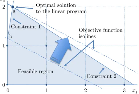
Figure 2.1 Graphical solution to a linear program with two constraints and two nonnegative variables, x₁ and x₂. The shadowed region represents the feasible set defined by constraints 1 and 2, and the variables’ nonnegativity constraints. The big arrow indicates the direction of improvement of the objective function (represented by the dashed isolines). The extreme point b is feasible but not optimal. The optimal solution to the linear program is given by a, which is the last feasible point reached by the objective function in the direction of improvement.

In general, strong formulations lead to LP relaxation solutions with a better approximation of the MILP solution. For example, in Fig. 2.2 a linear program with a feasible region whose extreme points are integer (represented by the shadowed area) has an integer optimal solution (3, 0), which is also an optimal integer solution for the original MILP. This smallest convex set that contains all integer feasible solutions is referred to as the convex hull.

2.1.1 General exact solution methods for mixed-integer linear programs

Because in some MILPs an exponential number of constraints would be necessary for de-scribing the convex hull, in practice only some constraints (or cuts) are included for refining the approximation of the integer feasible set (Nemhauser and Wolsey, 1988). Such cuts can be included a priori into the model, or they can be iteratively generated through a cutting plane algorithm (Wolsey, 1998).

Convex hull

c

x

x

a

Figure 2.2 Graphical solution to the problem in Fig. 2.1 with integer variables. Since the solution to the linear program is fractional (point a), the objective function must reduce its value until reaching an optimal integer feasible solution, which occurs at the point c. Notice that the closest integer points to the fractional solution a are either infeasible or suboptimal.

.

integer programs, in general, this approach is impractical when more than a few dozen integer variables are involved, due to the combinatorial explosion of the search space (Wolsey, 1998). A more efficient strategy implicitly enumerates the solutions while avoiding the exploration of sections of the feasible region that are unlikely to contain a better solution than the incumbent, i.e., the current best integer solution. Such a strategy is the basic idea of the LP-based branch and bound method, which using an enumeration tree, systematically computes bounds based on LP relaxations and splits the search space into disjoint sets that remove fractional values of the variables, while preserving all the integer solutions of the original problem (Land and Doig, 1960).

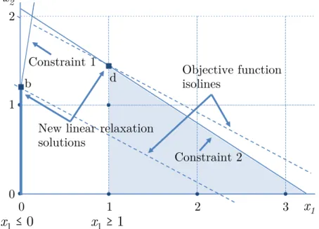
For example, in the linear program of Fig. 2.1, at the root node of the tree the solution a has a fractional value for x₁. A branch and bound algorithm then can branch on this variable to create two child nodes: one with the constraint x_{1 ≤ 0, and one with x1 ≥ 1, which remove} fractional values of x₁ and partition the feasible region as shown in Fig. 2.3. In active nodes with fractional solutions, the branching procedure continues, except when they are infeasible or when they are unpromising. For each parent node, the best LP relaxation value of its child nodes defines an upper bound. Indeed, any integer solution in either of its descendant nodes cannot be better than their LP relaxation value. Furthermore, any integer solution better than the incumbent defines a new lower bound, which is used to cut-off sections of the tree:

nodes with an LP relaxation dominated by the lower bound are fathomed (or excluded from further exploration). When the upper bound and the lower bound converge, the optimality of the incumbent solution is proven.

In practice, the execution of a branch and bound method can be time-consuming due to the slow progress of the bounds and the exponential increase of the tree size (Klotz and Newman, 2013). Cutting planes can be included at different steps of the branch and bound process, to speed up the solution by tightening up the formulation gradually. This solution approach, referred to as branch and cut, in combination with preprocessing, heuristics and parallel computing is an essential ingredient of state-of-the-art mixed-integer programming solvers (Ralphs et al., 2018; Bixby et al., 1999; Bixby and Rothberg, 2007).

Objective function isolines d b Constraint 1 Constraint 2 0 1 2 3 0 1 2

x

x

x

1

x

0

New linear relaxation solutions

Figure 2.3 Linear relaxation solution to an integer linear program after branching on the variable x₁.

Because in hard problems the computational time to reach an optimal solution with general methods can be prohibitive, suboptimal solutions may be acceptable in practice, based on their optimality gap. In absolute or relative terms, the optimality gap is defined as the difference between the incumbent solution and the best bound of the relaxation.

2.1.2 Decomposition methods for mixed-integer programs

Large mathematical programs typically involve interacting subproblems linked by a few con-straints or variables (Lasdon, 1970). In many cases, decomposition methods can exploit the

mathematical structure associated with this class of problems referred to as block angular, by splitting the original model into subsystems that are solved iteratively. Other structures such as bordered angular, block triangular and staircase are also characteristic of large systems (Bradley et al., 1977).

In primal block angular structures the subsystems interact only through a group of linking constraints. Such constraints usually represent global conditions of the problem, such as mass balance, shared resources or total demand to be satisfied. By relaxing the linking constraints, the block angular linear program

maximize x,y c | 1x1 + c|2x2. . . + c|pxp subject to: B₁x₁+ B₂x₂. . . + Bpxp ≤ b0 (Linking constraints) A₁x_{1 ≤ b1} A₂x_{2 ≤ b2} . .. .._. Apxp ≤ bp

splits into p independent subproblems

maximize x c | kxk subject to: Akxk ≤ bk, for k = 1, . . . , p.

Similarly, subsystems can be coupled by variables that usually represent decisions made in previous stages or in higher levels of the system. Such complicating variables can be subject to integrality requirements that destroy the convexity of the problem. As an example, in facility location problems, decisions on deliveries to customers are coupled across demand scenarios by strategic decisions on the capacity and location of the network’s facilities.

A linear program maximize c|₁x₁ + c|₂x₂ . . . + c| pxp + h|y subject to: A₁x₁ + B₁y _{≤ b1} A₂x₂ + B₂y _{≤ b2} . .. .._. Apxp + Bpy ≤ bp

with subsystems linked only by complicating variables y has a dual block angular structure. By fixing the variables y = ¯y, this linear program breaks into p independent subproblems: for k = 1, . . . , p, maximize x c | kxk subject to: Akxk ≤ bk− Bky.¯

For block angular linear programs, the two most common decomposition approaches are Lagrangian methods and methods based on the delayed generation of columns or rows of the model matrix.

Lagrangian methods relax the complicating constraints and include their violations as penalty terms in the objective function. In an iterative procedure, Lagrangian methods solve the resulting subproblems and update the penalty parameters. Such penalty parameters are ap-proximations of the Lagrangian multipliers, which represent the prices of the shared resources or the marginal cost of the linking constraints. In problems with integer variables, Lagrangian methods are especially efficient when the underlying network structure of the subproblems can be exploited to obtain integer solutions (Ahuja et al., 1988). Some methods of this class are Lagrangian relaxation (Geoffrion, 2010), Lagrangian decomposition (Guignard and Kim, 1987) and augmented Lagrangian (Boland and Eberhard, 2015).

Another family of decomposition approaches comprises Dantzig-Wolfe decomposition (Dantzig and Wolfe, 1961) and Benders decomposition (Benders, 1962), which partition block angular mathematical programs based on the fact that a polyhedron can be described by the convex combination of its extreme solutions. Dantzig-Wolfe and Benders decomposition are duals of each other (Lasdon, 1970). Whereas Benders decomposition is suitable for dual block angular structures, Dantzig-Wolfe decomposition can be applied to primal block angular linear

pro-grams. Dantzig-Wolfe (respectively, Benders) decomposition creates a master problem where the subproblems are represented by the primal (resp. dual) contribution of their extreme solutions to the original problem. Because the set of extreme solutions of the subproblems is potentially large, the decomposition algorithm sequentially includes, as needed, the columns (resp. rows) of the master problem corresponding to the contribution of the current extreme solution (Dantzig and Wolfe, 1961; Benders, 1962). To compute the extreme solutions of the subproblems and their marginal contribution, at each iteration the decomposition algorithm fixes in each subproblem the dual (resp. primal) variables of the master problem. When the master program is integer, Dantzig-Wolfe (resp. Benders) decomposition can be embedded in a branch-and-bound method, to generate columns (resp. rows) in the nodes of the tree, when necessary (Barnhart et al., 1998; Fortz and Poss, 2009; Desaulniers et al., 1998, 2006). Next, we give an overview of Benders decomposition, which is the solution approach applied in Chapter 5.

2.1.3 Benders decomposition

For the derivation of the Benders decomposition method (Benders, 1962), consider the math-ematical program maximize x,y c |_{x + f (y)} subject to: Ax + F (y) _{≤ b,} (P) x_{≥ 0,} y_{∈ S,}

where y is a vector of variables with a nonconvex feasible set S that makes the whole problem hard to solve. F (y) and f (y) are m-component and scalar functions, respectively, and x, c, b, A are as previously defined (see LP in Section 2.1). After fixing the complicating variables y = ¯y, the resulting subproblem

maximize x c |_{x + f (¯y)} subject to: Ax_{≤ b − F (¯y),} (SP) x_{≥ 0,}

is convex and thus much easier to solve. For simplicity of exposition we assume that for any y _{∈ S, the subproblem is feasible. By strong duality, the subproblem and its dual problem,} with variables π, have the same optimal value, i.e.,

Q(y) = maximize x {c |_{x : Ax≤ b − F (y) ; x ≥ 0},} = minimize π {[b − F (y)] |_{π : A}|_{π ≥ c ; π ≥ 0}.}

Furthermore, as the polyhedron A|_{u ≥ c , u ≥ 0 can be described by its set P of extreme}

solutions, Q(y) = minimize p∈P {[b − F (y)] |_πp }, = maximize zSP n zSP _{∈ R : z}SP _{≤ [b − F (y)]}|πp, _{∀ p ∈ P}o,

where the auxiliary variable zSP _{indicates the minimum value of the dual problem. With}

this reformulation of the subproblem SP, the original problem P can be rewritten as maximize

zSP_,y z

SP _{+ f (y)}

subject to: zSP _{≤ [b − F (y)]}|πp, _{∀ p ∈ P,} y_{∈ S,}

(MP)

which is the master problem (MP) of the Benders decomposition method. The role of con-straints

zSP _{≤ [b − F (y)]}|πp, _{∀ p ∈ P,} (2.1) referred to as optimality cuts, is to remove suboptimal solutions on the space of y, based on the extreme dual solutions of the subproblem. Due to the potentially large set of extreme solutions_{P, the Benders decomposition method relaxes the set of optimality cuts (2.1), and} sequentially includes violated cuts corresponding to new master problem solutions. Further-more, in problems where a master problem solution can produce infeasible subproblems, feasibility cuts can be sequentially included, using the extreme rays of the dual subproblem. At each iteration, the upper bound is the solution value of the relaxed master problem and the lower bound is the subproblem optimal value. When the bounds converge, the opti-mality of the solution is proved. The Benders decomposition method can also be applied to mathematical programs with multiple subproblems, by including cuts from aggregated or disaggregated subproblem solutions (Birge and Louveaux, 1988).

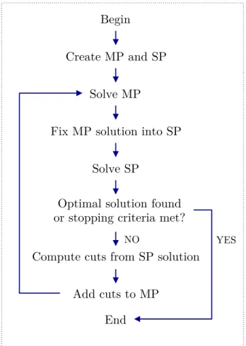
candidate solution ¯y, solves the subproblems with the fixed candidate solution y = ¯y, verifies the optimality of the solution and checks the stopping criteria, such as computation time and number of iterations. If the solution is not optimal and the stopping criteria are not met, optimality and feasibility cuts are computed and included into the master problem, and the process is repeated (see Fig. 2.4).

Create MP and SP

Solve MP

Fix MP solution into SP

Optimal solution found or stopping criteria met?

Compute cuts from SP solution Begin

End Solve SP

Add cuts to MP

NO YES

Figure 2.4 Flow diagram of the Benders decomposition method

Although Benders decomposition can, in principle, reduce the computational time by break-ing a hard problem into easy-to-solve subproblems, in practice its straightforward imple-mentation can yield poor convergence and time-consuming iterations (Rahmaniani et al., 2017; Magnanti and Wong, 1981). However, the Benders algorithm can be accelerated by adequately answering the following questions:

— What is an ideal formulation for Benders decomposition? Magnanti and Wong (1981) showed that, among multiple equivalent formulations of a mixed-integer pro-gram, the tightest formulation generates stronger Benders cuts and requires fewer iter-ations to converge. Therefore, valid inequalities and Benders cuts derived from solutions

to the LP relaxation of the master problem can speed up the solution (McDaniel and Devine, 1977; Cordeau et al., 2006).

— Which variables and constraints should be included in the master problem

and the subproblems? In non-trivial mixed-integer programs, there can be multiple

ways of partitioning the problem and of including auxiliary variables and constraints that help to approximate the original problem into the master problem and the sub-problems (Crainic et al., 2016; Gendron et al., 2016). The definition of the master problem and the subproblems is indeed a critical decision because it can determine the solution approach. For example, some problem partitionings can render integer subproblems or feasibility subproblems, which require special solution techniques and affect the type of cuts that can be generated (Hooker and Ottosson, 2003; Gendron et al., 2016).

— How to efficiently obtain solutions? Depending on the type of subproblem, special solution methods can be applied, such as network flow algorithms for network design problems (Magnanti and Wong, 1981), constraint programming for scheduling problems (Hooker and Ottosson, 2003) or Dantzig-Wolfe decomposition for crew pairing (Cordeau et al., 2001). Furthermore, when dealing with many subproblems, its parallel solution can significantly reduce the computational times. Similarly, multiple alternatives can be considered for the master problem solution, including heuristics and branch and cut (Laporte and Louveaux, 1993; Botton et al., 2013; Fortz and Poss, 2009; Fischetti et al., 2016a; Leitner et al., 2018).

— In the case of multiple subproblem solutions, which of them should be chosen

for generating cuts? In subproblems prone to multiple dual optimal solutions, such

as in network flow problems, each solution can generate a cut of different strength. Therefore, the convergence of the Benders algorithm can be accelerated by choosing a solution that generates the strongest cut (Magnanti and Wong, 1981). However, as the Magnanti and Wong (1981) approach for finding the strongest cut is computationally intensive, approximate methods have been developed for generating non-dominated cuts (Santoso et al., 2005; Papadakos, 2008; Cordeau et al., 2018).

— What type of cuts should be generated? When the subproblems are linear pro-grams, optimality and feasibility Benders cuts can be generated from the extreme points and extreme rays of the dual solutions (Lasdon, 1970). In the case of integer subprob-lems, lower bounding functionals (Laporte and Louveaux, 1993; Carøe and Tind, 1998) or through a logic-based Benders method (Hooker and Ottosson, 2003). Recently, An-gulo et al. (2016); Ljubić et al. (2017) and Álvarez-Miranda et al. (2017) showed that meaningful dual solutions of the LP-relaxation can be exploited in this context as well

for tightening the bounds of the master problem, before applying lower bounding func-tionals. For feasibility subproblems with binary variables, combinatorial cuts can be applied (Codato and Fischetti, 2006).

— At each iteration, how many cuts should we generate? In the case of multi-ple subproblems, at each iteration a single cut can be generated by aggregating the solutions of all subproblems. Alternatively, multiple cuts can be included by splitting the subproblems into clusters and computing a cut for each cluster at each iteration (Birge and Louveaux, 1988; Trukhanov et al., 2010). Although the multi-cut approach can reduce the number of iterations of the Benders algorithm, the effect on the compu-tational time is problem-dependent due to the larger size of the master problem with multiple cuts (Birge and Louveaux, 2011).

— How to improve the convergence of the decomposition algorithm? In the Benders master problem, large step sizes in the master problem solution tend to produce oscillation and to slow down the convergence of the algorithm (Birge and Louveaux, 2011). Some stabilization approaches for Benders decomposition restrict the distance from the previous master problem solution (Santoso et al., 2005), penalize in the master problem the deviation from the previous solution (Ruszczyński and Świetanowski, 1997) or minimize the distance to a pre-defined core-point Fischetti et al. (2016a,b).

For a recent review on Benders decomposition see Rahmaniani et al. (2017), and for a survey on applications of Benders decomposition to network design problems see Costa (2005).

2.1.4 Stochastic programming

In many practical problems, decisions take place in multiple stages, with realizations of un-certain problem parameters at each stage. In these problems, decisions are made in response to the revealed information up to the current stage and to decisions made in previous stages. Therefore, optimal decisions cannot anticipate the future realizations of the problem pa-rameters. For example, in capacity planning of electrical transmission systems, investment decisions occur in the first stage, and in subsequent stages the operating decisions of the electrical network take place in response to the electricity demand.

Although linear programming models are deterministic in nature, their application to mul-tiple stage optimization problems under uncertainty is possible through approaches such as stochastic programming and robust optimization (Birge and Louveaux, 2011).

In stochastic linear programming, the problem uncertainty is represented by scenarios ξ₁, . . . , ξK with probabilities p1, . . . , pK, which define a finitely supported joint distribution of

the random problem parameters ξ. In a two-stage stochastic linear program, the first-stage problem (FSP) with decision variables y can be formulated as,

max y ∈ Y c |_{y + E} ξ[Q(y, ξ)] subject to: Ay_{≤ b,} (FSP) y_{≥ 0,}

where Eξ[Q(y, ξ)] is the expected optimal value of the second-stage problem (SSP)

Q(y, ξ) = max x ∈ X q(ξ) |_x subject to: T (ξ)y + W (ξ)x_{≤ h(ξ),} (SSP) x_{≥ 0,}

with decision variables x, and random parameters T, W, h, q which depend on the specific realization of ξ. In this problem, x are the recourse actions made once the scenario parameters ξ and the decisions y are observed. The matrix W is typically assumed fixed (Shapiro et al., 2009) to characterize more conveniently the feasible region of the problem. The deterministic equivalent of the two-stage stochastic program can be obtained by replacing in FSP the expected value Eξ[Q(y, ξ)] by the weighted sum of the second-stage problems SSP,

and including their corresponding constraints. The resulting mathematical program maximize p₁q(ξ)|₁x₁ + p₂q(ξ)|₂x₂ . . . + pKq(ξ)|KxK + c|y subject to: W x₁ + T (ξ)₁y _{≤ h(ξ)1} W x₂ + T (ξ)₂y _{≤ h(ξ)2} . .. .._. W xp + T (ξ)Ky ≤ h(ξ)K Ay _{≤ b}

has a dual block angular structure that can be exploited via Benders decomposition when the number of scenarios is large (see Secs. 2.1.3 and 2.1.2). When the second-stage problems are integer, logic-based Benders decomposition and integer L-shaped method can be applied (Hooker and Ottosson, 2003; Laporte and Louveaux, 1993). In problems with multi-stages,

common solution approaches are nested decomposition (Birge and Louveaux, 2011), pro-gressive hedging (Rockafellar and Wets, 1991) and an extension of Benders decomposition referred to as dual dynamic programming (Pereira and Pinto, 1991).

2.2 Generator maintenance scheduling in hydropower systems

Before a revision of the previous works on maintenance scheduling of generating units in hydropower systems, we briefly discuss the principal issues in hydropower optimization and generator maintenance scheduling.

2.2.1 Planning and operation of hydropower systems

Planning and operation of hydropower systems involve decisions in multiple levels and plan-ning horizons, ranging from several decades to a few minutes (Barros et al., 2003; Cordova et al., 2014). In the higher level, generation capacity expansion decisions are assessed ac-cording to the expected returns of the hydroelectricity production over several years, or even decades, considering the optimal operating decisions under uncertainty of water inflows and electricity demand (Gorenstin et al., 1993).

For hydropower operation, the long-term planning, which typically spans several months, computes marginal values of stored water and target levels of reservoirs based on forecasted seasonal hydrological conditions (Bezerra et al., 2017). The mid-term planning defines main-tenance outages and target levels of the reservoirs, based on updated forecast information over several weeks. Short-term planning concerns the weekly operational schedule, as well as the commitment and loading of generating units. Usually, hours ahead of real-time operation, the unit commitment and loading problem determines the schedule of units for generation and ancillary services, as well as the water discharges, considering technical characteristics such as ramping rates and startup/shutdown phases of generators (Borghetti et al., 2008; Siu et al., 2001). In sub-hourly time spans, real-time control determines turbine discharges based on detailed calculations of generation efficiencies, energy losses and stored water levels (Cor-dova et al., 2014). Although the uncertainty of the water inflows in planning and operation of hydropower systems can be naturally addressed through stochastic dynamic programming (Bertsekas, 1995), its application in multi-reservoir systems is limited by the curse of di-mensionality that results from the discretization of the stored water levels in each reservoir. Due to this challenge, a variety of alternative approaches have been applied to hydropower operation, such as dual dynamic programming (Pereira and Pinto, 1991), progressive hedging (Carpentier et al., 2013), joint chance-constrained programming (van Ackooij et al., 2014)

and affine decision rules (Gauvin et al., 2017), among others.

For modelling the nonlinear hydroelectricity production, a compromise between solution quality and computational burden must be accepted. Some of the approaches for modelling the nonlinearity of such function are piece-wise linear approximations (Borghetti et al., 2008; Conejo et al., 2002; Ge et al., 2014; Marchand et al., 2018), nonlinear functions (Arce, 2001) and splines (Séguin et al., 2016) .

2.2.2 Generator maintenance scheduling

As discussed in Chapter 1, maintenance planning and scheduling are decision-making prob-lems that consist in finding the best compromise between the opportunity costs and the expected benefits of maintenance activities. While maintenance planning defines the main necessary maintenance activities, resources and recommended times of execution, based on maintenance policies (Dekker, 1996), maintenance scheduling determines the sequence and specific times of execution of the maintenance activities within specified time windows, con-sidering the available maintenance resources and the impact of the maintenance outages on the operational costs (Budai et al., 2008).

Due to the stochastic nature of the deterioration process and the failures, and also because of the difficulties for predicting the impact of maintenance activities on the system condition and the operation cost, the expected benefits and costs of maintenance are challenging to assess (Dekker, 1996). However, as the time windows of maintenance activities are relatively short with respect to the life-cycle of the equipment, in maintenance scheduling it is customary to neglect the equipment deterioration (Froger et al., 2016). Therefore, in maintenance scheduling the relevant costs are the opportunity cost of lost production due to maintenance outages, and the maintenance costs of overtime and outsourcing (Yamayee, 1982). All of these costs are determined by the time and duration of the activities in the maintenance schedule.

In the electricity industry, maintenance scheduling of generating units involves additional considerations:

— As a reliable electricity supply requires an instantaneous balance between consuming loads and power injections, maintenance scheduling must consider the impact of main-tenance outages on the generation capacity of the system (Billinton and Allan, 1996). — Due to the variability and uncertainty of i) electricity prices, ii) electricity demand, and

iii) power generation from intermittent renewable energies, significant savings can be achieved by postponing, advancing or expediting the required maintenance activities.

— To accurately assess the impact of maintenance schedules, it is necessary to consider the operating characteristics of the involved electricity-generating technologies (such as eolic, nuclear and hydropower), which can differ significantly.

For vertically integrated utilities, previous works have addressed the maintenance scheduling of generating units as optimization problems with objective functions related to reliability or operational cost (Froger et al., 2016). Multi-objective approaches for resolving the con-flicts between these two objectives have also been proposed (Moro and Ramos, 1999). To avoid the computational burden of probabilistic reliability measurements such as the loss of load expectation (Billinton and Allan, 1996), deterministic reliability indicators, such as generation reserve, have been commonly used in maintenance scheduling (Froger et al., 2016; Perez-Canto and Rubio-Romero, 2013).

In liberalized electricity markets, maintenance scheduling involves additional complications due to the interacting decisions of multiple self-interested market participants, such as private electricity producers, transmission companies and electricity retailers who want to maximize their profits. In such markets, an Independent System Operator (ISO) coordinates and controls the market activities to maximize the social welfare while guaranteeing the reliability of the electricity supply. Maintenance schedules proposed by the market participants must be revised and coordinated by the ISO through mechanisms such as contractual compensations (Dahal et al., 2015) or incentives (Conejo et al., 2005), to ensure the reliability of the system. Modelling all the aforementioned elements involved in generator maintenance scheduling leads to a hard problem for which typical solution approaches are heuristics, metaheuristics and mixed-integer programming with Benders decomposition (Froger et al., 2016).

2.2.3 Maintenance scheduling of generating units in hydropower systems

Despite the vast body of literature on maintenance scheduling in the electrical industry (see Froger et al., 2016, for a recent review), few works to date have addressed this problem in the context of hydroelectric systems. Furthermore, some works on maintenance scheduling that claim to have considered hydroelectric systems, have entirely neglected or oversimplified the most relevant aspects of the hydropower operation, such as the stored water effects, the uncertainty of the water inflows and the nonlinearities of the electricity production (Feng et al., 2011; Foong et al., 2008; Perez-Canto, 2008; Perez-Canto and Rubio-Romero, 2013; Chattopadhyay et al., 1995; Kuzle et al., 2010).

For long-term planning of preventive maintenance in hydropower systems, Jonsson (2015) used a dependency matrix for determining the sequence of activities in maintenance projects, and Welte et al. (2006) developed a Markov model of the equipment deterioration. Such

models did not represent the main operational aspects of the hydroelectricity production. Chattopadhyay et al. (1995) formulated a mixed-integer program for the coordinated main-tenance scheduling between interconnected utilities with different generation technologies. Their formulation did not include the operational characteristics of hydropower systems and assumed a fixed amount of available energy at each time period. For a deterministic genera-tor maintenance scheduling problem, Foong et al. (2008) developed an ant colony approach that uses simple heuristic rules for determining the turbine discharges, without regarding the effects of the nonlinear hydroelectricity production. Feng et al. (2011) represented the variability of the electricity generation with fuzzy variables but did not consider the relevant characteristics of the hydropower operation. Perez-Canto (2008), Perez-Canto and Rubio-Romero (2013) and Kuzle et al. (2010) presented mixed-integer programming formulations for maintenance scheduling, which assume constant power output in active generators and do not represent the operating characteristics of hydropower systems. For such formulations, Perez-Canto (2008) and Kuzle et al. (2010) applied Benders decomposition and Perez-Canto and Rubio-Romero (2013) proposed to search only for feasible solutions.

More realistic elements of hydroelectric systems have been considered in Régnier (2008), Guedes et al. (2015), Côté et al. (2015), Helseth et al. (2018) and Ge et al. (2018).

Régnier (2008) developed a heuristic method that uses an auxiliary function for assessing the effect of candidate schedules on the hydropower operation. Applying a black-box ap-proach, Côté et al. (2015) showed that important savings can be achieved by exploring the neighbourhood of an initial maintenance schedule, even if the new solution is not globally optimal. Guedes et al. (2015) implemented a genetic algorithm for a deterministic version of the generator maintenance scheduling problem, with continuous variables for represent-ing the startrepresent-ing times of maintenance activities within time window constraints. Although Guedes et al. (2015) represented the hydroelectricity production with an analytic function, their model neglects the nonlinear effect of the number of maintenance outages on the amount of produced electricity. More recently, Ge et al. (2018) developed a chance-constrained ap-proach for maintenance scheduling, with a piece-wise approximation of the hydroelectricity production, as in Ge et al. (2014), but without considering the nonlinear effect of the num-ber of active generators. Helseth et al. (2018) introduced a different approach for modelling the uncertainty in this problem, through a multi-stage stochastic optimization program with maintenance decisions in the first-stage and hydropower operation in multiple stages, solved by dual dynamic programming. Helseth et al. (2018) represented with a scenario tree the uncertainty of water inflows and demand, and approximated with piecewise segments the non-linearity of the hydroelectricity production with respect to turbine discharges.

How-ever, their formulation did not consider the nonlinear effect of reservoir levels and of the set of active generators, which substantially reduces the problem size but cannot realistically represent the nonlinearity of the hydroelectricity production function.

Concerning mixed-integer formulations of maintenance scheduling in the literature, we found three approaches:

1. Helseth et al. (2018) defined binary variables only for indicating the state of the gen-erators (i.e., active or in maintenance, as in Conejo et al. (2005)). Through algebraic constraints, this formulation explicitly controls the duration and continuity of mainte-nance activities across consecutive periods.

2. In Perez-Canto (2008) and Perez-Canto and Rubio-Romero (2013), two types of binary variables indicate the state of the generator and the beginning of maintenance activities. In such formulations, explicit constraints link the binary variables and control the duration and continuity of maintenance activities across consecutive periods.

3. Dahal et al. (2015) proposed a compact formulation, where only binary variables for indicating the beginning of maintenance activities are necessary and with the time windows controlled through index sets. Because in this approach the duration of main-tenance activities is controlled by index sets and not by algebraic constraints, its corre-sponding formulations are thinner and stronger than those correcorre-sponding to formulation approaches 1 and 2. However, this work did not address specific issues of maintenance scheduling in hydropower systems.

Our review of the literature on maintenance scheduling of generating units in hydropower systems, supports the following conclusions:

— Although the nonlinearity of the hydroelectricity production has been considered in recent works for obtaining globally optimal solutions to the problem (Helseth et al., 2018; Ge et al., 2018), the effect of stored water levels and number of active generators on the hydroelectricity production has not yet been appropriately addressed. Neglecting such elements can lead to poor estimates of the hydroelectricity production and to suboptimal solutions in practice.

— Considering the significant variability of the water inflows and their effect in the hy-dropower operation, alternative representations of the uncertainty, in addition to re-cently proposed chance-constrained (Ge et al., 2018) and scenario tree approaches (Helseth et al., 2018), should be explored to achieve an acceptable compromise be-tween solution quality and computational tractability.

— A more realistic representation of maintenance scheduling decisions is necessary, con-sidering other relevant objectives and constraints.

— Stronger formulations and alternative solution methods must be explored to find effi-ciently global optimal solutions to real instances of the problem, instead of local optimal solutions.

Considering these gaps in the literature, in the following section, we describe our approach for developing more realistic and efficient solutions to this problem.