UNIVERSITÉ DE MONTRÉAL
STOCHASTIC RICHELIEU RIVER FLOOD MODELING
MARYAM SAFARI
DÉPARTEMENT DES GÉNIES CIVIL, GÉOLOGIQUE ET DES MINES ÉCOLE POLYTECHNIQUE DE MONTRÉAL
MÉMOIRE PRÉSENTÉ EN VUE DE L’OBTENTION DU DIPLÔME DE MAÎTRISE ÈS SCIENCES APPLIQUÉES
(GÉNIE CIVIL) AOÛT 2018
ÉCOLE POLYTECHNIQUE DE MONTRÉAL
Ce mémoire intitulé :
STOCHASTIC RICHELIEU RIVER FLOOD MODELING
présenté par : SAFARI Maryam
en vue de l’obtention du diplôme de : Maîtrise ès science appliquée a été dûment accepté par le jury d’examen constitué de :
M. FUAMBA Musandji, Ph. D., président
M. MAHDI Tew-Fik, Ph. D., membre et directeur de recherche Mme HASSANZADEH Elmira, Ph. D., membre
ACKNOWLEDGEMENTS
I greatly appreciate Dr. Tew-Fik. MAHDI for his support, his patience, and his recommendations. I am proudly thankful of my valuable family that always support me in my life.
Special appreciations of my friends, my colleagues and Polytechnique Water engineering department’s students and professors that helped me during the Master program.
RÉSUMÉ
La modélisation hydrodynamique est un élément fondamental du génie hydraulique. Elle permet de créer des modèles de bassins versants et de rivières pour la prédiction des inondations. La simulation des phénomènes d'inondation est un sujet de plus en plus important dans le domaine de la recherche en hydraulique. Compte tenu des exigences d'évaluation spécifiques dans les plans d'ingénierie des risques d’inondation, la modélisation des inondations devient très importante dans le génie hydraulique. La délimitation probabiliste des zones inondables joue un rôle déterminant dans les plans d'ingénierie des risques. Cette tâche importante est réalisable à l'aide de la simulation post-inondation et de la détermination des limites de l'étendue des inondations avec leurs probabilités d'occurrence correspondantes dans les zones étudiées.
Au printemps 2011, les inondations de la rivière Richelieu, (Québec, Canada), ont fait l’objet d’une grande attention. Celle-ci a été concentrée dans les zones inondées binationales (à la frontière canado-américaine).
Dans la présente étude de cas, la rivière Richelieu a d'abord été modélisée avec un modèle unidimensionnel intégré au logiciel WMS (v.10.1) (Watershed Modeling System). Dans ce logiciel de modélisation, la rivière Richelieu a été définie par sa ligne médiane et ses sections transversales le long des 53 km sélectionnés pour l’étude. À l’aide de WMS, les étapes suivantes consistent à extraire les sections transversales à partir du modèle de terrain et à les affecter dans leur couche de couverture correspondante l'extraction des sections transversales. Ensuite, le plan détaillé de ce bassin versant et de cette rivière, avec des couvertures matérielles spécifiques, a été créé et a été transféré à HEC-RAS (v. 4.1).
Pour réduire les incertitudes des divers paramètres appliqués, il a été nécessaire de calibrer les coefficients de rugosité de la rivière Richelieu et des plaines inondables. Le premier essai de calibration a été effectué en utilisant l'option de calibration automatique du coefficient de Manning (rugosité) dans HEC-RAS. Les coefficients estimés par cet essai n'étaient pas dans une plage acceptable. Ce problème a été résolu en optant pour un autre logiciel de calibration automatique, PEST (v. 15). Puisque le fichier de sortie de HEC-RAS (un fichier binaire) n'était pas lisible par le logiciel PEST, le modèle hydrodynamique GSTARS (v. 3.0) a été choisi pour son utilisation des
fichiers textes. Sur la base des fichiers de sortie de GSTARS (v. 3.0) et des fichiers d’entrée de PEST, les coefficients de Manning ont été calibrés. Les conditions aux limites amont et aval ont été choisies pour maintenir la stabilité numérique du modèle. L'élévation de la surface de l'eau observée à la station de contrôle a servi de repère pour minimiser les différences entre les valeurs mesurées et simulées.
Avec les coefficients de Manning estimés pour la rivière et la zone inondée, et avec les conditions aux limites appliquées selon les informations enregistrées, la crue a été simulée dans HEC-RAS (v. 4.1). En retournant au logiciel WMS (v. 10.1), la délimitation probabiliste de la zone inondable a été obtenue. Cette délimitation se base sur la méthode de Monte Carlo et donne les pourcentages d'occurrence correspondants.
WMS (v.10.1) exécute le modèle stochastique en sélectionnant des variables d’entrée provenant d’une méthode probabiliste pour des durées d'exécution de simulation spécifiées. Les résultats de ce modèle unidimensionnel ont été comparés aux résultats du modèle bidimensionnel (SRH-2D) pour l'évaluation de l'efficacité et de la précision de chaque modèle utilisé. Les cartes des risques d'inondation de la rivière Richelieu, établies avec les deux modèles appliqués, pourraient permettre d'élucider les facteurs de risque d'inondation en termes hydrologiques, hydrauliques et de gestion. Cela peut aider à gérer de manière probabiliste les futures inondations et réduire les effets pertinents dans les plans de gestion du risque.
ABSTRACT
Hydrodynamic modeling including watershed, river and flood modeling is a fundamental part of hydraulic engineering. In this regard, simulation of flood phenomena is an increasingly important subject in hydraulic research domain. Considering specific evaluation requirements in flood risk engineering plans, flood modeling is becoming highly important based on hydrological method (rainfall-runoff) or hydraulic parameters in Hydraulic engineering.
Delineation of probabilistic flooded areas plays a specific role in risk engineering plans. This important is achievable with the help of post-flood simulation and determination of the flood extent borders with their corresponding occurrence probabilities in the studied areas.
Richelieu River flood in Quebec, Canada, occurred in the spring of 2011, was selected to be modeled in the present case study. Primarily, the Richelieu River was modeled with the aid of the one-dimensional Watershed Modeling System (WMS (v.10.1)). In this watershed modeling system, the Richelieu River was defined by its centerline and the cross sections along its 53 km selected length. Extracting the cross sections and assigning them in corresponding coverage layer in WMS were the next steps. Then, the detailed plan of this watershed and river, with specific material coverages, was created and was transferred to HEC-RAS (v.4.1).
For reducing the uncertainties of various applied parameters, calibration of the roughness factors of Richelieu River and flood plains were necessary. The first trial calibration was performed using the automatic roughness calibration option in HEC-RAS, but the estimated coefficients were not in an acceptable range. This issue was resolved by opting for another calibration software, PEST (v.15). Since the output file from HEC-RAS (a binary file) was not readable by PEST, the text input file was prepared using GSTARS (v.3.0). Based on the output files of GSTARS (v.3.0) and other input text files of PEST, the Manning coefficients were calibrated using the stable part of applied set of upstream and downstream boundary conditions. The observed water surface elevation at the control station was attained by minimizing the differences between the measured and simulated values.
Considering the estimated river and the flooded area Manning coefficients and the applied boundary conditions according to recorded information, the flood was simulated in HEC-RAS (v.4.1). Delineation of the probabilistic flooded area by referring to WMS (v.10.1) was considered. Based on the Monte Carlo method, WMS (v.10.1) delineates the probabilistic flooded areas with corresponding occurrence percentages. WMS (v.10.1) runs the stochastic model by selecting input variables in a probabilistic method in specified simulation run times. Furthermore, results of this one-dimensional model were compared with the results of two-dimensional model (SRH-2D) for the evaluation of efficiency and precision of each applied model. Based on this comparison, computational process in two-dimensional model is longer and more complicated versus brief one-dimensional one. Although, two-one-dimensional models are more accurate than one-one-dimensional method, but according to existing modellers, delineation of probabilistic flooded areas based on Monte Carlo method is achievable via dimensional method. Then in this case, WMS as a one-dimensional modeling system, can accomplish this research goals. Flood risk maps of the Richelieu River with the two applied models could elucidate the flood risk factors in hydrological, hydraulic, and managerial terms. This can help managing probabilistic future floods and decrease the relevant effects in risk plans.
TABLE OF CONTENTS
ACKNOWLEDGEMENTS ... III RÉSUMÉ ... IV ABSTRACT ... VI TABLE OF CONTENTS ... VIII LIST OF TABLES ...XII LIST OF FIGURES ... XIII LIST OF SYMBOLS AND ABBREVIATIONS... XVI
CHAPTER 1 INTRODUCTION ... 1
CHAPTER 2 LITERATUR REVIEW ... 2
2.1 Literature review ... 2
2.2 Project Objectives ... 8
2.3 Project hypothesis ... 8
2.4 Hydrodynamic modeling approach ... 8
WMS (v10.1) presentation ... 9
What's new in WMS (v10.1) ... 10
Introduction to HEC-RAS (v4.0.1) ... 10
CHAPTER 3 DATA GATHERING ... 14
3.1 The case study ... 14
3.2 Background case study ... 15
3.3 Data gathering and preparation ... 19
Geo data base ... 19
Soil cover ... 19
Topographical data ... 20
Satellite image ... 20
Other applied maps ... 21
Flood recorded information ... 21
Editing basic geographical information (DEM, TIN) ... 24
Rebuilding DEM ... 24
3.4 One-dimensional model characterization ... 25
Defining project in WMS ... 25
Specifying river banks ... 26
Creating cross sections ... 26
Defining centerline ... 27
Material coverage ... 28
Roughness coefficient ... 29
CHAPTER 4 METHODOLOGY ... 33
CHAPTER 5 NUMERICAL MODELING ... 35
5.1 Model calibration ... 35
5.2 GSTARS (v.3.0) ... 36
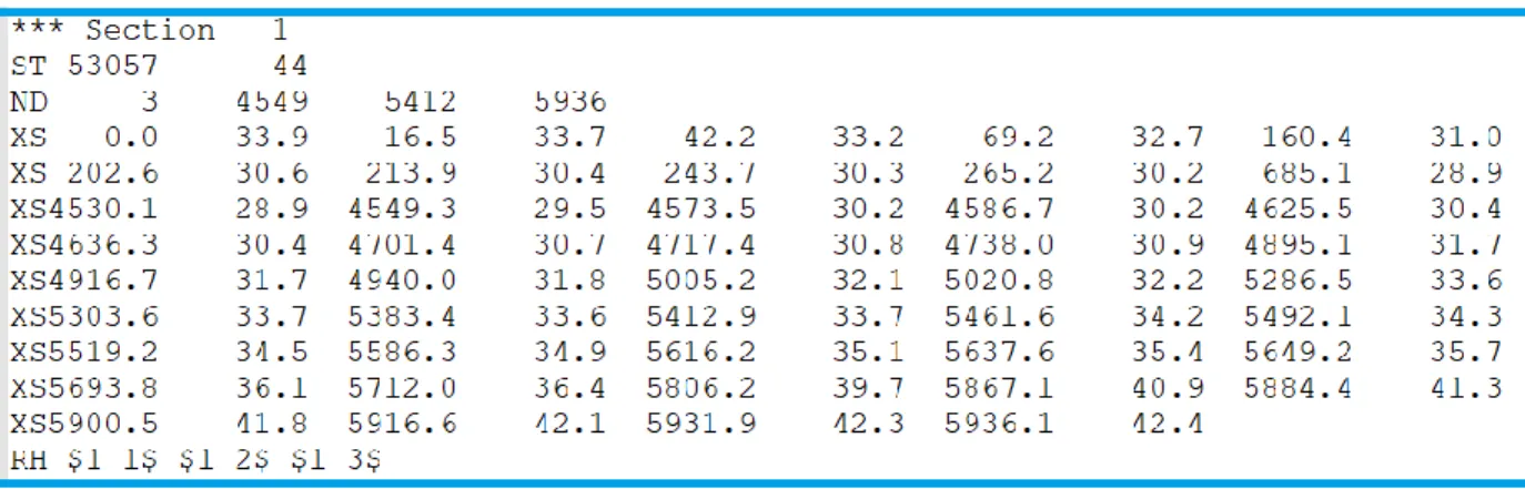
Preparing GSTARS input file ... 36
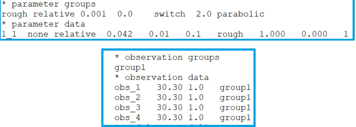
5.3 Parameters estimation: PEST ... 37
PEST utilities ... 40
PEST template file ... 40
PEST instruction file ... 41
PEST control file ... 41
Running PEST ... 43
5.4 Flood Simulation ... 45
HEC-RAS ... 45
Courant number ... 45
Performing the unsteady flow analysis ... 46
5.5 Probabilistic flooded area delineation ... 47
Monte Carlo method ... 47
Flood plain delineation and mapping criteria’s ... 47
Running stochastic model ... 48
CHAPTER 6 RESULTS AND ANALYSIS ... 49
6.1 HEC-RAS calibration result ... 49
6.2 PEST results ... 50
Calibration evaluation ... 52
6.3 HEC-RAS results ... 52
6.4 WMS results ... 57
Flood delineation ... 57
Probabilistic flooded area ... 60
WMS results analysis ... 73
Simulated flooded area in SRH-2D ... 76 CHAPTER 7 DISCUSSION AND RECOMENDATION ... 79 BIBLIOGRAPHY ... 82
LIST OF TABLES
Table 2-1: Provided contents by module in project explorer (WMS manual, AQUAVEO) ... 10
Table 3-1: Flood recorded data in three hydrometric stations (Morrissette Pare ,2014) ... 22
Table 3-2: Project details ... 25
Table 3-3: Roughness coefficients of Richelieu River and flood plains ... 30
Table 3-4: Suggested Manning coefficients (Chow, 1959) ... 31
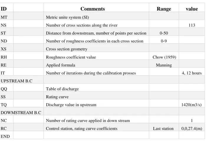
Table 5-1: GSTARS input data ... 37
Table 5-2: Selected flood duration for calibration ... 37
Table 5-3: Unsteady flow analysis options ... 46
Table 6-1: Calibrated Manning coefficients by HEC-RAS ... 49
Table 6-2: Calibrated Manning coefficient using PEST ... 50
Table 6-3: Flood depth frequencies information ... 71
Table 6-4: Calibrated manning in SRH-2D model (Morrissette Pare, 2014) ... 75
Table 6-5: Simulated water surface elevations and discharge using SRH-2D (Morrissette Pare ,2014) ... 75
LIST OF FIGURES
Figure 3.1: Location of Champlain Lake and Richelieu River, Quebec (Google earth, 2018) ... 16
Figure 3.2: Location of hydrometric stations in the studied area (world topo map, 2018) ... 17
Figure 3.3: Satellite images (NASA,2011): a (before flood), b (during flood), c (infrared image during flood) ... 18
Figure 3.4: Richelieu River material cover map (Morrissette Pare, 2014) ... 20
Figure 3.5: The corrected stage hydrograph applied as upstream boundary condition ... 23
Figure 3.6: Adjusted rating curve applied as downstream boundary condition ... 23
Figure 3.7: Background map with mild contour lines and stream networks, Richelieu watershed, 2017 ... 25
Figure 3.8: Right and left Richelieu River banks in studied area ... 26
Figure 3.9: One-dimensional Schematic Richelieu River in HEC-RAS ... 28
Figure 3.10: Sample cross section of Richelieu River (station:16465.5) assigned to WMS ... 32
Figure 4.1: Methodology diagram ... 34
Figure 5.1: PEST template file for sample station ... 40
Figure 5.2: PEST instruction file ... 41
Figure 5.3: PEST control file (variable presentation) ... 42
Figure 5.4: PEST control file (parameter group) ... 42
Figure 5.5: PEST control file (observation group) ... 43
Figure 5.6: Control file (command line) ... 43
Figure 5.7: Control file (Batch file) ... 44
Figure 5.8: PEST diagram ... 44
Figure 6.2: Initial Manning values versus estimated values using PEST ... 51
Figure 6.3: Estimated water surface elevation ... 51
Figure 6.4: Simulated water surface elevation in Control station (HEC-RAS) ... 54
Figure 6.5: Maximum simulated water surface elevation profile in HEC-RAS ... 54
Figure 6.6: Simulated water surface curve in the selected (third) cross section ... 55
Figure 6.7: Simulated water surface curve in the selected (last) cross section ... 55
Figure 6.8: Simulated water surface elevations histogram (113 cross sections) using HEC-RAS 56 Figure 6.9: Simulated water surface using HEC-RAS (plan view of Richelieu River) ... 57
Figure 6.10: Flood depth map of Richelieu River with background world imagery map (WMS on-line map, 2018) ... 58
Figure 6.11: Flood depth map from Rous Point to St. Paul with NASA image (2011) background ... 59
Figure 6.12: Flood depth map in two selected distance(a) and (b) with NASA image (2011) background ... 60
Figure 6.13:Probabilistic Richelieu flooded areas in WMS and NASA and word imagery. tif background images (2011) ... 62
Figure 6.14:Probabilistic flooded areas in Richelieu River (first part: 0-6.5 km of studied area) . 63 Figure 6.15: Probabilistic flooded areas in Richelieu River (second part: 6.5-14.5 km of studied area) ... 64
Figure 6.16: Probabilistic flooded areas in Richelieu River (third part: 14-20 km of studied area) ... 65
Figure 6.17: Probabilistic flooded areas in Richelieu River (fourth part: 20-25 km of studied area) ... 66
Figure 6.18: Probabilistic flooded areas in Richelieu River (fifth part: 25-30 km of studied area) ... 67 Figure 6.19: Probabilistic flooded areas in Richelieu River (sixth part: 30-40 km of studied area)
... 68 Figure 6.20: Probabilistic flooded areas in Richelieu River (seventh part: 40-45 km of studied area)
... 69 Figure 6.21: Probabilistic flooded areas in Richelieu River (seventh part: 45-53 km of studied area)
... 70 Figure 6.22: Flood depth frequencies of Richelieu river (WMS) ... 71 Figure 6.23: The frequencies of simulated water surface elevations in Richelieu river in composed interpolated nodes in the last time step ... 72 Figure 6.24: Simulated water surface Richelieu flood (a)and responding flooded area(b) (in purple colour and material cover map) using SRH-2D (Morrissette Pare, 2014) ... 76 Figure 6.25:Richelieu flooded areas (WMS, NASA, SRH-2D) ... 78
LIST OF SYMBOLS AND ABBREVIATIONS
BC Boundary condition DEM Digital elevation model
GSTARS Generalized Sediment Transport model for Alluvial River Simulation HEC-RAS Hydrologic Engineering center's River Analysis System
SMS Surface-water modeling system TIN Triangle irregular network WMS Watershed modeling system W.S. E Water surface elevation 1D One-dimensional model 2D Two-dimensional model 3D Three-dimensional model
CHAPTER 1
INTRODUCTION
Floods and flood risk management are recognized as hydrological-hydraulic challenges. In flood risk plans, comprehensive and effective approaches are essential, since this issue is strongly related to both environmental and human-related factors. Determinants of flood causes are categorized in three: meteorological, hydrological, and human (Ramkrishna and Pravin, 2014). Climatological factors consist of precipitation (rain or snowfall, snowmelt), storms and temperature fluctuation. Hydrological elements include soil moisture level, regional ground water level, natural surface infiltration, impervious cover, hydraulic elements of network channels and rivers (cross section, bed slope, and roughness coefficient of river bed and coastal area) (Ramkrishna and Pravin, 2014). Human-related factors, on their part, include urbanization, land use change, inadequate infrastructure in coastal areas, and insufficient flood control measures in hydrometric stations (Ramkrishna and Pravin, 2014).Therefore, flood risk management is a procedure concerning risk analysis, mitigation and risk control, preparedness, and respond in the case of natural disasters (Plate, 2002). Such disasters comprise storms and floods owing to natural and environmental hazards and human interference. For risk minimizing, decision makers consider the severities of the vulnerabilities and design and present protection plans to increase the safety level in flooded areas (Plate, 2002). Flood risk management has thus been defined as a functional framework to estimate and evaluate losses and vulnerabilities for construction and human life in probabilistic flooded areas (Plate, 2002).
Hydrodynamic modeling as an increasingly developing domain, applies various modelers (different hydraulic and hydrological oriented software), has a truly key role in hydraulic and hydrologic research field. Hydrodynamic modeling could be a useful representation of the phenomena based on real flow conditions, simulating watersheds, rivers and floods for assessment, reconstruction and forecasting (Plate, 2002). Modeling of phenomena by the aim of simulation of previously occurred phenomena and probabilistic future ones, is an approach that can help the researchers to assess, to evaluate, and to predict the phenomena occurrence with the accurate technical details.
CHAPTER 2
LITERATUR REVIEW
In this chapter with the aim of clarifying thesis subject, various points of view concerning flood, risk engineering, flood risk mitigation, flood modeling and importance of selecting modellers will be discussed. Also, the general technical aspects of applied software in simulation of Richelieu Flood in 2011, will be introduced. The frame works of main applied software: WMS (V10.1) and HEC-RAS (V 4.1) as two main software, are presented to justify the rationale basis of their selection.
2.1 Literature review
Flood risk management could be categorized in risk analysis, disaster mitigation, preparedness, and disaster response (Hansson, Danielsona & Ekenberga, 2008). Risk analysis involves determination and measurement of risk levels and estimation of relevant vulnerabilities. The second factor (disaster mitigation) defines disaster mitigation plans using technical and non-technical methods (Hansson, Danielsona & Ekenberga, 2008). The third element (preparedness) consists of disaster relief planning, early warning schemes, and evacuation plans. Disaster response involves emergency help and rescue considering in different flood protection systems. This factor is defined by the risk sensitivities of each case priorities for implementation of a desirable and comprehensive flood risk exposure system (Hansson and Danielsona & Ekenberga, 2008). To make risk plans, the effective set of parameters for evaluation of flood risk management are differentiated by the priorities and main concerns of their respective stakeholders (Plate, 2002). Furthermore, the affected nation’s economic strength plays a significant role in determining an appropriate plan (Plate, 2002). It is evident that developing countries suffer from lack of effective and sufficient institutional systems for the implementation of early warning technologies, prevention and minimization of flood side effects (Plate, 2002). Some of the determining parameters included in a decision model are crisis management criteria, warning system and education plan, insurance plan, reliable measurement systems and structural and non-structural defense (Plate, 2002). These factors can be helpful in a complete modeling bio-hazardous system implementation in order to being prepared for high-risk flood areas.
There are structural procedures to cope with floods including flood embankments, new flood channels (drain channels), watershed management, and detention reservoirs (Ramakrishna and Pravin, 2014). These methods could be applied according to the existing possibilities and the potential options. Non-structural methods include: the preparation of Probabilistic flood maps, forecasting and warning strategies, evacuation and relocation plans in dangerous areas, and flood insurance (Ramakrishna and Pravin, 2014). Planning ahead is another effective strategy, since populations in probabilistic flooded areas have increased dramatically in the last century due to urbanization and land use changes (Ramakrishna, Pravin S, 2014). Additionally, the clear majority of disaster losses is related to human decisions, because several possible existing actions are served coping with floods such as alertness strategies (Benson and Clay, 2004).
The estimation of resulted losses in flooded areas could be a key factor in making risk analysis plans. To be able to do this, an accurate estimation of involving elements is necessary. In risk flood management frameworks, losses may be categorized as direct and indirect, and tangible and intangible ones (Ramkrishna and Pravin S., 2014). Direct losses are defined due to direct contact with flood water, losses in buildings, infrastructures, and animals. Indirect losses are resulted indirectly from floods including transport disruptions and business losses (Ramkrishna and Pravin, 2014). Other relevant losses are tangible ones, which are related to things with monetary value as well. Intangible losses are associated by items that cannot be bought and sold. These losses involve vital items leading to increase of sickness or homelessness among populations (Ramkrishna and Pravin, 2014).
Another important factor in evaluation of flood issues is uncertainties in flood mappings. In making probabilistic flood maps, there are some inherent parameters which are associated with uncertainties including precipitations (frequency, duration, intention), measured stream flow (peak value, location, recorded duration) (Merwade, Olivera, Arabi, Edleman, 2008). Topographical uncertainties which are associated with applied maps with different accuracies are other sources of error in final modeling results (Merwade et al, 2008). The modeling parameters and techniques which are applied by different modeling software are considerable source of uncertainties (Merwade et al, 2008). Furthermore, the propagation of mentioned individual hesitation element and how they can cumulatively affect overall uncertainties in final flood maps are considerable.
Flood mappings are considered as specifying areas covering by water during inundations. To do this, some hydrological parameters like estimation of peak flow in corresponding duration and hydraulic elements such as water surface elevation are important parameters of creating one-dimensional models (Haberlandt and Radtke, 2014; Merwade et al, 2008). Involving hydrologic and hydraulic parameters are mainly investigated as following’s.
The design flow which can be obtained by corresponding flood frequency information, recorded data from nearby stations or regional flood record stations and hydrologic modeling based upon rainfall-runoff data (Haberlandt and Radtke, 2014; Merwade et al, 2008). Geometrical parameters include created cross sections, roughness coefficients and river and floodplains slopes. These mentioned parameters can significantly affect by hydraulic modeling analysis (Haberlandt and Radtke, 2014; Merwade et al, 2008). These parameters comprise of discharge values which are derived of corresponding hydrologic model and water surface elevations which are determined by hydraulic models and flood extents (Haberlandt and Radtke, 2014; Merwade et al, 2008).
Flood Frequency Analysis (FFA) has a great value to flood risk assessments and develop respective protection plans. There are two main approaches to determine flood frequency analysis. The first approach is classical or traditional approach which consist of long-term observational records of floods information (Hosking and Wallis, 1988; Haberlandt and Radtke, 2014). The second approach is simulating floods based upon hydrological and hydraulic elements.
Flood modelling is defined in two main steps. The first step introduces hydrologic models to estimate design flood hydrographs which requires several input variables include design rainfall based on durations, intensities and temporal patterns and determine respective losses. The last input variable group comprises base flow and flow routing parameters witch are associated with degree of uncertainties by impacts on final flood hydrographs parameters like magnitudes and forms (Rahman,Weinmann & Hoang, Laurenson & Nathan, 2002). The second step covers application of hydrological results: designed flood hydrographs as input parameters into hydraulic models to approximate probabilistic flooded zone (Rahman, et al, 2002). By considering how hydraulic analysis can be affected by mentioned uncertainties, some flood modelers smear the Monte Carlo simulation method to estimate flooded areas. Mathematically, this simulation method based on the joint probability approach by making random sampling (xi) (i: 1,…, n) (is uniformly
distributed over continuous rang (0,1)) on input variables and conducting many experiments on them according to their distribution F(xi) can evaluate the output (Y). The performance function can display the characteristics of these experiments (model output). Then statistical analysis of results let us have mean, variance, reliability, pdf (probability density function) and cdf (cumulative distribution function) (Siddall, 1983). In traditional rainfall-runoff modeling approaches, flood simulation encounters various restrictions due to lack of considering the stochastic nature of flood key elements in creating flood hydrographs (Charalambous, Rahman & Carroll, 2013). This alternative method (the Monte Carlo simulation) based on joint probability is employed to produce designed flood by using random variables instead of fixed ones (Charalambous, Rahman & Carroll, 2013). The Monte Carlo method with more flexibilities and more realistic estimations in numerous scenarios could provide greater results is replaced by traditional methods (Charalambous, Rahman & Carroll, 2013).
The effect of different design parameters on flood routing is another subject to investigate. Design parameters include watershed topography and geometry, river bathymetry and modeling approaches. Furthermore, by considering impacts of mentioned factors separately and overall, the delineation of floodplains could be more accurate (Cook and Merwade, 2009).
In Stroud’s Creek (case study), the effect of topographical changes on the river size and the modelling method was investigated (Cook and Merwade, 2009). Final results of flood simulation using HEC-RAS confirmed that in finer resolutions of topographic data tests, predicted inundation areas was decreased (Cook and Merwade, 2009). In addition, with the same number of two-dimensional inundation cells (FESWMS) in coarser topography dataset, further areas were generated in comparison with finer data (Cook and Merwade, 2009). In the same case study, the effect of geometric descriptions was assessed as well. Defined geometric descriptions include numbers and locations of cross sections and structural details in the one-dimensional model (HEC-RAS) in corresponding flooded areas. The sensitive analysis on geometric data showed that by increasing the number of cross sections the produced flooded areas were extended (Cook and Merwade, 2009).
Different types of hydrodynamic modeling include 1D, 2D and 3D are available to investigate flood modeling in terms of various-dimensional models. Although 1D method versions are
computationally effective, number drawbacks like simulation inability in lateral diffusion of the flood wave and subjectivity in discretization of topographical information as locational cross sections instead of continuous surface exist in theses models (Teng et al, 2017).One-dimensional methods represent flooded areas using created cross sections and solving the momentum and mass conservation laws by St-Venant equations (1D) between each two cross sections can estimate floodplain elements like water discharges and water elevations(Teng et al, 2017). Two-dimensional modelers by solving full shallow water equations of depth-averaged Navier-Stockes equations and considering x and y as two spatial directions and two-dimensional velocity (u,v) and water depth over space and time during each time step could accurately simulate timing and duration of desired inundation (Teng et al, 2017). By investigating the effect of modeling approach on flooded areas reported by (Cook, Merwade, 2009), the estimation of flow design could be still based on methods that have been developed from 20 years ago. One-dimensional modeling (1D) is still the standard practice in flood simulation and delineate flood maps. Cook and Merwade, 2009 confirmed that the selection of modeling approach (1D/2D) is still a challenging issue for delineation of accurate flooded areas. In cases with the limitation of topographical data, the1D modeling methods like HEC-RAS in comparison with 2D modelers like FESWMS-2HD could produce equally good results in flooding maps (Cook, Merwade, 2009).It should be noted that predicted inundation maps by 2D models can be more accurate due to fewer variations in hydrologic and hydraulic applied data, but some limitations such as time consuming and more computational process should be considered too (Cook, Merwade, 2009).
Three types of applied approaches in flood modeling: empirical, hydrodynamic, and simplified methods could have potential research subject attractions. The empirical methods are data-based methods combine measurements, surveys, and remote sensing methods (Baldassarre, Schumann, Bates, 2009). These methods are recognised as straightforward approaches to derive flood data using observational methods. The inability of prediction of future change, environmental and device-associated limitations, could be considerable as disadvantages of these methods (Teng, Jakeman, Vaze, Croke, Dutta & Kim, 2017).
Hydrodynamic methods are the most widely used tools to simulate detailed flood dynamics. They can be directly linked to hydrological models and river models to provide flood risk mapping,
flood forecasting and scenario analysis (Teng et al, 2017). These methods dissimilar to empirical methods, could be able to investigate impacts of changing determining factors like initial and boundary condition sets on final results, by possibilities of manipulating input data (Teng et al, 2017). There is no analytical solution for St-Venant equations, so numerical methods are applied to solve them. Neelz and Pender, 2009 have also pointed out strong differences in modelling results, especially for flood prediction using 1D river to 2D floodplain linkage, and for velocity predictions in urban areas. Despite active research in this field, rapid and accurate flood modelling at high spatial-temporal resolutions remains a significant challenge in hydrologic and hydraulic studies (Teng et al, 2017).
In determination of probabilistic flooded areas, river and watershed model calibrations recognized as fundamental factors. Reducing differences between measured and simulated data in acceptable range via calibration is an important part of every simulation method. In this regard, recognizing the most determined element(s) needs accurate numerical and experimental analysis. Automatic model calibration using PEST as an optimiser software in hydraulic domains has a great value. (Lavoie and Mahdi, 2017) applied PEST as an independent and relatively simple model and also as a powerful tool for the calibration of two-dimensional hydrodynamic models. In order to verify the precision of Manning coefficient(s) of rivers and sensitive analysis in steady and unsteady state flow, (Lepage, 2017) utilized PEST as well.
On conclusion, in this case study research, the probabilistic flooded areas of Richelieu River were determined by using WMS and HEC-RAS in one-dimensional type, which have not been investigated till now. Besides, the important hydraulic factor in this case study research was roughness coefficients in river bed and floodplains which automatically was calibrated by running PEST. Then based on calibrated roughness factors and boundary condition sets, the Richelieu flood was simulated using HEC-RAS. Finally, probabilistic flooded areas based on the Monte Carlo method in WMS, were delineated according to their appropriate occurrence percentages. Results of WMS (one-dimensional) and SMS (Surface-water Modeling System) as an interface of SRH-2D, two-dimensional model were compared to recognize the performance accuracy of each applied model in this case study research.
2.2 Project Objectives
The objective of this project is to study the Richelieu River flood in 2011 and evaluate the flood information to predict the probabilistic flooded areas via one-dimensional model (WMS (Watershed Modeling System) and HEC-RAS (Hydrologic Engineering center's River Analysis System). For comparison of the floodplain produced by one-dimensional modeler (WMS 10.1) with two-dimensional (SRH-2D) with user interface: SMS (Surface-water Model System), Richelieu River was modeled. The specific objectives of this thesis are as followings:
- Richelieu flood simulation with one-dimensional version of HEC-RAS (4.0.1) with calibrated roughness coefficients of river bed and floodplains
- Determination of the probabilistic flooded areas through stochastic modeling
- Recognition of the accuracy and efficiency of one-dimensional and two-dimensional modelers for Richelieu flooding
2.3 Project hypothesis
WMS (Watershed Modeling System) can delineate and characterize flooded areas based on Monte Carlo method as a probabilistic method. In this project, Richelieu River in Richelieu watershed will be modeled to delineate probabilistic flooded areas. The main project hypothesis is stochastic Richelieu Flood modeling to delineate the probabilistic flooded areas with various occurrence percentages instead of single flooded area.
2.4 Hydrodynamic modeling approach
In hydrodynamic and hydrological modeling research subjects, various modeling techniques are applied to reconstruct and forecast real-life phenomena’s like floods. The floods mainly causing by high precipitations, snow melting, and dam breaks, could fundamentally represent by hydrograph. The Flood hydrographs consist of time series of recorded or constructed numbers of flow rates and water levels (Knight and Shamseldin, 2006). Generally, in hydrological modeling approaches, there are two main categories to estimate hypothetical flow conditions. One of them is covering the transforming (linear or non-linear) and mapping flow hydrographs and rain
hyetographs of rivers into other hydrographs. The other one is based on statistical methods of river systems (Knight and Shamseldin, 2006). These methods are mainly applied in followings: - (Design of engineering interventions in river basin
- Flow forecasting in real time - Reconstruction of past floods
- Investigation of future planning scenarios
- Operation and maintenance activities) (Knight and Shamseldin, 2006).
In hydrological-based flood modeling, there are some methods based on the frequency analysis, the unite hydrograph method, QDF method (Discharge, Duration and Frequency) and continuous flow simulation which are applied to design flood estimation.
The starting point of one-dimensional hydrodynamic model development is finding the solution of the St-Venant equations of open channel flows. These equations are simplified forms of Naiver- Stokes equations which were derived from conservation laws of momentum and mass in steady and unsteady flow states.
WMS (v10.1) presentation
WMS (Watershed Modeling System) is a comprehensive system, applicable in hydrological analysis and watershed modeling for delineation of flooded areas. WMS was developed by the Environmental Modeling Research Laboratory of Brigham Young University in cooperation with the U.S. Army Corps of Engineers Waterways Experiment Station and is managed by AQUAVEO (Manual WMS (v10.1), AQUAVEO).
This modeling system uses geometric basin data to perform automated basin delineation. Manipulating stream network in order to present proposed changes in watersheds is another possibility of this system. Via applying WMS, physical watershed characterisations could be imported in hydrological and hydraulic models.
WMS (10.1) is compatible with HEC-RAS (4.1) for preforming of numerical simulation phenomena’s. Based on the Monte Carlo method, delineation of probabilistic flood extent borders
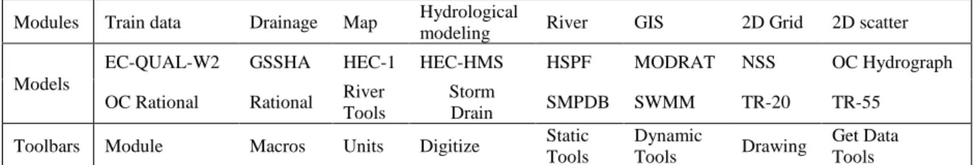
is achievable considering the probability of occurrence. The following contents are offered by module in project explore in mentioned system.
Table 2-1: Provided contents by module in project explorer (WMS manual, AQUAVEO)
Modules Train data Drainage Map Hydrological
modeling River GIS 2D Grid 2D scatter Models
EC-QUAL-W2 GSSHA HEC-1 HEC-HMS HSPF MODRAT NSS OC Hydrograph OC Rational Rational River
Tools
Storm
Drain SMPDB SWMM TR-20 TR-55 Toolbars Module Macros Units Digitize Static
Tools
Dynamic
Tools Drawing
Get Data Tools
It should be noted that the WMS supports 2D hydrological models such as US Army Corps of Engineers (USACE), GSSHA model, and the HMS version of the quasi-distributed MODClark method in order to forecast the flood over 2D domain (WMS manual, AQUAVEO).
What's new in WMS (v10.1)
WMS developer group presents this version of WMS (v10.17(64-bit), updated on March 2018) to the users, by debugging the WMS last version (v10.0.13(64-bit), March 2016) and adding support of some models contains EPANET (water distributed model), EPASWMM (sanitary sewer and storm drain options), time series data calculator, improving HY12 (storm drain and hydrology model), GSSHA model (Better calibration of streams and MWBM (mine water balance model).
Introduction to HEC-RAS (v4.0.1)
Hydrologic Engineering Center-River Analysis System (HEC-RAS (4.0.1)) is designed for one-dimensional and two-one-dimensional river analysis. The river analysis components of HEC-RAS are categorized in: computation of steady flow water surfaces, simulation of unsteady flow states, sediment computation of movable boundary models and water quality analysis (HEC-RAS, manual (v 4.1)). In all four mentioned components, the common geometric data and hydraulic computations routine approaches can be used.
“Steady flow water surface profiles” and “Unsteady flow simulation” are the two important components in this project, described as following:
1- Steady flow water surface profiles: this component of modeling system is considered to calculate water surface profile for steady gradually varied flow, through handling full network of channels or single river bank (HEC-RAS, manual (v.4.1)). This option can model the subcritical, supercritical, and mixed flow regime water surface profile. The fundamental computational method is based on the one-dimensional energy evaluation, which evaluates the energy losses through Manning equation and contraction/expansion (the coefficient which was multiplied by change in velocity head) (HEC-RAS, manual (v 4.1)). The momentum equation is used in rapid water surface change states including hydraulic jumps or river confluence. The computation of effect of obstructions, dams, culverts, and other constructions in floodplains could be considered in this part as well (HEC-RAS, manual (v 4.1)).
2- Unsteady flow simulation: by using this component of HEC-RAS (v4.1), the simulation of one-dimensional unsteady flow of full network channel is possible. The hydraulic calculation of river cross sections, flood water depth, in the unsteady simulation module are included. Hydraulic computations in special states like dam break, pump station, pressurized pipe system and navigation dam are other capabilities of HEC-RAS (HEC-RAS, manual (v 4.1)).
The reason of using this software (HEC-RAS) in this project is Richelieu Flood simulation. By using unsteady flow data and analysis option and applying the boundary conditions according to the available hydrometric station information, the unsteady flow state was simulated, and it was calibrated according to the control station.
HEC-RAS uses finite difference scheme to inject one-dimensional St-Venant equations (mass and momentum conservation laws), could simulate unsteady flow state.
(2-2)(Chaudhry, 2008) Where,
Q is the volumetric flow rate in the channel (m3/s), A is flow area (m2), ql is the flow into the channel from other sources(could be zero), S0 is the channel bed slope (m/m), Sf is the friction slop, v is flow velocity (m/s) and y is flow depth (m), g is the acceleration due to the gravity (m/s2), (Chaudhry, 2008).
Equation (2-1) referrers to the continuity equation with considering that, mass is conserved along any closed contour in the x-t plane if the right-hand side of this equation(ql) is zero (Chaudhry, 2008).
The momentum equation (2-2) which referrers to equation of motion or dynamic equation, involves important terms as follow.
In steady uniform form term (the first term), the slope of the energy grade line (E.G.L) is defined the same as the channel-bottom slope (Chaudhry, 2008). The equation for steady gradually varied flow (G.V.F) is obtained by considering the variation of the flow depth and the velocity head by derivation in distance (x) (Chaudhry, 2008). The third term, the unsteadiness or the local acceleration term is added to make the equation (2-2), valid for unsteady nonuniform flow as well (Chaudhry, 2008).
The important assumptions which were considered to derive the St-Venant equations are in the following (Chaudhry, 2008):
- The flow pressure distribution is supposed hydrostatic (in the streamlines without sharp curvatures).
- The channel bottom slope (s0) is so slight that the flow depth which is measured normal (yn) to the channel bottom or is measured vertically(yp) are almost equal.
- The channel is considered prismatic (the channel cross section and the channel bottom slope(s0) are constant along the distance(x)).
-The head losses(hf) in unsteady flow could be simulated by using the steady state resistance laws, like Manning or Chezy equations, (head losses due to the flow velocity(v) in unsteady flow state are the same as that in steady flow state).
CHAPTER 3
DATA GATHERING
Present chapter will illustrate how recorded information of Richelieu Flood (2011) were prepared to apply in WMS model. Coping with limitations and lack of desirable information will be discussed as well. Details of applied procedure to integrate will clarify in the Followings.
3.1 The case study
The flood occurred in the Champlain Lake and Richelieu River (LCRR) areas at the bi-national border between the United States and Canada, in spring of 2011. This phenomenon drew comprehensive attentions and motivated the development of impacts measures to the implement a flood warning system for the international Champlain watershed(International Joint Commission, 2015).
This disaster occurred as a consequence of snow accumulation in Champlain Lake and severe spring rainfall in the Richelieu River in Saint-Jean-Sur-Richelieu, Quebec (downstream of the lake). This flood resulted in around 88 million dollars worth of damage over 60 sequential days (International Joint Commission, 2015). In the last century, Champlain Lake and Richelieu River faced three other flooding events occurred in 1932, 1972 and 1992. The maximum Champlain Lake water level was recorded 31.477 m (NDGV29) in 2011 by a regional hydrometric station at Rouse Point : latitude (44⸰59’46”N) and longitude (73⸰21’37”) in New York, at 1.7 km from the Canadian-American border approximately (International Joint Commission, 2015). In Champlain watershed, the Jay Peak Mountain received 10 meters of snow in 2011, which was estimated 15% more than the regional annual amount of snow accumulation (International Joint Commission, 2015). Additionally, in March, April and May of 2011, the precipitation was 182 % of normal (measured 1981-2010) (Morrissette Pare, 2014).The first inundation between Champlain Lake and St-Jean-Sur-Richelieu was occurred on April 23, 2011 and it continued until June19, 2011 (Morrissette Pare, 2014).This inundation led to the evacuation of around 2000 local residents from flooded areas in a radius of one kilometer from the Richelieu River banks (Morrissette Pare, 2014). The selected part of Richelieu River for this study is 53 km long with the area of around 73 km2 (Google Earth, 2018) (Figure (3.1)). This part of Richelieu River is mostly straight, and the river bed slope from upstream to downstream is 1.132×10⁻⁴ m/m. The Champlain Lake (with the source
of the Saint-Lawrence River) with an area of 1269 km2 and a length of around 201 km, is located at the border of the United States (Vermont and New York) and Canada (Quebec) (Google Earth, 2018). The Richelieu River is in the east south of Montreal, Quebec, in the Richelieu River watershed. The Richelieu River has area of 2506 km2 and 124 km long, starts from Rouse Point in New York and terminates in Rapid Fryers in downstream of St-Jean-Sur-Richelieu city.
3.2 Background case study
Geographical location
The Richelieu River in Montreal, QC with total length around 130 kilometers flows from Champlain Lake in the United States northward to the St-Lawrence River near St-Pierre Lake. Champlain Lake which is in the bi-national border between Canada and the United States has a watershed area of 19925 km2. The selected studied part of this river with length of 53 km and 72km2 area contains three hydrometric stations from upstream to downstream covers Rouses Point, Marina-St-Jean (St-Jean-Sur-Richelieu) and Rapid Fryer. Rouses Point with latitude (44⸰59’46”) and longitude (73⸰21’37”) is a hydrometric station in the United States in 1.5 kilometers of Canadian-American border records water elevations (Morrissette Pare, 2014). This station was considered as an upstream condition of the studied area. The second station is Marina-St-Jean, a Canadian hydrometric station in Marina-St-Jean-Sur-Richelieu registers water elevation as well (latitude (45⸰18’08”) and longitude (73⸰15’0”)) (Morrissette Pare, 2014). Mentioned station was considered as control station in the simulation process. The downstream condition set is related to Rapids Fryers as a Canadian approximately complete station in the present study for water elevations and water discharges records. Its latitude is (45⸰23’54”) and longitude (73⸰15’30”). The last station was installed in the project of constructing a dam in1939 (which was never operated) with the aim of controlling water levels of Champlain Lake. It should be noted that there are other hydrometric stations in this region: St-Paul-de-Ille-Aux-Noix and Barrage Chambly which were installed after this flood in 2011, therefore their information did not applicable in the present study (Morrissette Pare, 2014). Furthermore, the meteorological regional station in Acadie near the Marina-St-Jean-Sur-Richelieu did not record any snow accumulation during the flood time (April25, 2001-May8, 2011),it just recorded the flash rain over Champlain watershed (Morrissette
Pare, 2014). All of hydrometrical information which was registered by these stations were daily average data, so the daily time- evaluation was not possible.
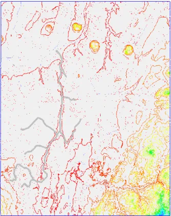
Figure 3.3: Satellite images (NASA,2011): a (before flood), b (during flood), c (infrared image during flood)
3.3 Data gathering and preparation
Geo data base
From the Geo data base (Geo base site, 2014) and the intergovernmental Canadian information, the following information and data were collected:
- Soil covers
- Numerical elevation data (topography) - Satellite images
- Administrative boundaries - Geodesic network (UTM zone8) - National road networks
- National hydrographic networks - Rail networks
Soil cover
Soil cover map produced by Geo base (2009) in different land covers is consisted of different polygons in various colours, which shows the variety of land use. Roughness coefficients were extracted from this soil cover map in this case study( Figure (3.4)) (Morrissette Pare, 2014).
Figure 3.4: Richelieu River material cover map (Morrissette Pare, 2014)
Topographical data
In this case study project, basic terrain data (topographical data) in scatter point forms (x, y, z) was converted to the appropriate type of map in WMS (v10.1) from Richelieu River flood project (by Morrissette Pare, 2014 using SMS).
Satellite image
Satellite images for this case study, Figure (3.3), were taken from NASA satellite images related to the flood in 2011 (before, during and after the inundation). The low resolution of the images was not good enough in order to evaluate some details like distinguishable numbers of houses around the river or clear boundary of forest and urban areas.
Other applied maps
Through other available maps: national hydrographic network, US National Land Cover Database (NLCD), these useful and necessary information were collected:
In the studied area, there is a regional river flow toward Mossisquoi Bay near St-Peul-de-Ille-Aux-Noix named “Riviere de Sud”. It should be noted that in 1972, by constructing a dam in the studied area (Project St-Jean-Sure-Richelieu,1972), some bathymetric data were gathered manually which are not reliable presently (Morrissette Pare, 2014).
Flood recorded information
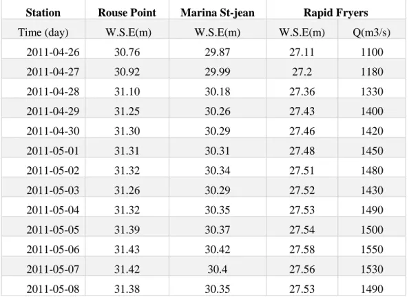
The recorded flood information in three stations (Rous-Point station, Marina-St-Jean station, Rapid Fryers station, along Richelieu River, Quebec) were applied as the basic information to boundary conditions in Richelieu flood simulation (Table (3-1)).
The recorded information in these stations are respectively from upstream to downstream river direction: Rouse Point with recorded daily water surface elevation flood was considered as the upstream condition (stage hydrograph). The second station, Marina St-Jean station, considered as the control station and water surface elevation values of flood were recorded on daily base. These flood elevations data were treated as the observational values. From the third station, Rapid Fryers station, water elevation surface flood values and corresponding water discharge values were extracted. During Richelieu flood, these extracted values were assigned to downstream boundary condition set (rating curve). The water discharge value estimated from downstream water discharge value in the first day of flood (Rapid Fryers) considered as initial condition. In HEC-RAS, the “stage hydrograph” option instead of “flood hydrograph” take into account as a flood upstream boundary condition.
To do this specific, the depression points of recorded stage hydrograph were removed and additional points by interpolation of existing points were added. The flood duration after editing stage hydrograph were 21 days to have the bell-shaped curve and going back to the before-flood river state. Therefore, the adjusted stage hydrograph in a complete bell-shaped curve (Figure (3.5)) was set in HEC-RAS.
The information of third station in downstream including water surface elevation and water discharges used in order to draw the rating curve (Figure (3.6)). Certain corrections applied to this graph by removing the last two points after peak water discharge (1550 (m3/s)) to have a completely rising curve (Figure 3.6).
Table 3-1: Flood recorded data in three hydrometric stations (Morrissette Pare ,2014)
Station Rouse Point Marina St-jean Rapid Fryers
Time (day) W.S.E(m) W.S.E(m) W.S.E(m) Q(m3/s)
2011-04-26 30.76 29.87 27.11 1100 2011-04-27 30.92 29.99 27.2 1180 2011-04-28 31.10 30.18 27.36 1330 2011-04-29 31.25 30.26 27.43 1400 2011-04-30 31.30 30.29 27.46 1420 2011-05-01 31.31 30.31 27.48 1450 2011-05-02 31.32 30.34 27.51 1480 2011-05-03 31.26 30.29 27.52 1430 2011-05-04 31.32 30.35 27.53 1490 2011-05-05 31.39 30.37 27.54 1500 2011-05-06 31.43 30.42 27.58 1550 2011-05-07 31.42 30.4 27.56 1530 2011-05-08 31.38 30.35 27.53 1490
Figure 3.5: The corrected stage hydrograph applied as upstream boundary condition
Figure 3.6: Adjusted rating curve applied as downstream boundary condition
30.7 30.8 30.9 31 31.1 31.2 31.3 31.4 31.5 Wa ter s u rf ace ele vat ion (m ) Flood duration(day)
River water elevation( Rouse-Point station
)
Editing basic geographical information (DEM, TIN)
The basic map of this project contains scatter points derived from SMS (Morrissette Pare, 2014) which was applied for preparing compatible data to exert in WMS (v10.1). Furthermore, by importing scatter points in WMS, geographical coordinates of points were converted to UTM (Universal Transverse Mercator). In this project adjusting image transparency to desirable magnitudes was another important operation.
Digital Elevation Models (DEMs) are the most common available digital elevation sources. DEMs are fundamental input data in WMS for defining watershed characterizations. DEMs are rigid data structures which consist of a two-dimensional array of elevations with constant spacing between elevations in the x and y directions (manual WMS, AQUQVEO).
Rebuilding DEM
By using web service (on-line map command) in WMS, the up-dated DEM(s) of studied area was downloaded. Then by converting DEM(s) to TIN(s) (Triangular Irregular Network(s)), the DEM(s) were retrieved. In rebuilding of DEM(s) process via merging TIN(s), superimposing of two layers (studied area TINs and downloaded ones) was conducted. Then double points were omitted and missed points were rebuilt. Completed DEMs layer from merged TINs was created to use in the project file in WMS.
Merging two or more elevation data layers into a single TIN has three prerequisites. Firstly, the coordinate systems of each set of elevation data should be matched. Secondly, the elevation data was lined up, and all the elevations converted to the same unites: US Customary or SI. Next step was converting each set of elevation data to a separate TIN and final operation was merging all of the TINs (manual WMS(v10.1), AQUAVEO). The last step of map preparations was trimming DEM(s) which could be reduced the computational time in applied basin. In this map, the differences between elevations of created contour lines were very slight that we considered the studied area almost flat with very mild slope.
Figure 3.7: Background map with mild contour lines and stream networks, Richelieu watershed, 2017
3.4 One-dimensional model characterization
Defining project in WMS
The following step in the WMS (v10.1) is defining project bounds to implement the watershed containing river model. Setting mentioned project in WMS with following details in Table (3-2) to delineate watershed details and corresponding stream network was the next step.
Table 3-2: Project details
Projection Zone Datum Planar unite
Horizontal
MTM (eastern Canada) 8 (75.0w-72.0w) NAD 83 meter
Specifying river banks
For defining the Richelieu River in the WMS, the left and right river banks and river centerline should have been defined. This important was done by using infrared image, NASA image (which were not very clear) and on-line map (world imagery) on background (Figure (3.8))
Figure 3.8: Right and left Richelieu River banks in studied area
Creating cross sections
In one-dimensional modeling methods, defining cross sections along rivers is a fundamental operation to delineate the river plan in corresponding software. In this project, all information about background maps, river and material flood plains assigned in each cross section. Richelieu River, which is not a meandering river (in this selected part), with a length of 53 km and 113 cross sections, by the aim of covering almost all details over the river length and observing the all challenging positions, was defined in WMS. The distance between created cross sections was not constant. In every 400-500 meters along the river length, one cross section was defined to assign into corresponding coverage. Some following key points in creating cross sections to consider: - All cross sections should be perpendicular on defined center line.
- Cross sections (from upstream toward downstream) should not cross each other. - The cross sections were made from left side to right side.
- The cross sections were extended from the first point in the left bank to the furthest point of Right Bank (this factor was not mentioned in the manual, but we take into account in this project). - Cross sections should not cross each river bank line more than once.
The maximum allowable number of material properties which are assigned in each cross section is 20 in all composed 500 points, so this limitation was applied in assigning cross sections. Other options like geometric data, line and point properties, were edited for every single cross section.
Defining centerline
The first try for specifying river centerline was done by drawing a line between two riverbanks in the minimum elevation in centerline coverage of map data. Then by assigning every cross section to corresponding data base, the centerline was adjusted to the proper river thalweg in auto mark option. The Richelieu River was divided into three parts regarding to three hydrometric stations (Rous-Point station, Marina-St-Jean station, Rapid Fryers station, along Richelieu River, Quebec) in the studied area. The third part of river located between Marina-St-Jean station and Rapid-Fryers station was divided into left and right sections, based on the specific regional morphological river changes.
For introducing this specific part of river into WMS, additional centerline is not allowed in the one-dimensional modeling approach (Figure (3.8)).
The one-dimensional schematic river map (Figure (3.9)) which was made of both 113 extracted cross sections and adjusted Richelieu River thalweg were exported to HEC-RAS.
Figure 3.9: One-dimensional Schematic Richelieu River in HEC-RAS
Material coverage
In this project each model layer in WMS (v10.1) was defined in separated coverages. Every polygon material was specified in background maps (NASA image, world imagery map and soil cover map) and each polygon was assigned to its corresponding coverage.
The material of background areas in WMS are categorised into field, forest, dense forest, very dense forest, urban, and river areas. Every material polygon with its specific colour was assigned to corresponding relevant roughness factor (Figure (3.4)).
Roughness coefficient
Roughness coefficient is a key factor in hydrodynamic modeling research subjects. River and flood plain Roughness factor represents the resistance of material to flows in natural and artificial channels and flood plains (Chow, 1959).
In Manning's formula, “n“as a roughness factor was presented in Open-Channel Hydraulics (Chow, 1959) book .
𝑉 = 1 𝑛 𝑅
.6 𝑆𝑒.5 (3-1) (Chow, 1959) Where,
V= mean velocity of flow (m/s) R= hydraulic radius (m)
Se= energy grade line slope (m/m), and n= Manning's roughness coefficient (s/m1/3).
To calculate the roughness factor in rivers and flood plains, following adjusted elements were utilized (Chow, 1959):
- Degree of irregularity of surface flood areas (ratio of width to depth) - Meandering degree (variation in channel cross sections)
- Obstructions (various in size and shape)
- Vegetation which depends on the depth of flow, the percentage of the wetted perimeter covered by the vegetation, and the density of vegetation below the high-water line.
The final values after applying adjusted factors was recorded in Table (3-4) for natural channel and corresponding flood plains.
According to the Table (3-3), appropriate material to corresponding polygons was assigned to the existing material covers modeling layer. In the existing cover map ((Figure (3.4)) Richelieu River material cover map (Morrissette Pare, 2014)), materials categorized in eight groups: forest (green),
dense forest (dark green), very dense forest (double dark green), urban area (yellow), field (gray) and Richelieu River in third parts (blue) with different colours to differ (Table (3-3)).
Table 3-3: Roughness coefficients of Richelieu River and flood plains
Material Roughness coefficient (Chow, 1959)
Quebec (1972)
min max
Urban 0.04 0.06 Rouse Point-St-Paul 0.025
Field 0.03 0.04 St-Paul-Marina-St-jean 0.03
River (three parts) St-Jean- Rapid Fryer 0.03
Forest 0.03 0.05
Dense forest 0.05 0.08
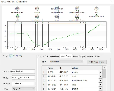
Figure 3.10: Sample cross section of Richelieu River (station:16465.5) assigned to WMS
The geometric plan of Richelieu River and watershed was exported to HEC-RAS in order to make hydraulic computations and flood simulation.
CHAPTER 4
METHODOLOGY
The procedure which was applied in methodology part of this thesis, started by applying WMS (v10.1) to make the Richelieu River and watershed geometric plan. Then followed by simulated Richelieu flood using HEC-RAS (v4.1) and continued by probabilistic method which was used in WMS (v10.1) to predict the probabilistic flooded area.
Richelieu watershed (selected part) based on geographical data, satellite images and on-line maps was delineated using WMS(v10.1). Number of cross sections were drawn and extracted over the 53 km of Richelieu River. Assigning each cross section in an appropriate layer corresponding roughness coefficient (Quebec, 1972) was done. Then according to the material cover map (Figure (3.4)), this study area includes Richelieu River and floodplains using separated polygons, were assigned to the model. Exporting to HEC-RAS (v4.1) was the following step to simulate Richelieu Flood (2011).
Next step is model calibration based on appropriate roughness coefficients of river bed and floodplain. First trial for model calibration using automatic HEC-RAS calibration option did not respond to this model, so accurate parameter estimator: PEST, was applied to calibrate this model. HEC-RAS output file as a binary file (not readable), led us to apply GSTARS (v3.0) (Generalized Sediment Transport model for Alluvial River Simulation). By using GSTARS, input text files of PEST were prepared and applied to run. According to the approximately steady part of flood information in upstream and downstream hydrometric stations, model calibration using PEST was done.
Calibrated roughness coefficients were used to flood simulation using HEC-RAS (v4.1). Richelieu flood was simulated by applying corresponding boundary conditions. The last part by referring to WMS was extracting probabilistic flooded areas based on Monte Carlo simulation method. Following flow chart demonstrates mentioned methodology in desirable details.
Figure 4.1: Methodology diagram WMS (Geometric plan)
Model calibration
PEST (Roughness coefficient calibration)
HEC-RAS (Flood simulation by calibrated coefficients)
WMS (Probabilistic flooded areas using Monte Carlo
method)
GSTAS (Input file preparing) HEC-RAS (Automatic calibration roughness no
CHAPTER 5
NUMERICAL MODELING
Applied numerical method to simulate Richelieu flood and extracting flooded areas is explained in current chapter. To do this, at first model calibration will describe. Then, flood simulation using HEC-RAS with unsteady flow option will clarified. Finally, applying Monte Carlo method in extracting probabilistic flooded areas will demonstrate.
5.1 Model calibration
Via calibration, model-generated values should be adjusted to the observed values in calibration process. Observed values are obtained by experimental methods or recorded values should be applied in calibration, in order to result in adequate confident deference degree. By minimizing differences between observed and generated values, model will represent the system’s behaviour properly. The applied model parameters need to be adjusted until the model-generated values fit to observed value(s) as closely as possible. Then, a model could be referred as “calibrated” with minimum uncertainties.
By considering the sensitivity of roughness coefficients in hydrodynamic models (flood simulation, river modeling or flood plain delineations), dependent hydraulic parameters to this specific coefficient became clear. The most known dependent values to roughness coefficients are water discharges and water surface elevations in hydraulic engineering researches. Calibrating “n” factor to an acceptable confident range based on relevant materials could greatly increase the hydraulic model precision.
In present case study, the first trial of Manning coefficient calibration method done by HEC-RAS. Automatic roughness coefficient option was defined in HEC-RAS as an option of unsteady flow state by corresponding a number of applied requirements including observed value in specified cross section(s), methods of estimating error (squared and averaged), number of iterations and specified flow roughness. The result of this option (calibrated roughness coefficients) was not in acceptable range to reach control water surface elevation at 30.30 m. Therefore, not satisfied responding of HEC-RAS calibration option to this model led us to apply PEST as an optimiser software with capability of supporting every model.
Since the HEC-RAS output file is not readable by PEST (binary file), with the aid of GSTARS (v.3.0) (Generalized Sediment Transport model for Alluvial River Simulation) all of watershed and river data were transferred to the text file for running in GSTARS (v.3.0). This software is the most recent version of series of numerical model for simulation of water and sediment transport in alluvial rivers was developed at the US. Bureau of Reclamation, Denver, Colorado (GSTARS v.3.0manuel).
5.2 GSTARS (v.3.0)
The numerical model (GSTARS) which could solve complex river engineering problems, has great capabilities and limitations namely:
- Computation of hydraulic parameters in open channel flow (fixed or movable boundaries), with or without sediment transport, alsoestimation of water surface profile in subcritical, supercritical, and mixed flows
- Simulate hydraulic and sediment variations in two longitude and transvers directions with the limitation of applying to varied and unsteady conditions.
Preparing GSTARS input file
In input file of GSTARS (v.3.0) the information of each cross section along the Richelieu River in the appropriate GSTARS format is in the Table (5-1). According to the flood information recorded in Table (5-1): by selecting the 48 hours (April30, 2011(00: 00) till May1, 2011(24:00)) as an approximately constant state during flood occurrence, was applied in GSTARS. Marina St-Jean as a control station by average water elevation during mentioned 48 hours: 30.30 m, applied as an only control measured point for calibration process.