A conditional approach to hedge fund risks

A conditional

approach to hedge fund

risk

Florent Pochon

Jérôme Teïletche

Correspondence should be sent to: IXIS CIB Research Department 47 quai d’Austerlitz

75648 Paris Cedex 13 France

E-mail: [email protected], [email protected]

Phone: 33 (0)1 58 55 14 69, 33 (0)1 58 55 14 94

Abstract :

In this study, we apply a two-step conditional Bayesian approach to hedge fund risk. In the first step, a mixture of two normal distributions is estimated for a core asset, one distribution being identified as linked to a “quiet” regime, the other one to a “hectic” regime. The conditional probabilities of each regime are then inferred and a mixture of distributions is deduced for peripheral assets. In our application, the core asset is alternatively chosen as the S&P index or the Baa/Treasuries yield spread and the peripheral assets are the major hedge funds strategies over the period 1990-2004.

The methodology has several advantages given specific features of hedge funds returns, notably non- linear exposure to standard assets returns and short sample history. We identify significant changes in the distribution (mean and standard deviation) of hedge fund returns across regimes. Results are less clear-cut for the correlation with standard assets, as modifications can be imputed to a certain extent to a form of selection bias. We finally present an application of the methodology for stress tests on hedge funds portfolios.

Risk is one of the fundamental elements of the analysis of hedge funds. On the one hand, as hedge funds are characterized by partial exposures to the markets on which they intervene (for instance, Long-Short strategies), their risk evaluated by standard deviation or any other measure that is partly linked to it (VaR, etc.) is lower than that related to a simple buy-and-hold position on the underlying assets1. On the other hand, several recent episodes such as the bankruptcy of the LTCM fund have shown that this low risk could be merely apparent. While there is undeniably a fundamental operational risk dimension, these incidents also express the unique nature of hedge fund risk. In particular, hedge funds present non- linear exposures to standard assets (Argawal and Naïk [2004], Fung and Hsieh [1997, 1999, 2001, 2002, 2004], Mitchell and Pulvino [2000])2. These non- linear exposures partly account for the non-Gaussian (asymmetrical and leptokurtic) nature of the distributions of hedge funds returns which is characteristic of assets with a significant extreme loss risk (Brooks and Kat [2003]).

Taking into account this non- linearity is fundamental in the risk management of hedge funds. One way is to incorporate it in a factor model, by introducing threshold effects or reproducing payoffs of options on the principal underlying asset. It is, however, difficult to project such models, notably when predicting the probabilities of extreme events. An alternative approach is to suppose that the returns on hedge funds are derived from a regime-switching model. While the limited track record of returns makes it difficult to estimate highly parameterized models such as Markovian processes3, one can envisage a mixture of normal distributions as this type of model is perfectly able to reproduce the non-Gaussian characteristics of empirical distributions of financial assets and its use in risk management is well established (Zangari [1996]).

Kim and Finger [2000] propose an application of this model to conditional multivariate analyses. More specifically, they estimate initially a mixture of normal distributions for a core asset, meant

to act like a catalyst for the state of the market, and deduce the respective probabilities of being in a quiet regime or in a hectic regime; subsequently, they study the behaviour of non-core assets in each regime. In this way, we also obtain a mixture of normal distributions for all the non-core assets — and therefore a potentially asymmetrical and leptokurtic distribution — by restricting the modelling to the core asset. One can notably test whether the behaviour of non-core assets (mean, standard deviation and correlation with the core asset) is modified significantly during hectic phases, a major issue in terms of risk management or asset allocation. In this article, we propose applying such a model to the analysis of hedge funds returns. This presents several advantages. First, it leads to a simple specification likely to reproduce the non-linearity in the relationship between hedge funds returns and standard assets ones. Second, it partly offsets the lack of historical hindsight for the analysis of hedge fund risk since the regimes of core assets can be estimated separately over a longer period4. Finally, the simplicity of the framework offers the possibility of implementing easily stress scenarios, usually difficult to implement for hedge funds because of the lack of observations.

In the case of hedge funds, the choice of core assets is complex because investment possibilities are wide and flexible over time and across strategies: equities, bonds, FX markets, commodities, etc. We chose two key underlying assets: the equity market and the corporate bond market. In both cases, they are two favoured investment vehicles of hedge funds (Fung and Hsieh [2004]) and more generally, they are accurate mirrors of the state of the economy. More precisely, we rely on monthly S&P 500 index returns and monthly changes in the gross spread between the Moody’s Baa corporate bonds rate and the long-term government bonds rate over the period from January 1925 to August 20045.

The rest of this paper is organised as follows. Section 1 presents the estimate of the mixture for the core assets. Section 2 analyses the implications for the returns on hedge funds, both on the mean and the standard deviation then on the correlation with core assets. Section 3 presents an application of the methodology to stress tests. Section 4 outlines our conclusions.

1. Estimation of the mixture for core assets

As a first step, the methodology requires to estimate a mixture of distributions for the core asset returns, each distribution being interpreted as “regimes”. In this paper, we follow Kim and Finger [2001] and concentrate on a mixture of two normal distributions, a solution which offers a satisfactory arbitrage between parsimony and adjustment quality.

Let us have x the value in t of the core asset andt s ,t st =1,2, a random latent variable that stands for the regime that prevails in period t . The unconditional density of x is given by_t 6:

(

x_t;θ

)

=ω×Φ

(

x_t s_t =1;θ

)

+

(

1−ω

)

×Φ

(

x_t s_t =2;θ

)

f , (1)

where Φ

(

x_t s_t =1;θ

)

≡Φ

(

x_t;µ₁,σ₁2

)

stands for the normal distribution, with mean µ and ₁ variance σ , associated to the first regime and ₁2 Φ

(

x_t s_t =2;θ

)

≡Φ

(

x_t;µ₂,σ₂2

)

stands for the normal distribution associated to the second regime, with mean µ₂ mean and variance 2

2 σ .

(

2

)

, ;µ σ t x

Φ is the density of normal distribution:

(

)

(

)

        − − = Φ 2 2 2 2 exp 2 1 , ; σ µ σ π σ µ t t x x . (2)

θ , θ

{

µ ,σ ,µ2,σ22,ω

}

2 1 1

= , stands for the vector of parameters to be estimated, with ω the mixture parameter.

A natural interpretation of the mixture in the case of financial markets is that of a mixture of a hectic regime with a quiet regime. We suppose that the hectic regime is associated to the first distribution. In this case, we expect ω to be less than 0.5 and rather small, 22

2 1 σ

σ > and µ₁ <µ₂ if x stands for returns or t µ1 >µ2 if x stands for yield spreads. t ω is thus the unconditional probability of being in the hectic regime and

(

1−ω

)

the probability of being in the quiet regime.

It is well known that the estimation of (1) is tricky since the (unconstrained) global maximum of the log- likelihood,

( )

=

∑

T₌

(

)

t f xt

LL

1log ;θ

θ , does not exist. Indeed, a problem occurs if we

suppose that one of the distributions has a mean exactly equal to one of the observations with a nil variance since the log- likelihood then becomes infinite and “maximised”. Therefore, we exclude this specific case by constraining all the variances to be different from zero. We furthermore carry out various estimates by changing randomly the initial values. In each case, we apply the EM algorithm (Hamilton [1994, pp. 688-689]).

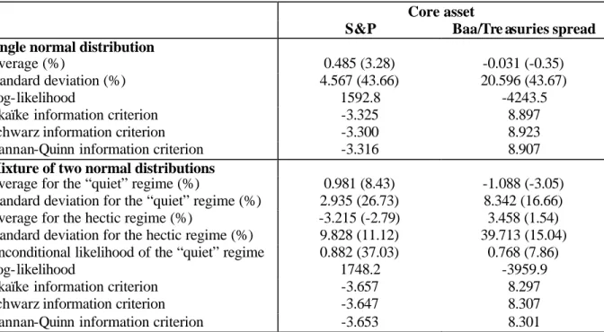
Table 1 reports the results of the estimation of the mixture obtained for the two core assets. As expected, the unconditional probability of the hectic regime is far lower than 0.5 (in fact, it is lower than 25% in both cases), the variance is higher and the mean lower in the case of S&P returns and higher in the case of the Baa spread changes. Visual inspection of the distribution (not reported to save space but available on request) shows that the mixture of distributions offer a far better fit than the one obtained through a single distribution. More formally, we evaluate the

relevance of the mixture using standard likelihood ratio tests. As reported in Table 1, the null hypothesis is very easily rejected, meaning that the mixture leads to far better modelling of core assets returns than the single normal distribution. However, one has to be cautious since with mixtures of distributions, likelihood ratio tests do not satisfy standard regularity conditions. Thus, as can be seen in Table 1, we also rely on various information criteria: they prove systematically smaller in the case of the mixture, confirming the superiority of the mixture over the simple distribution.

Once the mixture is estimated, we can reverse the problem and deduce, conditionally on the realisation of the core asset at a given date, what is the probability of being in either regime. Formally, these ex post conditional probabilities are given by:

{

θ

}

ω

(

₍

_θ

₎

θ

)

; ; 1 ; 1 Pr t t t t t x f s x f x s = = × = , (1a)

{

θ

}

(

ω

)

(

₍

_θ

₎

θ

)

; ; 2 1 ; 2 Pr t t t t t x f s x f x s = = − × = . (1b)

By calculating (1a) and (1b) for each observation period, we obtain a time series of the ex post probability associated to each regime. Chart 1 represents the results of this calculation for the hectic regime for the two core assets. The conditional probability of a crisis for the S&P was very high in 1929 and in the thirties, in the run- up to World War II, in the wake of the first oil shock in 1974 and in 2001-2002. For the Baa/Treasuries spread, the conditional probability of a crisis was also high in 1929 and in the thirties, around the time of the Korean War (1956-58) and has been steadily high since 1966, with noteworthy peaks in 1974, 1980-82 and 2001-02. All in all, while the two core assets unsurprisingly present common sensitivity to periods of major

economic and financial shocks (the Great Depression, the oil shock, the technology bubble), both also show specific stress periods.

2. Implications for hedge funds returns modelling

2.1. Methodology and data

Generally speaking, we can consider that the regimes observed on the core asset reflect the regimes that influence overall the economy and all financial assets. In particular, we can use the conditional probabilities of being in either regime according to the core asset and compare it with returns on another financial asset (named “peripheral”) to deduce the specific features of this asset in the different regimes (Hamilton [1994], Kim and Finger [2000]). More specifically, we can infer estimates of the different moments of peripheral assets conditionally on the regime observed for the core asset. Formally, if we denote _{ys i}

t=

,

µ the mean of returns on asset y when the core asset is in regime i, a natural estimator is the following:

{

}

{

}

∑

∑

= = = = × = = _T t t t T t t t t i s y x i s y x i s t 1 1 , ; Pr ; Pr θ θ µ . (2a)

The conditional mean is therefore built as a weighted mean of observations of returns on asset y with weights calculated as the conditional probabilities of being in either regime according to the core asset. The same calculation can be carried out on higher-order moments. In particular, we deduce conditional variance and correlation, denoted _y2_{,s i}

t=

σ and _{xys i}

t=

,

{

}

(

)

{

}

∑

∑

= = = = = − × = = T t t t T t i s y t t t i s y x i s y x i s t t 1 1 2 , 2 , ; Pr ; Pr θ µ θ σ , (2b)

{

}

(

) (

)

{

}

∑

∑

= = = = = = = = × × − × − × = = T t t t i s x i s y T t i s x t i s y t t t i s xy x i s x y x i s t t t t t 1 2 , 2 , 1 , , , ; Pr ; Pr θ σ σ µ µ θ ρ , (2c) where _{xs i} t= , µ and _x2_{,s i} t=

σ stand for the mean and the variance of x in regime i.

Once the conditional moments are obtained, we can moreover test the significance of changes in correlation levels between the two regimes. This issue is crucial both in terms of risk management and asset allocation. In particular, if we obtain a significantly different distribution in each regime, this suggests that the allocation of wealth calculated in the unconditional case (in other words without drawing a distinction between the regimes) will probably be sub-optimal and will expose to losses. To carry out the tests, we use methods drawing on Monte Carlo simulation, following Kim and Finger [2000]7. The first simulation assumes that x and y are distributed according to a simple multivariate normal distribution and not according to a mixture. This simulation is applied to the mean and to the standard deviation. For these two statistics, we obtain a distribution on the basis of 5000 simulations, from which we evaluate the significance of modifications in all regimes in comparison with unconditional values8.

In the case of the correlation, we specifically carry out two other types of simulation. First, we posit the null hypothesis as characterized by returns on the core asset and those on hedge funds being derived from a mixture of two normal bivariate distributions with a different mean and variance but with an equal correlation in the two distributions9. We thus seek to test whether the

modification in the distribution in the two regimes results from a modification in the first two moments only or also from the correlation with the core asset. Then, we modify the simulation to take into account the potential selection bias that exists when we calculate the statistics by conditioning them on the regime of the core asset. Boyer, Gibson and Loretan [1999] illustrate very clearly this selection bias by showing that the correlation coefficient obtained when the sample is truncated according to the level of volatility seems to change, even when it is maintained equal between sub-samples10. The approach drawn upon here (in 2a, 2b and 2c) is a “smoothed” form of sample splitting, since the separation used is duly partly based on the levels of volatility, each regime being characterized by a significantly different volatility. Although Kim and Finger [2000] point out this potential effect, the y do not specifically address the issue in their significance tests since the y rely on the first type of simulation. We thus propose an alternative simulation to analyse the extent to which our results depend on our truncating process. We split the sample of simulated returns (once more under the null hypothesis of a bivariate mixture with a single correlation in the two regimes) by classifying them according to absolute value. We thus compare the correlation in the quiet regime with the correlation obtained for the

( )

x,y pairings corresponding to the

(

1−ω

)

T lowest absolute observations of x. By contrast, we compare the correlation of crisis with the correlation obtained for the

( )

x,y pairings corresponding to the ωT highest absolute observations of x. While this way of proceeding is somewhat extreme, it allows us to gain information about the importance of the selection bias in the analysis of the correlation.

As for peripheral assets, the application is based on the two main types of hedge fund indices provided by the Hedge Fund Research (HFR) and Crédit Suisse First Boston Tremont (CSFB-T) indices. The two indices are non- investable and present several biases 11 but they are unchallenged references given their public nature and their historical depth. In this study, we

analyse the case of global hedge funds indices and strategy-based indices. The HFR and CSFB-T indices differ according to several dimensions: (1) their historical depth, as the HFR indices generally go back to 1990, and the CSFB- T indices to 1994; (2) their mode of weighting of funds, with an equal weighting for HFR indices and a weighting by the amount of managed assets in the case of CSFB-T indices; (3) entry conditions (duration of track-record, minimum assets, etc.).

2.2. Analysis of the mean and variance

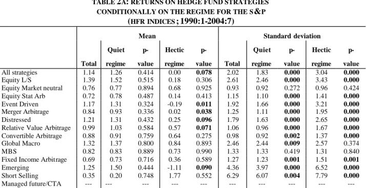
Tables 2A and 2B show the means and standard deviations of hedge funds returns for the various strategies in the case of HFR and CSFB-T indices, respectively. Each time, the p- values stand for the probability of wrongly rejecting the null hypothesis of equality in means or standard deviations with its unconditional value. We will consider that there has been a significant change in the statistic when the p- value is lower than 10% (0.1), a case we single out by highlighting the p-value in bold type.

As expected, we can see that in most cases the mean of returns on hedge funds are lower when the stock market is in its hectic regime. The average difference between the unconditional mean and the hectic regime’s mean is 0.60% per month for the HFR indices and 0.40% per month for the CSFB-T indices. The only strategies to be spared from this decline during the hectic regime are the Short Selling, Equity Market Neutral (in the case of the CSFB-T index only) and CTA/Managed Future ones. While in the first case, the result is totally logical, in the two other cases it can be partly explained by the fact that they are strategies that do not present any long bias to equities. All in all, mean returns are significantly smaller in the hectic regime for 6 indices out of 14 for the HFR and for 3 indices out of 12 for the CSFB-T. On the contrary, it can be seen that all the p-values are higher than 10% in the case of the quiet regime, which means

that the conditional means are not significantly different from their unconditional values. Regarding the standard deviation, the results are straightforward with a rise in volatility in the case of the hectic regime and, by opposition, a fall in volatility during the quiet regime. In the two regimes, standard deviations are significantly different from their unconditional value for virtually all strategies.

All in all, the regimes identified on the US stock market duly seem to lead to differentiated regimes for the returns of most hedge funds strategies. The hypothesis of a mixture of distributions rather than a single distribution appears acceptable in most cases, with at least differentiated variances. Chart 2 illustrates the implication of this result for the HFR index of Event Driven funds if one assumes as before that the marginal distributions are normal ones as previously. We see significant differences for each distribution, the distribution being associated with the hectic regime being far more flattened and with a lower mean than that of the quiet regime. The mixture produces an asymmetrical, fat-tailed and peaked distribution which is typical of hedge funds returns distributions. Still for the Event Driven index, this point is further illustrated in Chart 3 where we contrast the mixture of distributions and a single normal distribution thus obtained with the “true” empirical distribution, the fit being far better in the former case.

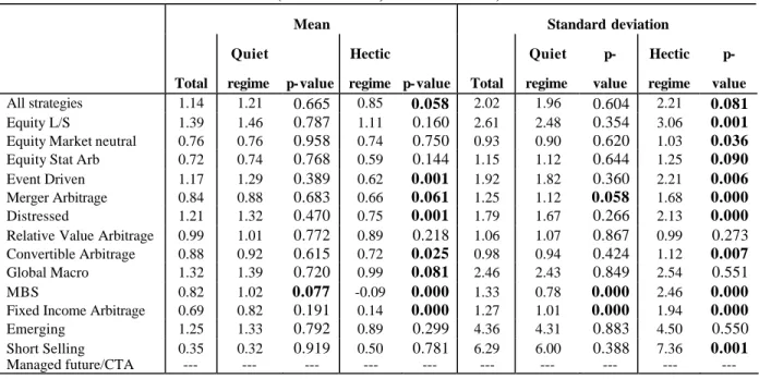
Tables 3A and 3B present the equivalent results whe n the Baa/Treasuries spread is used as the core asset. In most cases, we see a significant fall in hedge fund returns when the credit market is in hectic periods. The only exceptions are again the Short Selling (HFR index), the CTA and the Equity Market Neutral (CSFB-T index). In virtually all cases, the hectic regime is also reflected by greater volatility in returns on hedge funds. Thus, we can see, as for the stock market, a pronounced impact of the core asset regime on hedge fund returns. This result logically confirms

the correlation between credit spreads and stock market volatility (see, for example, Campbell and Tasker [2000]). An interesting difference though with the results for the S&P is that the significant modifications are generally observed both for the first and the second moments while only the latter is observed in the case of the S&P. In other words, whereas the return on hedge funds’ strategies could be represented as a mixture of two normal distributions but where only the standard deviations differ in the case of the S&P, a mean distinction seems also necessary with the Baa / Treasuries spread.

2.3. Analysis of the correlation

We finally apply the same pattern to the coefficient correlation according to equation (2c). From a risk management point of view, the correlation structure is fundamental. Basically, if the correlation becomes higher (in absolute value) during hectic periods, the portfolio will be more exposed than initially expected and the “diversification” effect will tend to disappear when it is most needed.

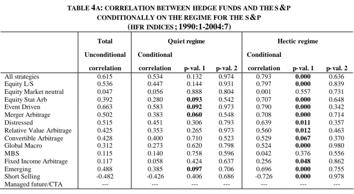
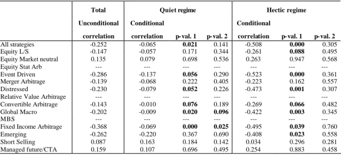
Tables 4A and 4B (respectively, 5A and 5B) show the results obtained in the case of the HFR and CSFB-T indices when the core asset is the S&P (respectively, the Baa/Treasuries spread). Note that here we have two p-values because we have carried out two simulations: both impose the null hypothesis according to which the population is drawn from a mixture of two normal bivariate distributions with different parameters with the exception of the correlation, but the second one takes into account the potential selection bias linked to the conditional approach on the regimes.

The correlation changes significantly when it is conditioned on the regimes. As expected in the hectic regime, the correlation becomes more positive in the case of the S&P and more negative in the case of the BBB spread. This gives ground to concern with respect to the risk management of a portfolio of hedge funds. More precisely, the main modifications are obtained when the S&P is picked as the core asset and with the HFR indices. The statistical significance of these results nonetheless depends on simulation hypotheses. With the conventional simulation, most correlations of strategies turn significantly higher in the hectic regime.

This result is however largely challenged by the second type of simulations. It also appears that it is absolutely common to observe similar "apparent" modifications in the correlation when we condition the sample according to the level of volatility. We have mentioned previously that this type of simulation is probably extreme given the fact that we have not conditioned as explicitly but in a rather smoothed manner. Our results however show ultimately that the change in correlation levels could partly result from a selection bias similar to the one identified by Boyer et al. [1999]. Note consequently that the standard result according to which the slope in a regression of hedge funds returns on stock market returns is non- linear (piece-wise regressions) is more probably due to a modification in standard deviations than a modification in the correlation itself.

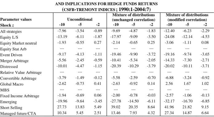
3. An application to stress tests

To finish with, we present in this section an application of the framework to stress scenarios. To save space, we only present examples related to the S&P. More specifically, we calculate expected returns for hedge fund strategies conditionally on a given shock for the S&P. The shock, denoted by z is expressed as a standardized return in excess of the average. To measure the t

impact of this shock, we use the standard formula of conditional expectation in a Gaussian linear problem, that is:

( )

yt xt y yzt

E =µ +ρσ . (3a)

In equation (3a), the parameters are not linked to a particular regime and we restrict its use to the unconditional case reported below for matter of comparison. On the contrary, the approach here retained states that the parameters (mean, standard deviation and, with less confidence, correlation) significantly changes with the core asset regime. To incorporate this fact, we substitute (3a) by the following:

( )

_∑

{

}

(

)

= = = + × = = 2 1 , , ; Pr i t i s y i s y t t t t x s ix z y E t t ρσ µ θ . (3b)

( )

_∑

{

}

(

)

= = = = + × = = 2 1 , , , ; Pr i t i s y i s xy i s y t t t t x s ix z y E t t t ρ σ µ θ . (3c)

The difference between (3b) and (3c) is that the former consider that the correlation remains unchanged in both regimes while in the latter we relax this assumption. We use both hypotheses because our results in section 2.3 as regards the significance of correlation change are not clear-cut. Tables 6A and 6B show the results of the application of the above formula for three alternative stress scenarios for the S&P shock (expressed as units of standard devia tion):

2 , 5 , 10− − − = t

z . Using historical figures over the period 1925-2004 (see Table 1), these four shocks correspond to S&P monthly returns of the S&P: –45.2%, –22.4% and –8.6%. Note that the corresponding conditional probabilities of the S&P being in an hectic regime are 100%,

Results are unambiguous. Expected losses are substantially larger when the mixture approach is used, as opposed to a standard unconditional approach (obviously these turn out into larger expected gains for CTA and Short Sellers). This is all the more true as we allow the correlation to differ across regimes. All in all, the results make clear that the regime approach is not only statistically relevant but also truly valuable in terms of risk management since relying on a simple unconditional analysis may strongly underestimate losses in stress periods.

4. Concluding remarks

In this study, we apply the methodology of Finger and Kim [2000] to hedge funds’ returns. We believe this methodology is particularly well adapted in this context. First, it deals with the non-linearity that is frequently highlighted between hedge funds returns and standard assets returns. Second, this approach circumvents the issue of small sample size in hedge funds data. Since we first separately identify the regimes on core assets (hectic and normal), we indeed use longer historical data than the hedge fund industry and reach greater precision in the estimation of parameters. Lastly, the approach enables us to simulate hedge fund risk and implement stress scenarios within a parsimonious framework.

We have shown that for most strategies, significant modifications are observed (in the expected direction) in distributions of hedge fund returns (via the mean and/or the standard deviation) depending on the regime — normal or hectic — prevailing in the stock market (S&P) or in the credit market (Baa/Treasuries spread). As a consequence, the analysis of market risk of hedge funds is significantly improved by taking into account the regime-switching feature of the core

assets. On the other hand, we have shown that the change in the correlation with these core assets observed in the data partly reflects a selection bias, an issue that Kim and Finger [2000] do not properly address. Interestingly, our results point that the non- linearity observed between hedge fund return and standard assets returns could primarily stem from a change in standard deviations and not from a modification in correlations. Given the importance of these non- linear factors in the risk management for hedge funds, this point would deserve to be studied more in depth. An interesting extension of this study would be to compare the risk measures suggested by this study (for example, the standard deviation in the hectic regime) with the conventional measures (standard deviation or VaR) drawn from the unconditional distribution of returns.

References

Agarwal V., Naik N., 2004, Risk and Portfolio Decisions Involving Hedge Funds, Review of Financial Studies, vol. 17, 1, pp. 63-98.

Boyer B., Gibson M., Loretan M., 1999, Pitfalls in Tests for Changes in Correlations, International Finance Discussion Papers, n°597, Board of Governors of the Federal Reserve System.

Brooks C., Kat H.M., 2002, The Statistical Properties of Hedge Fund Index Returns and their Implications for Investors, Journal of Alternative Investments, vol. 5, 2, pp. 26-44.

Campbell J., Tasker G., 2003, Equity Volatility and Corporate Bond Yields, Journal of Finance, vol. 58, pp. 2321-2349.

Chan N., Getmanski M., Haas S., Lo A., 2005, Systemic Risk and Hedge Funds, NBER Working paper, n°1120.

Fung W., Hsieh D., 1997, Empirical Characteristics of Dynamic Trading Strategies: The Case of Hedge Funds, Review of Financial Studies, vol. 10, 2, pp. 275-302.

Fung W., Hsieh D., 1999, A Primer on Hedge Funds, Journal of Empirical Finance, vol. 6, pp. 309-331.

Fung W., Hsieh D., 2001, The Risk in Hedge Fund Strategies: Theory and Evidence from Trend Followers, Review of Financial Studies, vol. 14, 2, pp. 313-341.

Fung W., Hsieh D., 2002, Asset-based Style Factors for Hedge Funds, Financial Analysts Journal, vol. 58, 5, pp. 16-27.

Fung D., Hsieh D., 2004, Hedge fund benchmarks: A Risk-Based Approach, Financial Analysts Journal, 60, 5, pp. 65-80.

Hamilton J., 1994, Time Series Analysis, Princeton University Press.

Kim J., Finger C., 2000, A Stress Test to Incorporate Correlation Breakdown, Journal of Risk, vol. 2, 3, pp. 6-19.

Merton R., 1981, On Market Timing and Investment Performance I: An Equilibrium Theory of Value for Market Forecasts, Journal of Business, 54, pp. 363-406.

Mitchell M., Pulvino T., 2001, Characteristics of Risk in Risk Arbitrage, Journal of Finance, 56, pp. 2135-2175.

Wang J., 2001, Generating Daily Changes in Market Variables Using a Multivariate Mixture of Normal Distributions, in B.A. Peters, J.S. Smith, D.J. Medeiros and M.W. Rohrer (eds), Proceedings of the 2001 Winter Simulation Conference, pp. 283-289.

Zangari P., 1996, An Improved Methodology for Measuring VaR, RiskMetrics Monitor, Second quarter, pp.7-25.

TABLE 1. ESTIMATION OF MIXTURES OF NORMAL DISTRIBUTIONS FOR CORE ASSETS

Core asset

S&P Baa/Tre asuries spread

Single normal distribution

Average (%) 0.485 (3.28) -0.031 (-0.35)

Standard deviation (%) 4.567 (43.66) 20.596 (43.67)

Log-likelihood 1592.8 -4243.5

Akaïke information criterion -3.325 8.897

Schwarz information criterion -3.300 8.923

Hannan-Quinn information criterion -3.316 8.907

Mixture of two normal distributions

Average for the “quiet” regime (%) 0.981 (8.43) -1.088 (-3.05)

Standard deviation for the “quiet” regime (%) 2.935 (26.73) 8.342 (16.66)

Average for the hectic regime (%) -3.215 (-2.79) 3.458 (1.54)

Standard deviation for the hectic regime (%) 9.828 (11.12) 39.713 (15.04)

Unconditional likelihood of the “quiet” regime 0.882 (37.03) 0.768 (7.86)

Log-likelihood 1748.2 -3959.9

Akaïke information criterion -3.657 8.297

Schwarz information criterion -3.647 8.307

Hannan-Quinn information criterion -3.653 8.301

Notes. The Table reports the maximum likelihood estimates of the parameters of a single normal distribution and of a mixture of two normal distributions for both core assets (S&P and Baa/Treasuries yield spread) over the period January 1925- August 2004. T -stats are given between brackets.

TABLE 2A: RETURNS ON HEDGE FUND STRATEGIES CONDITIONALLY ON THE REGIME FOR THE S&P

(HFR INDICES;1990:1-2004:7)

Mean Standard deviation

Total Quiet regime p-value Hectic regime p-value Total Quiet regime p-value Hectic regime p-value All strategies 1.14 1.26 0.414 0.00 0.078 2.02 1.83 0.000 3.04 0.000 Equity L/S 1.39 1.52 0.515 0.18 0.306 2.61 2.46 0.000 3.43 0.000

Equity Market neutral 0.76 0.77 0.894 0.68 0.925 0.93 0.92 0.272 0.96 0.424 Equity Stat Arb 0.72 0.78 0.487 0.14 0.413 1.15 1.10 0.000 1.41 0.000

Event Driven 1.17 1.31 0.324 -0.19 0.011 1.92 1.66 0.000 3.21 0.000

Merger Arbitrage 0.84 0.93 0.336 0.02 0.038 1.25 1.11 0.000 1.95 0.000

Distressed 1.21 1.31 0.432 0.25 0.096 1.79 1.63 0.000 2.65 0.000

Relative Value Arbitrage 0.99 1.03 0.584 0.57 0.071 1.06 0.96 0.000 1.67 0.000

Convertible Arbitrage 0.88 0.91 0.759 0.64 0.275 0.98 0.92 0.002 1.37 0.000

Global Macro 1.32 1.37 0.800 0.84 0.893 2.46 2.44 0.009 2.57 0.374 MBS 0.82 0.83 0.889 0.73 0.990 1.33 1.33 0.419 1.31 0.840 Fixed Income Arbitrage 0.69 0.73 0.716 0.36 0.589 1.27 1.23 0.001 1.51 0.001

Emerging 1.25 1.50 0.444 -1.11 0.090 4.36 3.97 0.000 6.52 0.000

Short Selling 0.35 0.20 0.748 1.77 0.552 6.29 6.07 0.004 7.79 0.000

Managed future/CTA --- --- --- --- --- --- --- --- --- --- Notes. p-val. stands for the p-value obtained in the simulation with the null hypothesis stipulat ing that the returns are distributed according to a simple normal distribution.

TABLE 2B: RETURNS ON HEDGE FUND STRATEGIES CONDITIONALLY ON THE REGIME FOR THE S&P

(CSFB-TREMONT INDICES;1990:1-2004:7)

Mean Standard deviation

Total Quiet regime p-value Hectic regime p-value Total Quiet regime p-value Hectic regime p-value All strategies 0.88 0.99 0.621 -0.05 0.716 2.39 2.33 0.000 2.61 0.145 Equity L/S 0.97 1.10 0.648 -0.21 0.484 3.11 2.96 0.000 3.90 0.000

Equity Market neutral 0.82 0.82 0.992 0.84 0.845 0.88 0.86 0.837 0.94 0.214 Equity Stat Arb --- --- --- --- --- --- --- --- --- --- Event Driven 0.91 1.05 0.366 -0.33 0.000 1.70 1.35 0.000 3.23 0.000 Merger Arbitrage 0.65 0.76 0.405 -0.27 0.024 1.27 1.09 0.000 2.08 0.000 Distressed 1.06 1.21 0.350 -0.19 0.003 1.97 1.62 0.000 3.59 0.000 Relative Value Arbitrage --- --- --- --- --- --- --- --- --- --- Convertible Arbitrage 0.80 0.84 0.718 0.40 0.445 1.37 1.30 0.000 1.78 0.000 Global Macro 1.17 1.21 0.928 0.78 0.889 3.40 3.42 0.188 3.07 0.123 MBS --- --- --- --- --- --- --- --- --- --- Fixed Income Arbitrage 0.57 0.58 0.896 0.44 0.987 1.12 1.11 0.196 1.09 0.713 Emerging 0.68 0.89 0.619 -1.22 0.431 5.01 4.75 0.000 6.44 0.000

Short Selling -0.07 -0.27 0.652 1.68 0.370 5.13 4.83 0.000 6.89 0.000

Managed future/CTA 0.56 0.35 0.535 2.40 0.550 3.53 3.40 0.000 4.00 0.039

TABLE 3 A. RETURNS ON HEDGE FUND STRATEGIES

CONDITIONALLY ON THE REGIME FOR THE BAA/TREASURIES SPREAD

(HFR INDICES;1990:1-2004:7)

Mean Standard deviation

Total

Quiet

regime p-value

Hectic

regime p-value Total

Quiet regime p-value Hectic regime p-value All strategies 1.14 1.21 0.665 0.85 0.058 2.02 1.96 0.604 2.21 0.081 Equity L/S 1.39 1.46 0.787 1.11 0.160 2.61 2.48 0.354 3.06 0.001 Equity Market neutral 0.76 0.76 0.958 0.74 0.750 0.93 0.90 0.620 1.03 0.036 Equity Stat Arb 0.72 0.74 0.768 0.59 0.144 1.15 1.12 0.644 1.25 0.090 Event Driven 1.17 1.29 0.389 0.62 0.001 1.92 1.82 0.360 2.21 0.006 Merger Arbitrage 0.84 0.88 0.683 0.66 0.061 1.25 1.12 0.058 1.68 0.000 Distressed 1.21 1.32 0.470 0.75 0.001 1.79 1.67 0.266 2.13 0.000 Relative Value Arbitrage 0.99 1.01 0.772 0.89 0.218 1.06 1.07 0.867 0.99 0.273

Convertible Arbitrage 0.88 0.92 0.615 0.72 0.025 0.98 0.94 0.424 1.12 0.007 Global Macro 1.32 1.39 0.720 0.99 0.081 2.46 2.43 0.849 2.54 0.551

MBS 0.82 1.02 0.077 -0.09 0.000 1.33 0.78 0.000 2.46 0.000 Fixed Income Arbitrage 0.69 0.82 0.191 0.14 0.000 1.27 1.01 0.000 1.94 0.000 Emerging 1.25 1.33 0.792 0.89 0.299 4.36 4.31 0.883 4.50 0.550

Short Selling 0.35 0.32 0.919 0.50 0.781 6.29 6.00 0.388 7.36 0.001 Managed future/CTA --- --- --- --- --- --- --- --- --- --- Notes. See Table 2A.

TABLE 3 B. RETURNS ON HEDGE FUND STRATEGIES

CONDITIONALLY ON THE REGIME FOR THE BAA/TREASURIES SPREAD

(CSFB-TREMONT INDICES;1990:1-2004:7)

Mean Standard deviation

Total

Quiet

regime p-value

Hectic

regime p-value Total

Quiet regime p-value Hectic regime p-value All strategies 0.88 1.06 0.412 0.10 0.000 2.39 2.29 0.503 2.62 0.140 Equity L/S 0.97 1.09 0.670 0.44 0.052 3.11 2.96 0.480 3.57 0.020 Equity Market neutral 0.82 0.80 0.798 0.91 0.253 0.88 0.88 0.880 0.83 0.392

Equity Stat Arb --- --- --- --- --- --- --- --- --- Event Driven 0.91 1.02 0.433 0.42 0.001 1.70 1.65 0.625 1.81 0.302 Merger Arbitrage 0.65 0.71 0.620 0.41 0.028 1.27 1.22 0.524 1.42 0.054 Distressed 1.06 1.17 0.532 0.59 0.004 1.97 1.92 0.728 2.05 0.500 Relative Value Arbitrage --- --- --- --- --- --- --- --- --- Convertible Arbitrage 0.80 0.84 0.742 0.62 0.130 1.37 1.19 0.035 1.94 0.000 Global Macro 1.17 1.41 0.440 0.13 0.001 3.40 3.18 0.333 4.02 0.004 MBS --- --- --- --- --- --- --- --- ---

Fixed Income Arbitrage 0.57 0.72 0.125 -0.12 0.000 1.12 0.76 0.000 1.89 0.000 Emerging 0.68 0.78 0.818 0.22 0.288 5.01 4.98 0.960 4.96 0.908

Short Selling -0.07 0.06 0.782 -0.62 0.220 5.13 5.09 0.949 5.15 0.912

Managed future/CTA 0.56 0.47 0.768 0.95 0.212 3.53 3.44 0.687 3.82 0.172 Notes. See Table 2A.

TABLE 4A: CORRELATION BETWEEN HEDGE FUNDS AND THE S&P CONDITIONALLY ON THE REGIME FOR THE S&P

(HFR INDICES;1990:1-2004:7)

Total Quiet regime Hectic regime

Unconditional correlation

Conditional

correlation p-val. 1 p-val. 2

Conditional

correlation p-val. 1 p-val. 2

All strategies 0.615 0.534 0.132 0.974 0.793 0.000 0.636 Equity L/S 0.536 0.447 0.144 0.931 0.797 0.000 0.839 Equity Market neutral 0.047 0.056 0.888 0.804 0.001 0.557 0.731 Equity Stat Arb 0.392 0.280 0.093 0.542 0.707 0.000 0.648 Event Driven 0.663 0.583 0.092 0.973 0.790 0.000 0.342 Merger Arbitrage 0.502 0.383 0.060 0.548 0.708 0.000 0.714 Distressed 0.515 0.451 0.306 0.793 0.639 0.011 0.357 Relative Value Arbitrage 0.425 0.353 0.265 0.973 0.560 0.012 0.463 Convertible Arbitrage 0.428 0.400 0.710 0.523 0.529 0.067 0.370 Global Macro 0.312 0.273 0.620 0.798 0.524 0.000 0.980 MBS 0.115 0.140 0.758 0.596 0.042 0.376 0.556 Fixed Income Arbitrage 0.117 0.058 0.424 0.637 0.256 0.048 0.862 Emerging 0.488 0.385 0.097 0.706 0.696 0.000 0.755 Short Selling -0.482 -0.426 0.406 0.686 -0.726 0.000 0.978 Managed future/CTA --- --- --- --- --- --- --- Notes. p-val. 1 stands for the p -value obtained in the simulation when the null hypothesis stipulates that the population is drawn from a mixture of two normal bivariate distributions with different parameters between the regimes with the exception of the correlation. val. 2 stands for the p-value obtained in the simulation where the distribution is the same but where we split the sample of the simulated data according to the absolute value of the return to take into account the sampling bias described by Boyer et al [1999]

TABLE 4B: CORRELATION BETWEEN HEDGE FUNDS AND THE S&P CONDITIONALLY ON THE REGIME FOR THE S&P

(CSFB-TREMONT INDICES;1990:1-2004:7)

Total Quiet regime Hectic regime

Unconditional correlation

Conditional

correlation p-val. 1 p-val. 2

Conditional

correlation p-val. 1 p-val. 2

All strategies 0.370 0.338 0.718 0.706 0.474 0.142 0.518 Equity L/S 0.456 0.405 0.520 0.716 0.612 0.009 0.552 Equity Market neutral 0.315 0.331 0.798 0.374 0.413 0.198 0.566 Equity Stat Arb --- --- --- --- --- --- --- Event Driven 0.592 0.557 0.582 0.424 0.583 0.917 0.121 Merger Arbitrage 0.489 0.349 0.067 0.462 0.678 0.002 0.657 Distressed 0.563 0.534 0.678 0.439 0.553 0.906 0.135 Relative Value Arbitrage --- --- --- --- --- --- --- Convertible Arbitrage 0.336 0.307 0.762 0.690 0.408 0.326 0.474 Global Macro 0.111 0.152 0.596 0.490 -0.058 0.058 0.385

MBS --- --- --- --- --- --- ---

Fixed Income Arbitrage 0.224 0.228 0.920 0.581 0.276 0.510 0.614 Emerging 0.412 0.384 0.746 0.581 0.480 0.307 0.366 Short Selling -0.542 -0.538 0.972 0.262 -0.584 0.424 0.212 Managed future/CTA -0.277 -0.140 0.115 0.336 -0.624 0.000 0.480 Notes. See Table 4A.

TABLE 5A: CORRELATION BETWEEN HEDGE FUNDS AND THE BAA/TREASURIES SPREAD CONDITIONALLY ON THE REGIME FOR THE BAA/TREASURIES SPREAD

(HFR INDICES;1990:1-2004:7)

Total Quiet regime Hectic regime

Unconditional correlation

Conditional

correlation p-val. 1 p-val. 2

Conditional

correlation p-val. 1 p-val. 2

All strategies -0.204 -0.119 0.294 0.824 -0.356 0.021 0.987 Equity L/S -0.146 -0.079 0.386 0.831 -0.249 0.139 0.950 Equity Market neutral 0.180 0.230 0.427 0.178 0.150 0.746 0.348 Equity Stat Arb -0.009 0.023 0.671 0.723 -0.035 0.741 0.939 Event Driven -0.241 -0.147 0.237 0.864 -0.369 0.045 0.779 Merger Arbitrage -0.016 -0.037 0.768 0.762 0.037 0.482 0.723 Distressed -0.390 -0.239 0.036 0.696 -0.621 0.000 0.902 Relative Value Arbitrage -0.138 -0.088 0.568 0.964 -0.260 0.088 0.908 Convertible Arbitrage -0.016 0.101 0.134 0.176 -0.156 0.064 0.472 Global Macro -0.080 0.049 0.088 0.220 -0.295 0.002 0.385 MBS -0.359 -0.051 0.000 0.027 -0.459 0.146 0.358 Fixed Income Arbitrage -0.407 -0.211 0.004 0.324 -0.556 0.005 0.453 Emerging -0.252 -0.194 0.500 0.746 -0.405 0.016 0.898 Short Selling 0.134 0.118 0.874 0.720 0.179 0.506 0.726 Managed future/CTA --- --- --- --- --- --- --- Notes. See Table 4A.

TABLE 5B: CORRELATION BETWEEN HEDGE FUNDS AND THE BAA/TREASURIES SPREAD CONDITIONALLY ON THE REGIME FOR THE BAA/TREASURIES SPREAD

(CSFB-TREMONT INDICES;1990:1-2004:7)

Total Quiet regime Hectic regime

Unconditional correlation

Conditional

correlation p-val. 1 p-val. 2

Conditional

correlation p-val. 1 p-val. 2

All strategies -0.252 -0.065 0.021 0.141 -0.508 0.000 0.305 Equity L/S -0.147 -0.057 0.171 0.344 -0.261 0.088 0.495 Equity Market neutral 0.135 0.079 0.698 0.536 0.263 0.947 0.568 Equity Stat Arb --- --- --- --- --- --- --- Event Driven -0.286 -0.137 0.056 0.290 -0.523 0.000 0.361 Merger Arbitrage -0.139 -0.068 0.222 0.405 -0.223 0.162 0.557 Distressed -0.230 -0.079 0.052 0.226 -0.473 0.001 0.307 Relative Value Arbitrage --- --- --- --- --- --- --- Convertible Arbitrage -0.143 -0.010 0.076 0.189 -0.269 0.066 0.482 Global Macro -0.202 -0.009 0.020 0.096 -0.422 0.003 0.345

MBS --- --- --- --- --- --- ---

Fixed Income Arbitrage -0.368 -0.069 0.000 0.025 -0.495 0.039 0.760 Emerging -0.262 -0.220 0.367 0.690 -0.408 0.023 0.558 Short Selling 0.087 0.163 0.184 0.142 0.034 0.296 0.281 Managed future/CTA 0.159 0.107 0.696 0.495 0.254 0.883 0.458 Notes. See Table 4A.

TABLE 6A: STRESS AND OTHER SCENARIOS ON THE S&P AND IMPLICATIONS FOR HEDGE FUNDS RETURNS

(HFR INDICES;1990:1-2004:7)

Parameter values Unconditional

Mixture of distributions (unchanged correlation) Mixture of distributions (modified correlation) Shock z -10 -5 -2 -10 -5 -2 -10 -5 -2 All strategies -11.29 -5.07 -1.34 -18.69 -9.35 -3.41 -24.10 -12.05 -4.32 Equity L/S -12.56 -5.59 -1.40 -18.18 -9.00 -3.20 -27.13 -13.47 -4.72 Equity Market neutral 0.32 0.54 0.67 0.23 0.45 0.60 0.67 0.67 0.68 Equity Stat Arb -3.79 -1.54 -0.19 -5.38 -2.62 -0.85 -9.81 -4.83 -1.60 Event Driven -11.60 -5.22 -1.39 -21.51 -10.85 -4.02 -25.57 -12.88 -4.70 Merger Arbitrage -5.43 -2.29 -0.41 -9.78 -4.88 -1.73 -13.81 -6.89 -2.40 Distressed -7.98 -3.39 -0.63 -13.39 -6.57 -2.22 -16.69 -8.22 -2.77 Relative Value Arbitrage -3.51 -1.26 0.09 -6.54 -2.99 -0.72 -8.80 -4.12 -1.10 Convertible Arbitrage -3.32 -1.22 0.04 -5.22 -2.29 -0.45 -6.60 -2.98 -0.69 Global Macro -6.36 -2.52 -0.22 -7.19 -3.17 -0.69 -12.65 -5.91 -1.63 MBS -0.71 0.06 0.51 -0.78 -0.03 0.44 0.18 0.45 0.60 Fixed Income Arbitrage -0.79 -0.05 0.40 -1.40 -0.52 0.06 -3.50 -1.57 -0.29 Emerging -20.06 -9.40 -3.01 -32.95 -17.03 -6.85 -46.52 -23.81 -9.14 Short Selling 30.67 15.51 6.42 39.29 20.53 8.88 58.28 30.03 12.14 Managed future/CTA --- --- --- --- --- --- --- --- --- Notes. The Table reports the application of equations (3a) to (3c) for various shocks (expressed in terms of standard deviations). Equation (3a) is based on unconditional (i.e. one single normal distribution) parameters values. Equation (3b) assumes that hedge funds returns are drawn from a mixture of two normal distributions, each posting the same correlation with the S&P returns. Equation (3c) relaxes this last assumption.

TABLE 6B: STRESS AND OTHER SCENARIOS ON THE S&P AND IMPLICATIONS FOR HEDGE FUNDS RETURNS

(CSFB-TREMONT INDICES;1990:1-2004:7)

Parameter values Unconditional

Mixture of distributions (unchanged correlation) Mixture of distributions (modified correlation) Shock z -10 -5 -2 -10 -5 -2 -10 -5 -2 All strategies -7.96 -3.54 -0.89 -9.69 -4.87 -1.83 -12.40 -6.23 -2.29 Equity L/S -13.19 -6.11 -1.87 -17.97 -9.09 -3.50 -24.08 -12.14 -4.53 Equity Market neutral -1.93 -0.55 0.27 -2.14 -0.65 0.25 -3.06 -1.11 0.08 Equity Stat Arb --- --- --- --- --- --- --- --- --- Event Driven -9.17 -4.13 -1.11 -19.46 -9.90 -3.72 -19.16 -9.74 -3.65 Merger Arbitrage -5.56 -2.45 -0.59 -10.41 -5.34 -2.05 -14.33 -7.30 -2.71 Distressed -10.01 -4.47 -1.15 -20.39 -10.29 -3.79 -20.02 -10.11 -3.71 Relative Value Arbitrage --- --- --- --- --- --- --- --- --- Convertible Arbitrage -3.79 -1.49 -0.12 -5.58 -2.59 -0.70 -6.88 -3.24 -0.92 Global Macro -2.62 -0.73 0.41 -2.63 -0.92 0.14 2.56 1.67 1.02

MBS --- --- --- --- --- --- --- --- ---

Fixed Income Arbitrage -1.94 -0.69 0.06 -2.00 -0.78 -0.03 -2.57 -1.06 -0.13 Emerging -19.96 -9.64 -3.45 -27.78 -14.50 -6.11 -32.17 -16.70 -6.85 Short Selling 27.73 13.83 5.49 39.02 20.35 8.64 41.96 21.82 9.15 Managed future/CTA 10.34 5.45 2.51 13.46 7.93 4.32 27.34 14.87 6.64 Notes. See Table 6A.

CHART 1: CONDITIONAL PROBABILITY OF THE HECTIC REGIME FOR THE CORE ASSETS

(1-year moving average in bold face)

S&P 0% 10% 20% 30% 40% 50% 60% 70% 80% 90% 100% 1925 1935 1945 1955 1965 1975 1985 1995 Baa/Treasuries spread 0% 10% 20% 30% 40% 50% 60% 70% 80% 90% 100% 1925 1935 1945 1955 1965 1975 1985 1995

CHART 2: MIXTURE DISTRIBUTION INDUCED FOR THE EVEN T DRIVEN STRATEGY

(HFR index; core asset: S&P)

Event Driven

0 0.0005 0.001 0.0015 0.002 0.0025 0.003 0.0035 0.004 0.0045 0.005 -10 -8 -6 -4 -2 0 2 4 6 8 10 Returns (%) Mixture Quiet regime Hectic regime

CHART 3: QUALITY OF ADJUSTMENT OF THE UNCONDITIONAL DISTRIBUTION: THE EVENT DRIVEN STRATEGY

(HFR index; core asset: S&P)

Whole distribution 0 0.0005 0.001 0.0015 0.002 0.0025 0.003 0.0035 0.004 0.0045 0.005 -10 - 8 - 6 - 4 - 2 0 2 4 6 8 10 Data Mixture Normal Middle of distribution 0 0.0005 0.001 0.0015 0.002 0.0025 0.003 0.0035 0.004 0.0045 0.005 -2 -1.5 - 1 -0.5 0 0.5 1 1.5 2 2.5 3 3.5 4 Data Mixture Normal

Left tail of distribution

0 0.00005 0.0001 0.00015 0.0002 0.00025 0.0003 0.00035 0.0004 0.00045 0.0005 -10 -8 -6 -4 -2 Data Mixture Normal

Right tail of distribution

0 0.0002 0.0004 0.0006 0.0008 0.001 0.0012 0.0014 4 6 8 10 Data Mixture Normal

Notes

1

For example, the typical standard deviation of returns on an index of Long-Short Equities funds will range between 2% and 3% per year against 20% for a benchmark stock market index.

2

These non-linear exposures can reflect positions on optional products or, as shown by Merton [1981], can be the results of the active management and frequent asset switching; see the aforementioned references for more details .

3

See, however, for an early attempt, Chan, Getmanski, Haas and Lo [2005].

4 _{This specificity is not unique to mixture models. For instance, Argawal and Naïk [2004] propose a counterfactual}

analysis of hedge fund risk over a very long period as an application of factor models .

5

Data sources are as follows. For the S&P index, we use data drawn from Robert Shiller website and Bloomberg. For the Moody’s Baa yield and the long-term Treasuries yield, we use data drawn from the Federal Reserve Board of Governors website.

6

See Hamilton [1994, pp. 685-689] for an introduction to mixture distributions.

7

For a general reference about simulations of mixtures of multivariate normal distributions, see Wang [2001].

8 _{All the tests presented here are simultaneous tests on the two tails of the simulated distribution.}

9 _{We have also reproduced the results while imposing the same null hypothesis as in the case of the mean and the}

standard deviation, i.e. a single normal distribution. The results, available on request, are very similar to those obtained in the case of a mixture of two distributions.

10

Boyer et al [1999] take as an example the typical analysis that consists in considering that the correlation between stock markets tend to rise when volatility soars . The authors show, analytically and by simulation, that this result can simply reflect a sampling bias. For instance, they show that for a normal standard bivariate distribution with an unconditional correlation equal to 50%, the correlations obtained by drawing on the 5% of the most extreme observations exceed 80%.

11 _{The indices are notably subject to surviv orship bias (only surviving funds are included) and selection bias (only}

voluntary funds are included in the indices and a fund is all the more likely to want to be referenced the better its performances are). For an in-depth discussion of these various biases, see Fung and Hsieh [1999, 2004].