Galois Connections, T-CUBES, and P2P Data Mining

Witold Litwin

CERIA, Université Paris Dauphine, Pl. du Mal. de Lattre, 75016 Paris, France mailto:Witold.Litwin@dauphine.fr

Abstract. Galois connections are bread and butter of the formal concept analy-sis. They concern objects with properties, represented typically as a single-valued (.true or null) binary attributes. The closed sets and Galois lattices are the most studied connections. We generalize them to the relational database universe with the multi-valued domains. We show interesting queries that ap-pear from, hard or impossible with SQL at present. As remedy, we generalize CUBE to a new operator we call θ-CUBE, writing T-CUBE It calculates the groups according to all the values of the θ operator popular with the relational joins. We show also the utility of new aggregate functions LIST and T-GROUP. In this context We finally discuss scalable distributed algorithms in P2P or grid environment for T-CUBE queries Our proposals should benefit to both: the data mining and the concept analysis over many objects.

1. Introduction

The formal concept analysis studies the relationship between objects and the proper-ties in a space of objects and properproper-ties. The Galois connection in this universe is a re-lationship among some objects and some properties. Whether an object has a property is typically indicated by a binary attribute of the object. Probably the most studied Ga-lois connection is among a set O of all the objects sharing some set P of properties such that there is no property beyond P that would be also shared by all the objects in

O. One qualifies (O, P) as closed set. The closed sets over the subsets of a set of

ob-jects sharing a set of properties can be ordered by inclusion over P or O. A popular result is a Galois lattice. Finding a closed set let us conclude about the maximal common set of properties. The set may be then abstracted into a concept. The lattice calculus let us see possible abstractions among the concepts.

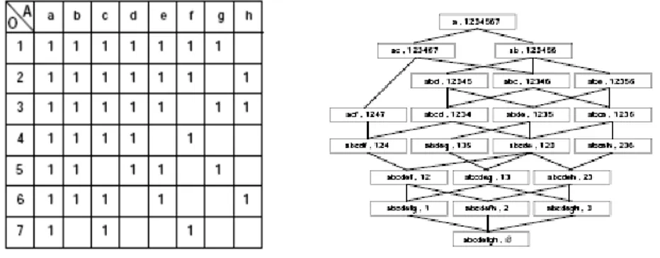
For instance, the objects may be the students for some diploma. A property may be the final “pass” grade at a course, Fig. 1. A closed set would be any couple (S, P) such that S contains all the students who passed all the courses in P, and, for any other course, at least one of the students in S failed. It could be for example students 1,3,5 who were the only and all to pass courses a,b,d,e,g. The Galois lattice would show the inclusion connections. It could show for instance for our closed set that students 1,3 form also a close set over more courses as they share also d. The set of students pass-ing all the exams (one extremity of the lattice) may or may not be empty. Likewise, there may or may not be the course that all students pass (the other extremity). The dean may obviously be interested in mining the resulting (Galois) connections, i.e.,

searching for some closed sets or selected parts of the lattice. Obviously if a close set includes many more students and much fewer courses than any other, these courses are perhaps a little too easy.

There were interesting applications of the concept analysis to databases, e.g., to mine for ISA relationship, [12]. Our example shows however also that the theory of Galois connections over binary attributes is intrinsically of limited value for that field. After all, courses usually have multi-valued grades, e.g., 0 to 20 in Dauphine. It is a truism to say that relational databases deal almost exclusively with multi-valued at-tributes. If the concept analysis should apply to databases at a larger scale, there is a need for the related generalization of its universe of discourse. The need may obvi-ously concern applications to other domains. The latter triggered already two gener-alization attempts, [4], [11], and a trend called scaling that instead attempt to map the multi-valued attributes into binary ones. All these proposals were not specific to data-bases and, as we show later, were in fact too limited for our goal. For instance, the scaling would typically require a change to the database schema under consideration. The proposals in [4] would be limited to attributes with totally ordered domain, and, even in this case, would present other important limitations. Like [11],although for other reasons.

We therefore propose a different generalization, tailored specially for the database needs. As the result, we may mine for the Galois connections using SQL. We mine for the closed sets especially, through a perhaps surprising relationship to the concept of a grouping in SQL queries through the popular GROUP BY, CUBE etc. operators. As the result, we propose a generalization of these operators and a new aggregate function. The database mining gains then new kinds of queries inherited from the work on the concept analysis, which are hard or impossible to achieve with SQL at present. In turn, the concept analysis inherits the database techniques for mining large collections of data. These should help that domain, whose algorithms are basically limited in practice at present to relatively small collections only, i.e., dozens of ob-jects usually and hundreds at most.

To give an idea of our proposal, observe that the notion of sharing a multi-valued property may be given various meanings. Observe further that the basic operation in the relational database universe of discourse, that is an equi-join, may be meant as a property sharing. The meaning is that the values of the join attributes are equal through the “=” comparison operator. More generally, the sharing may concern any operator in the set θ = {=, ≤, <, <>, ≥, > }. This is the idea in the θ-joins. The mean-ing of “≤” operator for instance is that an object with a property symbolized by a join attribute value v, shares this property with any other object whose value v’ of the join attribute is such that v ≤ v’. Joins seen under this angle are also some Galois connec-tions. Notice in particular, in the light of the comments to [4] above, that the use of operators “=” and “<>” does not require a total order on the domain of the join attrib-utes.

Next, observe that the popular GROUP BY operator, also explores the ‘=’ Galois connection among the objects (tuples) that it groups over the given set of (grouping) attributes. More generally, the popular CUBE operator groups over any subset of the set of the grouping attributes, but also along the same ‘=’ connection, [8]. A group T over some of the attributes under the CUBE, together with every other column form-ing a group over some other attributes of the tuples in T, if there are any such

col-umns, form a closed set in this sense. Hence, CUBE is the basis for some closed sets computation and analysis. Subsequently, one may order the closed sets by inclusion, getting a generalized Galois lattice.

The generalization of the grouping operators we propose below follows this ap-proach. In short, the new operators group for the other θ-operators as well. We may then calculate the closed sets also over the other θ values. The idea is somehow simi-lar to that in θ-joins with respect to the ‘=’-join (equi-join). The new operator general-izing the CUBE for instance, groups as CUBE, but over the other θ values as well, even different ones combined in a single grouping operation. We term it T-CUBE and read θ-CUBE. It. We act similarly with respect to GROUP BY, ROLLUP and GROUPING SETS, proposing the T-GROUP BY etc. The Galois lattices can be fur-ther formed by inclusion over the closed sets.

Like CUBE, T-CUBE does not show explicitly the tuples it has grouped to form a closed set. We combine for this purpose the operator with the LIST aggregate tion [14]. To show the attributes of the closed set, we propose a new aggregate func-tion we call T-GROUP. The funcfunc-tion renders an aggregated value at an attribute iff given tuples form a group at that attribute over given θ. Otherwise, the result of T-GROUP is null. As typically for the databases, we can further combine the mining of a closed set with that of the attributes not in the set. We can apply any SQL aggregate function to these attributes. Likewise, we can apply aggregate functions other than T-GROUP to the attributes forming the closed sets.

One knows well that CUBE operator is hard to evaluate. The evaluation of T-CUBE may be obviously be even harder. A variety of algorithms for T-CUBE have been proposed and could serve for ‘=’ closed sets calculus. We propose below algo-rithms applying also to the other θ ‘s. They use the scalable distributed calculus of P2P or grid type that appears the most practical. One algorithm uses a distributed hash scheme valid for all θ’s. Another scheme we termed SD-ELL is specific to θ = ’≥’

Below we recall the formal definitions of the closed sets and of Galois lattices. Next we define the syntax and semantics of T-CUBE. Finally, we discuss the compu-tation of our closed sets. We conclude with the direction for the future work.

2. Galois

Connections

The Galois connections are the mathematical framework for extracting concepts and rules from other concepts. The closed sets and the Galois lattices are the most studied connections. To recall the basics, a formal context is a triplet (O,A,I), where O is a set of objects, A is a set of attributes, and I is a binary relation between A and O (I⊆O×A). The notation o I a, o∈O, a ∈A, indicates that (o,a) ∈ I. For O1⊆O, let O1’ be the set of the common attributes to all these objects, i.e., O1’= {a∈A | o I a for each o∈O1}. Vice versa, for A1⊆A, let A1’ be all the objects verifying all the attributes of A1, i.e.,A1’= {o∈O | o I a for each a∈A1}. A Galois connection (GC) is the pair of mappings that we denote (f, g), over P(O) and P(A), where: f: O1→O1’ and g: A1→A1’. The couple (O1, A1) where O1 = A1’ and A1 = O1’ constitutes a closed set, (CS), also called concept. The set O1 (vs. A1) is called extent (vs. intent) of (O1, A1).

Fig. 1. A formal context C and its Galois lattice

We usually represent an object o as a tuple with an OID attribute and the binary at-tributes a that evaluate to .true or ‘1’ iff (o I a). Thus a = 1 means that o possesses the property represented by a. Fig.1 is an example of a formal context represented in this way, with O = (1,2,3,4,5,6,7) , e.g. students and A = (a,b,c,d,e,f,g,h), e.g., exams.

The (double) inclusion relation we denote as “≤ “ defines furthermore a partial order of all the concepts over a formal context:

(O1,A1) ≤ (O2,A2) ⇔ O1⊆O2 and A1⊇A2 ⇔ (O1, A1) is a subconcept of (O2,A2) ⇔ (O2, A2) is a superconcept of (O1,A1).

A sub-concept corresponds thus to a concept specialization, with possibly less ob-jects, but with possibly more .true attributes in common (common properties). A su-per-concept corresponds to the opposite, i.e., realizes an abstraction of its sub-concepts. A Galois lattice (GL) is finally the set of all the concepts, ordered by the re-lation ≤. Fig.2 shows the GL over the formal context at Fig. 1. Notice that we repre-sent the sub-concepts above the super-concepts. Several algorithms determine the CSs, or a GL over a formal context [7] [10]. In practice, these algorithms work only for contexts of a few hundreds of objects at most, i.e., small from the database mining perspective.

3

Multi-Valued Galois Connections

A relational database contains tuples whose attribute domains are typically multi-valued. This makes the notion of a GC and the related apparatus of the concept analy-sis theory basically inappropriate for the database management. The starting point of any application of these notions to the databases has to be some generalization to the multi-valued domain. We proceed towards this goal as follows. First, our objects of interest are the (relational) tuples We further define property sharing as follows. As we mentioned, the concept of a θ-join already provides some meaning of such sharing for the join attributes. We consider further a grouping operator θ, θ ∈ {=, ≤, <, <>, ≥, >}. Let a (t) be an attribute value of tuple t. Then, given θ, a set T of tuples t share the property defined by one or more following attribute values c:

Accordingly, consider that we choose c and θ at some attribute x. We say that T forms a θ-group for c at x, if every t in T shares c value according to the above rules. In the vocabulary of θ - joins, a tuple t belongs to a group formed at x iff t.x θ c =.true. We then call c a common property of group T. As usual, one can define the grouping at several attributes, as the intersection of the groups at each attribute chosen.

Given for each x a choice of θ and of some c, present in some tuple, we say that T and some set A’ of its attributes form a θ-closed set (T, A’) if T contains all and only tuples forming the groups for each attribute in A’, and there is no group involving all the tuples of T on an attribute not in A’. We abbreviate the term generalized closed set to θ-CS. The notions of a valued θ-Galois connection (θ-GC) and of a multi-valued θ-Galois lattice (θ-GL) define accordingly.

The choice of c for defining a θ-group and a θ-CS can be the usual one for θ = ‘=’. For the other θ values, we generalize the usual rule. Let some tuple s, termed seed, be in the table subject to the grouping. Let s.x be the value of attribute x of s. Let T be the group formed using some θ values at some attributes of s. Let θ (x) denote θ used at attribute x. Then, if s.x defines a group for θ (x) over tuples in T, we set c = s.x. We form A’ from all the groups formed in this way over s.

We represent (T, A’) for a relational calculus basically as a tuple t = (T, v(A)), where for each attribute x ∈ A’, t.x = c otherwise t.x is null what we denote as t.x = ‘_’. We qualify this representation of a θ-CS as basic. Observe that our rule for v (A) defines in fact a specific aggregate function, in the common, relational database, sense. We consider therefore also the aggregate representations of a θ-CS, where one forms t.x using a different aggregate function.

Example 1.We now illustrate our notions of θ - groups and of θ-CS, and their in-terest for the database mining. Hence, consider Table 1, tabulating relation S of stu-dents at Dauphine with key S#, and with the grades per course a,b…h. We wish to find any students with the grades of Student 1 for course a. If so, we wish to mine for the courses where these students also share the respective grade student 1.

The θ = ‘=’ at all the attributes of S answers our query. Students {1, 2} form then the group at a sharing c = 12. They form also the groups at f, for c = 13. The couple ({1, 2}, {a = 12, f = 13}) forms ‘=’-CS, responding to our query. We aggregate this θ-CS to the tuple ({1, 2},12,_ ,_,_,_,12,_,_}) compatible with the original table and be-ing the basic representation of the CS.

It should be seen that no current SQL dialect expresses the discussed query. Notice also that the calculus would apply to the single-valued attributes, e.g., to pas an exam for a student. It would lead to the usual CSs.

The similar query, but for any student and any course produces several θ-CSs : ({1,2,4,6}, {f = 13}), ({1,3,4}, {g = 12}), ({4, 6}, {b = 14, f = 13}), ({1, 4}, {d = 10, f = 13, g=12})…

We now mine for every student at least as good as student 1 for course a, and per-haps for other courses that we wish to mine therefore as well. We apply θ = ‘≥’ at all the columns, perform the grouping on column a, for a = 12, and find the groupings at other columns. We get the following θ-CS:

Table 1. Table S

Next, we wish the least grade of these students for every course, i.e., the minimal competence level they share. We use at each column the aggregate function c = minT (x), where T denotes the students in the group of student 1 over a. Our result is

now:

({1, 2,4,5},12,10 ,6,10,11,10,11,6}).

The result meets the definition of a CS over multi-valued attributes proposed in [4], termed a generalized CS. The example illustrates that the definition in [4] is a specific case of ours, limited to a ‘≥’-CS, in our vocabulary.

Yet alternatively, for our group {1,2,4,5}, and column b for instance, one could mine for avg (b). The result b = 13 would give a different measure of the difference between the grade of student 1 and of the other students for this course. Likewise, we may ask for students who are at least as good as any other student for any set of courses. The set of all ‘≥’-CSs will be the answer. In this example its cardinal is in fact 39. The calculus for the actual course, with about 20 students, showed over 6.000 θ-CSs. This hints about the difficulties for the efficient processing.

Next, we may have interest in the students at most as good as student 1 on a and possibly at some others courses, or better etc., [15]. We would use θ = ‘≤’ or θ = ‘>’at all columns getting, in the latter case, CS= ({4,5},12,_, _,_,12, _,_,_}). Again, no current SQL dialect would express the discussed queries.

4. T-CUBES

The notion of grouping is popular with the database management since the introduc-tion of GROUP BY operator. It calculates a single grouping over some columns. It uses Θ = ‘=’ in our vocabulary. Operators for multiple groupings followed. Among them, CUBE is the most general at present. We recall that CUBE (a1…an) calculates all the groups over all the subsets of {a1…an} for Θ = ‘=’ in our vocabulary. The CUBE appears as the natural basis for the calculus of θ-GCs in general, and of θ-CSs specifically. Notice that the notion of θ-CS appears as a natural 2-d extension of that of a group. It operates indeed not only on the tuples common to the group, but also on the common properties.

For our purpose, one has to first generalize CUBE operator so to accept the other values of θ as the grouping criteria. Next, one has to accompany it with aggregate

S# A b c d e f g h 1 12 16 6 10 12 13 12 6 2 12 12 8 12 11 13 11 8 3 10 13 16 14 11 8 12 10 4 13 14 11 10 13 13 12 14 5 17 10 10 14 13 10 14 12 6 0 14 3 8 4 13 11 10

functions that show the θ-CS composition, with respect to both the tuples and the at-tribute values. Notice that CUBE by itself does not provide the group composition at present. Our proposal is as follows.

We consider a new operator we call T-CUBE. The operator allows for any θ at any of the columns it should operate upon. It performs the multiple groupings accord-ingly, e.g., those in Example 1. For θ = ‘=’, T-CUBE reduces to CUBE. Over the groups provided by T-CUBE, we use basically two following aggregate functions to form the θ-CS tuple:

1. The LIST (I) function, [14], where I indicates the attribute(s) chosen to identify each tuple composing the θ-CS.

2. The T-GROUP (θ, x) function. This function tests whether column x forms a group, given a seed. If so, it renders c as the result, otherwise it evaluates to ‘_’. In the latter case, it may invoke another aggregate on the column.

For convenience, we consider T-GROUP (x) = T-GROUP (=, x). We also consider T-GROUP implicit for every attribute without a value expression named in the Select clause and T-CUBE. T-GROUP inherits then for each attribute its θ under T-CUBE. The function is also implicit for attributes without a value expression and not in the T-CUBE, provided T-CUBE uses only one θ value for all the grouping attributes.

We further consider that T-CUBE allows for a restriction on attributes X that is en-forced only when X are processed as the grouping attributes. For instance, in our mo-tivating example, one may indicate that, for query Q, only the values of a above 0 are of interest for θ = ‘≥’ groups to form at this attribute. When T-CUBE evaluation in Q leads in turn to the grouping on attribute b only, again just for instance, then Q con-cerns potentially all the values of a. Hence, we may a get a θ-CS involving student 6 with 0 grade.

Finally, as we allow for θ ≠ ‘=’ in T-CUBE, we implicitly generalize the GROUP BY, ROLLUP… to, respectively, T-GROUP BY, T- ROLLUP... clauses.

- Example 2. T-CUBE (a,b,c) means CUBE (a,b,c). Next, T-CUBE (≥,a,b,c) means the groupings using θ = ‘≥’ at all three attributes. To the contrary, T-CUBE (≥a, =b, >c) means the groupings using the different θ values at each attribute. Finally, T-CUBE (=,a : a <> 0,b,c) limits the interest to groups formed at a only for a not 0.

Next, the following query produces mining (1) requested in Example 1. The func-tion T-CUBE is implicit at attributes a…h.

Select List (s#),a,b,c,d,e,f,g,h from S

T-CUBE (a)

having a = (select a from S where s# = 1)

Here the functions T-GROUP (=, a)… are implicit. We could write the query alterna-tively in many ways, [15]:

The next easy query also follows up on Example 1. It gets the generalized CS of [4], adds to it the average values for b at each group, and restricts the mining to CSs formed from at least 2 members.

Select List (s#), min (a), min (b), min (c), min (d), min (e), min (f), min (g), min (h), avg(b)

T-CUBE (≥, a,b,c,d,e,f,g,h) having count(*) > 1;

See [15] for more motivating examples.

5. T-CUBE

Evaluation

The CUBE possibly generates many and big groups [8]. T-CUBE may obviously gen-erate even larger groups. Efficient algorithms for T-CUBE queries are therefore cru-cial. Besides, with respect to our aggregate functions, the single-attribute LIST func-tion, limited in this way with respect to its semantics in [14], but sufficient here, is standard at SQL Anywhere Studio. This DBMS does not however offer CUBE. Ten-tative implementations of single-attribute LIST as user-defined functions were also at-tempted under Oracle that has CUBE. In turn, we are not aware of any implementa-tion of GROUP funcimplementa-tion as yet. Fortunately, one may expect the task of creating T-GROUP as a user-defined function rather simple. These are already in the commercial word, e.g., Oracle and DB2. SQL Server should get user-defined functions in the next release. DB2 and SQL Server have CUBE

With respect to T-CUBE evaluation a scalable distributed architecture for grid or P2P environment seems the best basis at present, [15]. We consider that the dis-patcher node (peer) coordinates the query evaluation. It calculates any restrictions, and distributes, possibly uniformly, the remaining calculus of θ-CSs to the P2P appli-cation nodes. Only one node possibly determines a θ-CS. The number of nodes in-volved is chosen so that each one has a reasonably small and about the same number of θ-CSs to find. A Scalable Distributed Data Structure (SDDS) , e.g. an LH* file, [13], stores the (distributed) result, possibly in the distributed RAM, for orders of magnitude faster access than to disks. Each θ-CS has a key, unique regardless of, per-haps, its duplicate production by different nodes. A duplicated θ-CSs if any, is disre-garded in this way when the node calls its local SDDS client component with. Each node reports to the dispatcher once it terminates. The dispatcher performs any post-processing or returns the control to the user.

To design the algorithms, one may start either from the database heritage or from the formal concept analysis heritage. The former approach implies the reuse of GROUP BY and CUBE algorithms, of some of a general relational query evaluation, and of some for an SDDS. The was a large body of work in these domains, [9], [8], [16]. The latter direction implies the algorithms already proposed for computing bi-nary CSs, [10]. More specifically, it involves the algorithms for generalized CSs, [4], [5]. We now examine both directions

5.1 Database Heritage

We target a general algorithm, applying to every θ. Algorithms valid for some θ only, θ = ‘=’ especially, are thus out of scope here. Notice however, as we mentioned, that the major DBMSs have already the CUBE operator, making the implementation of

‘=’-CS calculus potentially simpler. As for θ-joins, we consider some nested-loop ap-proach. The grouping calculus (i) visits thus sequentially all the tuples concerned, and (ii) for each tuple, it examines all the possible subsets of the attribute values. For each choice, termed the current seed, it visits other tuples in T, perhaps all, to determine the existing groups.

For instance, if we start with student 1, the successive seeds could be (12,_ ,_,_,_,_,_,_}), (_,16 ,_,_,_,_,_,_}), (12,16 ,_,_,_,_,_,_}), (_,_ ,6 ,_,_,_,_,_}), (12,_,6 ,_,_,_,_,_})… The 1st _{seed means the grouping calculus over a = 12. Next seed leads} to the grouping over a = 12 and b = 16 etc. Different seeds may produce different θ-CSs. They may alternatively produce a duplicate. The latter case results for instance from (12,_ ,_,_,_,_,_,_}) and of (_,_ ,_,_,_,13,_,_).

Our SD calculus replicates T on N > 1 nodes, numbered 0,1…N-1. The choice of N should let each node to compute θ-CSs only for a fraction of all the seeds. The subse-quent determination of N may be centralized or distributed. The former defines N up-front, given the estimate of the number of seeds to process and perhaps of θ-CSs wished to calculate per node. The latter lets the nodes to determine N dynamically.

We hint here about the centralized distribution only, see [15] for more. We form the seed as a large integer s concatenating the grouping attributes. Each application node generates the seeds or gets them pre-computed in a file, to avoid the duplicates. Then, all nodes use the same hash function h, mapping s on some number a = 0,1…N-1, where N is a parameter of h. Node a calculates then the θ-CS only for s such that h (s) = a. The dispatcher chooses N so to divide enough the interval [0, max(s)], where max(s) is the actual or a maximal possible s, e.g., with all the bits equal to 1. Each node attempts to store each θ-CS computed, with its key and all the aggregated values into SDDS, through its client. The key is the value of θ-CS also seen as inte-ger. This eliminates the duplicates, if any, as we have indicated.

5.2 Concept Analysis Heritage

Several algorithms for CS and GL calculus for binary attributes exist, e.g. the Ganter’s classic, [7]. As we mentioned, the universe of discourse of these algorithms makes them unfit for our database mining purpose. Most calculate a GL that is the is-sue we do not address here (yet). Whether some algorithms can be generalized to our goal remains an open issue.

The concept analysis community has of course noticed the multi-valued attributes. However the main direction to formally deal with, called scaling, was apparently simply to conceptually map such attributes into the binary ones, [11]. The scaling also seems unfit for our purpose. An alternative and exclusively formal approach to multi-valued GLs was suggested in [11]. It starts with a generic concept of description. This one assigns to an object set-valued attribute values, in the way somehow similar to the way proposed by the symbolic objects approach, [3]. It then orders the objects into a GL according to the inclusion of the descriptions (called precision of the descriptions) Our definition of GCs on the basis of the values of the θ-operator is “orthogonal” to the formalism of [11]. That formalism will be perhaps of more use for the databases if the set-oriented attributes become more popular.

Another generalization attempt, we already somehow discussed, apparently unknown to [11], is that in [4], together with the subsequent algorithms in [5]. In our approach, these proposals are all limited to the ‘≥’-CSs. In contrast, [4] mentions generalization directions we do not deal with, e.g., towards the fuzzy sets. Next, the proposed algo-rithms are not designed for the groupings with restrictions. They generate the full sets of ‘≥’-CSs. Already for quite a few tuples and attributes, these sets are in millions of CSs, [15].

Among these algorithms, one termed ELL, generating the ‘≥’-CSs only, i.e., with-out their GL, appears the fastest, [2]. ELL has two formulations, termed respectively iterative and recursive. A scalable distributed version of the iterative ELL was pro-posed in [1]. The idea was to partition the set of object or of attributes over the appli-cation sites. Unfortunately, as we have found, the calculus needed then the inter-application node communication, close to gossiping for every CS generated. The mes-saging cost of the algorithm was consequently prohibitive, already for even dozens of objects only.

In the wake of the study to overcome this limitation, the recursive ELL appeared an alternate basis for the scalable distributed computation. The “key to the success” was to replicate T1_{. This, - to offset the trouble in [1] that appeared largely due to the} partitioning of T instead. We have termed the new algorithm SD-ELL. Like the cen-tralized recursive ELL, SD-ELL recursively splits the computation C of the set of the CSs over T into more and smaller computations of subsets. It then distributes the com-putations with the copies of T on the application nodes. In the nut-shell, the SD-ELL dispatcher first picks up any tuple, let us say Student 1 in our Table S. It then splits C into C1 that calculates all the CSs that contain 1, and C~1 that does the opposite. C1 in-volves in particular the calculus of the CS, let it be A1, generated by 1, i.e., containing all and only tuples sharing all the values in 1. Technically, A1 contains thus all and only the tuples with the attribute values greater or equal to those in 1. The dispatcher calculates A1 by itself. In our example, we have simply A1 = {1}.

If only two nodes are available, i.e., N = 2, then the dispatcher sends the replicated T and the requests to perform the respective computations to these nodes. Each node uses then locally a slightly modified version of the interactive ELL. The nodes collect the calculated CSs in a (common) SDDS file. With luck, the CPU load of each node is about ½ of a single node. If it is too much or there are more volunteering nodes, the dispatcher decomposes the tasks further. To decompose C1, the dispatcher picks up any element in the set T/A1. This set contains all the tuples that can lead to a CS con-taining 1. Those in A1 other than 1 obviously cannot.

The dispatcher could pick up thus Student 2. C1 partitions then recursively into (i) task C1,2 computing all the CSs that contain both 1 and 2, and (ii) task C1,~2 that con-tains CSs with 1 alone. Each task goes to an application node, again along with the replicated T. Now, with the uniform distribution luck, both task may end up calculat-ing about ½ of the CSs devoted to C1. There is also again the CS, let us call it A1,2 that the dispatcher may calculate by itself. A1,2 contains all the tuples sharing the properties common to both 1 and 2. Actually, A1,2 = {1,2,4}.

On the C~1 task side, the dispatcher can first determine the actual set of tuples that cannot generate a CS with 1. This set, let it be R1, has to have all the tuples with the

attribute values that are at most equal to the respective ones in 1. Actually we have R1 = {1}. The dispatcher may further decompose C~1 as above, except that it uses R1 instead of A1. That is, it first picks up any element in the set T/R1, let us say 2 again. Then it defines the tasks C~1,2 calculating all the CSs that contain 2, but not 1, and its “sibling” C~1,~2 that contains neither tuple. The tasks can be sent to two nodes, again along with T.

The replication of T results from a subtlety of the above dichotomies. The calculus of CSs may lead to a kind of collisions for SD-ELL, although not the same as for the hashing calculus. The collision may concern a task that should not include a tuple, e.g., C1,~2 with its sibling, C1,2 here. A set generated at the former, intended as a CS, may happen to be in fact only a strict subset of a CS at the latter, hence not a CS at all in fact. The difference may be a tuple to avoid at the former, student 2 here. Any CS involving this tuple should be, and effectively is, generated by the sibling, by its defi-nition itself. The task generating the subset should therefore be able to recognize the collision locally. It can, by testing, for each generated set, each tuple to avoid speci-fied in the task definition, e.g., 2 in our case. The test should show that the attribute values of the tuple do not share the common properties of the set. We recall that these are the minimal value of each attribute over the set. Having a copy of T, let every node to know locally any such values. Iff the test fails, the node recognizes the colli-sion and drops the set.

In our example for instance, C1,~2 generates the set {1,3,4,5,6}. The properties shared by all the elements of the set are (0,10,3,8,4,8,11,6). The result is not a CS. Student 2 indeed also shares these properties. Hence, 2 must belong to the resulting CS, involving thus the set {1,2,3,4,5,6}. However, task C1,2, by its definition, already calculates every CS involving 2. Hence, set {1,3,4,5,6} at the node with C1,~2 is a col-lision. The node of C1,~2 identifies the fact by the local test of the attribute values of 2, using its copy of T.As the result, it drops the set {1,3,4,5,6}.

All together, provided again the uniform distribution of the values, the 2nd _{level of} decomposition of both C1 and C~1 on four nodes, reduces the calculus time to about ¼ of that on a single-node. The dispatcher can continue to decompose each task recur-sively. Each decomposition reduces the remaining set of tuples, after chopping off the next A or R. Hence, the dispatcher can decompose and possibly reduce the overall execution time, as long as (i) the remaining set of tuples is not empty, and/or (ii) there are spare P2P nodes. One can possibly run into thousands of nodes. A P2P or grid net, seems in this way the only way towards the practical response time for a larger T, characteristic of the database mining.

The SD application of ELL (SD-ELL) appears a potential basis for ‘≥’-CSs calcu-lus, with respect to both the distribution and the calculus schemes. Provided however that one can re-engineer it for the restrictions. See [15] for more on SD-ELL.

6. Conclusion

T-CUBE operator, coupled with the LIST and T-GROUP aggregate functions, ap-pears useful for data mining. through the multi-valued Galois connection analysis in larger collections. The P2P and grid environment appears the most appropriate

im-plementation support. Known algorithms for the CUBE processing may apply to T-CUBE for specific θ values.

Future work should concern deeper analysis and implementation of the described T-CUBE evaluation algorithms. One should also implement the multi-attribute LIST and T-GROUP functions The processing of the (multi-valued) θ-GLs remains to be studied. It seems related to lattices in [6]. Finally, the operators GROUP BY, T-ROLL UP, T-GROUPING SETS should be studied on their own.

Acknowledgments. A grant from Microsoft Research partly supported this research. The

European Commission project ICONS no. IST-2001-32429 helped with early work towards SD- ELL.

References

1. Baklouti. F, Lévy. G. Parallel algorithms for general Galois lattices building. WDAS 2003, Carleton Scientific (publ.).

2. Baklouti. F, Lévy. G. A fast and general algorithm for Galois lattices building. Submited to the Journal of Symbolic Data Analysis. April 2005, 1st _revision.

3 Diday, E. Knowledge discovery from symbolic data and the SODAS software. The 4th Eu-rop. Conf. onPrinciples and Practice of KnowledgeDiscovery in Databases, PPKDD-2000. Springer (publ.).

4. Diday. E, Emilion. R. Treillis de Galois maximaux et capacités de Choquet. Cahier de Re-cherche de l’Acadèmie des Sciences. Paris, t.325, Série I, p.261-266, 1997.

5. Emilion. R., Lambert. G, Lévy. G, Algorithmes pour les treillis de Galois. Indo-French Workshop., University Paris IX-Dauphine. 1997.

6. Fagin, R. & al. Multi-Structural Databases. Intl. ACM Conf. on Principles of Database Sys-tems. ACM-PODS 2005.

7. Ganter. B. Two basic algorithms in concept analysis. Preprint 831, Technische Hochschule Darmstadt 1984.

8. Gray, J & al. Data Cube: A Relational Aggregation Operator Generalizing Group-By, Cross-Tab, and Sub-Totals. Data Mining and Knowledge Discovery J.,1 , 1, 97, 29 – 53. 9. Garcia-Molina, H., Ullman, J., Widom, J. Database Systems: The Complete Book. Prentice

Hall, 2002.

10. Ganter, B. Wille, R., Franzke, C. Formal Concept Analysis: Mathematical Foundations. Springer-Verlag New York, 1999, 294.

11. Gugisch, R. Many-valued Context Analysis using Descriptions. H. Delugach and G. Stum-me (Eds.): ICCS 2001, LNAI 2120, 157-168, 2001, Springer-Verlag.

12. Hainaut, J-L. Recovering ISA Structures. Introduction to Database Reverse Engineering. Chapter 14. (book in preparation), 2005.

13. Litwin, W., Neimat, M.-A., Schneider, D. LH* : A Scalable Distributed Data Structure. ACM Transactions on Database Systems (ACM-TODS), 12,.96.

14. Litwin, W. Explicit and Implicit List Aggregate Function for Relational Databases. IASTED Intl. Conf. On Databases and Applications, 2003.

15. Litwin, W. Galois Connections, T-CUBES, & P2P Database Mining. 3rd Intl. Workshop on Databases, Information Systems and Peer-to-Peer Computing. VLDB 2005. Also CERIA Res. Rep. 2005-05-15, May 2005

[16] Litwin, W. Scalable Distributed Data Structures. ACM 13th _{Conf. On Inf. and Knowledge} Mangment (CIKM-2004), Washington DC. 3h Tutorial.