Waterpixels et Leur Application à l'Apprentissage Statistique de la Segmentation

HAL Id: tel-01537814

https://pastel.archives-ouvertes.fr/tel-01537814v2

HAL is a multi-disciplinary open access archive for the deposit and dissemination of sci-entific research documents, whether they are pub-lished or not. The documents may come from teaching and research institutions in France or abroad, or from public or private research centers.

L’archive ouverte pluridisciplinaire HAL, est destinée au dépôt et à la diffusion de documents scientifiques de niveau recherche, publiés ou non, émanant des établissements d’enseignement et de recherche français ou étrangers, des laboratoires publics ou privés.

Vaïa Machairas

To cite this version:

Vaïa Machairas. Waterpixels et Leur Application à l’Apprentissage Statistique de la Segmentation. Traitement du signal et de l’image [eess.SP]. PSL Research University, 2016. Français. �NNT : 2016PSLEM099�. �tel-01537814v2�

de l’Université de recherche Paris Sciences et Lettres

PSL Research University

Préparée à MINES ParisTech

WATERPIXELS AND THEIR APPLICATION

TO IMAGE SEGMENTATION LEARNING

École doctorale n

432

SCIENCES DES MÉTIERS DE L’INGÉNIEUR

Spécialité

Soutenue par

Vaïa MACHAIRAS

le 16 Décembre 2016

Dirigée par

Etienne DECENCIÈRE

et Thomas WALTER

COMPOSITION DU JURY :

Mr Nicolas PASSAT

Université de Reims Champagne-Ardenne Président

Mme Corinne VACHIER Université Paris Est Créteil Rapporteur

Mme Thérèse BALDEWECK L’Oréal Recherche et Innovation Membre du jury

Mme Valery NARANJO

Universidad Politécnica de Valencia Membre du jury

Mr Jean SERRA

ESIEE, Membre du jury Mr Etienne DECENCIÈRE

MINES ParisTech, Membre du jury Mr Thomas WALTER

Remerciements

Cette thèse a été réalisée au Centre de Morphologie Mathématique (CMM), sur le site de Fontaine-bleau de MINES ParisTech. Je tiens à remercier mes deux encadrants, Etienne Decencière (CMM) et Thomas Walter (Centre de Bio-Informatique de l’Ecole) pour leur aide et leur confiance tout au long de ces trois années. Leur implication, leur soutien et leurs conseils avisés m’ont permis de beaucoup progresser et d’avoir toujours envie de me dépasser.

Je souhaiterais remercier les membres de mon jury, Mr Nicolas Passat (président du jury et rap-porteur), Mme Corinne Vachier-Lagorre (raprap-porteur), Mme Thérèse Baldeweck (examinatrice), Mme Valery Naranjo (examinatrice) et Mr Jean Serra (examinateur), pour leur intérêt pour les waterpixels et de m’avoir permis d’obtenir le titre de Docteur en Morphologie Mathématique.

Pour qu’un enfant grandisse, il faut tout un village. (Proverbe africain)Cette thèse n’aurait pas été si épanouissante, tant d’un point de vue scientifique que personnel, sans la présence d’un grand nombre de personnes. J’ai eu la chance de pouvoir vivre cette belle expérience entourée par la grande famille du CMM. Je tiens donc à remercier Fernand Meyer et Michel Bilodeau de m’avoir accueillie pour mon stage puis ma thèse respectivement, et tous les collègues que j’ai pu rencontrés pendant ces deux périodes: Dominique Jeulin, Serge Beucher, Jesus Angulo, Beatriz Marcotegui, Petr Dokladal, Petr Matula, François Willot, Matthieu Faessel, Serge Koudoro, Bruno Figliuzzi, Santiago Velasco-Forero, mais aussi Julie, Hellen, Vincent, Thibaud, Xiwei, Torben, El Hadji, André, John, Dario, Andres, Bassam, Enguerrand, Emmanuel, Amira, Luc, Nicolas, Jia-Xin, Joris, Jean-Charles, Gianni, Haisheng, Sebastien, Amin, Jean-Baptiste, Théodore, Robin, Antoine, Kaiwen et Albane. Je n’oublierai pas les bons moments passés ensemble et toutes les discussions que nous avons eu pour refaire le monde (avec ou sans morphologie mathématique). Mention spéciale à mi hermanito, qui a été un modèle pour moi tout au long de ma thèse, et à la team de printemps/été/automne/hiver qui a toujours été là pour moi et qui a été exceptionnelle en toutes circonstances. Last but not least, rien n’aurait pu se faire sans la participation de Catherine Moysan et Anne-Marie De Castro, deux secrétaires en or, d’une générosité sans bornes.

Je souhaiterais aussi remercier les collègues rencontrés en dehors du CMM, notamment Gaëlle, Pascale, Laura, Claudie, Jihane, Emilie, Marine, Ricardo, Dariouche, Pierre, Nelson, Angélique, Arezki, Julia, Aurélie et Lydia. Votre amitié a été très précieuse. Merci également à toute la team du mardi, qui m’a suivie dans ce merveilleux projet avec confiance et enthousiasme. Vos sourires et votre détermination ont été pour moi la plus belle des récompenses.

Je tiens à remercier tous nos collaborateurs sur ce projet : Peter Naylor du CBIO, Nicolas Passat, Jimmy Francky Randrianasoa, Andrés Troya-Galvis, Pierre Gançarski en Alsace, David Cardenas Pena en Colombie, Thérèse Baldeweck de L’Oréal Recherche et Innovation; ainsi que nos collaborateurs lors de mon stage : Marie-Claire Schanne-Klein, Stéphane Bancelin, Carole Aimé, Thibaud Coradin et Claire Albert.

Merci à Sabine Süsstrunk, Kawalina, Flavien, Kaem et Marine, Céline et Cain, Carolina et Mehdi Kerkouche de m’avoir inspirée au cours de ces trois années. Merci aussi à Mme El Mejri, Mme Rivière, Mme Adams, Mme Turin, Mohammed, Mr Baume et Mr Hébert pour leurs

en-Enfin un immense merci à toute ma famille, en particulier à mes parents et ma soeur Lara qui ont toujours été là pour moi. Je vous aime.

Je terminerai avec deux citations utiles à tout doctorant préparant une thèse :

It always seems impossible until it’s done.Nelson Mandela.

a a

Résumé

L’objectif de ces travaux est de fournir une méthode de segmentation sémantique qui soit générale et automatique, c’est-à-dire une méthode qui puisse s’adapter par elle-même à tout type de base d’images, afin d’être utilisée directement par les non-experts en traitement d’image, comme les biologistes.

Pour cela, nous proposons d’utiliser la classification de pixel, une approche classique d’appren -tissage supervisé, où l’objectif est d’attribuer à chaque pixel l’étiquette de l’objet auquel il appar-tient. Les descripteurs des pixels à classer sont souvent calculés sur des supports fixes, par exemple une fenêtre centrée sur chaque pixel, ce qui conduit à des erreurs de classification, notamment au niveau des contours d’objets. Nous nous intéressons donc à un autre support, plus large que le pixel et s’adaptant au contenu de l’image : le superpixel.

Les superpixels sont des régions homogènes et régulières, issues d’une segmentation de bas niveau. Nous proposons une nouvelle façon de les générer grâce à la ligne de partage des eaux, les waterpixels, méthode rapide, performante et facile à prendre en main par l’utilisateur. Ces superpixels sont ensuite utilisés dans la chaîne de classification, soit à la place des pixels à classer, soit comme support pertinent pour calculer les descripteurs, appelés SAF (Superpixel-Adaptive Features). Cette seconde approche constitue une méthode générale de segmentation dont la perti-nence est évaluée qualitativement et quantitativement sur trois bases d’images provenant du milieu biomédical. a a *** a a

a a

Abstract

In this work, we would like to provide a general method for automatic semantic segmentation, which could adapt itself to any image database in order to be directly used by non-experts in im-age analysis (such as biologists).

To address this problem, we first propose to use pixel classification, a classic approach based on supervised learning, where the aim is to assign to each pixel the label of the object it belongs to. Features describing each pixel properties, and which are used to determine the class label, are often computed on a fixed-shape support (such as a centered window), which leads, in particular, to misclassifications on object contours. Therefore, we consider another support which is wider than the pixel itself and adapts to the image content: the superpixel.

Superpixels are homogeneous and rather regular regions resulting from a low-level segmen-tation. We propose a new superpixel generation method based on the watershed, the waterpixels, which are efficient, fast to compute and easy to handle by the user. They are then inserted in the classification pipeline, either in replacement of pixels to be classified, or as relevant supports to compute the features, called Superpixel-Adaptive Features (SAF). This second approach consti-tutes a general segmentation method whose pertinence is qualitatively and quantitatively evaluated on three databases from the biological field.

a a

***

a a

a a

List of the main abbreviations

MOMA Mathematical morphology SAF Superpixel-adaptive feature

SP Superpixel UC Unit of classification WP Waterpixel a a *** a a

Contents

1

1.1 Context and motivation 13 1.2 Thesis outline 15

I

Segmentation and Classification

2

2.1 General scheme for pixel classification 21 2.2 Features 22 2.2.1 Definitions . . . 23

2.2.2 Operators Ω and computational supports CS . . . 24

2.3 A powerful machine learning method: Random Forests 25 2.3.1 Principle and application to classification . . . 25

2.3.2 Settings . . . 28

2.4 Conclusion 29

3

3.1 Evaluation procedure 31 3.1.1 The L’Oréal databaseD1 . . . 32

3.1.2 The CAMELYON databaseD2 . . . 32

3.1.3 The Coelho databaseD3 . . . 35

3.3 Conclusion 44

II

Waterpixels

4

4.1 Definition and properties 57

4.2 Related work 58

4.2.1 State-of-the-art generation methods . . . 59 4.2.2 Superpixels and watershed . . . 61

4.3 Evaluation procedure to assess superpixel performance 61

5

5.1 Construction of Waterpixels 65

5.1.1 Selection of the markers . . . 66 5.1.2 Spatial regularization of the gradient and watershed . . . 72

5.2 Recap of the proposed method 73

5.3 Comparison with other watershed superpixels methods 73

5.4 Benchmark 74

5.4.1 Implementation details . . . 74 5.4.2 Results . . . 74 5.4.3 Computation time . . . 78

5.5 Conclusion, discussion and prospects 79

III

Learning Segmentation with Waterpixels

6

6.1 Examples of use in the literature 85

6.2 Superpixel classification 89

6.2.1 Principle . . . 89 6.2.2 Preliminary study onD1 . . . 90

6.3 Discussion and conclusion 96

7

7.1 Principle 103

7.2 Comparison with other state-of-the-art methods 104

7.3 Preliminary study onD1 106

7.3.1 Best achievable prediction with waterpixels . . . 106 7.3.2 Study with different families of features . . . 106

7.4.1 Presentation of the final results . . . 109 7.4.2 Discussion of the results . . . 112

7.5 Conclusion and prospects on SAF 121

7.5.1 Conclusion . . . 121 7.5.2 Prospects . . . 121

8

8.1 Conclusion 123

8.2 Prospects 124

A

Appendices

A.1 Optimization of Random Forest parameters 129

A.2 Mean mismatch factor definition 130

1

Introduction

Hope is a choice. Mary Margaret, Once Upon a Time.

Résumé

L’objectif de ces travaux est de fournir aux non-experts en analyse d’image une méthode générale de segmentation qui puisse s’appliquer facilement à toute base d’images sans avoir besoin d’être adaptée à chaque fois par l’utilisateur. Ce chapitre présente le sujet de thèse ainsi que le plan du manuscrit.

*****

1.1 Context and motivation

Object recognition is one of the most challenging tasks in image analysis. It is particularly useful in the biomedical field, for example, where progress in imaging techniques makes it possible to acquire more and more images with an increasing precision in order to help biologists in their analysis for instance. Processing this data (e.g. counting cells to compute the proportion of abnor-mal ones, tracking a specific structure through hundreds of slices of a 3D volume corresponding to the MRI of a brain, etc) turns out to be not only tedious (and a potential cause of errors) but also a waste of time in the elaboration of the diagnosis or in the scientific progress towards a better knowledge of biomedical phenomena. Therefore, images are more and more dealt with in an auto-matic way, in order to save time and ease biologists every day life. This is also true in many other fields, such as in security, urban scene understanding, remote sensing, or even social networks.

In this work, we focus on a special task of object recognition: semantic segmentation. Se-mantically segmenting an image consists in partitioning it into regions which have a meaning, i.e. which correspond to real objects in the scene. Each region of this resulting partition is defined by a set of pixels which have the same intensity value. This value, called label, corresponds to a unique class of objects (e.g. cars, cells, persons, . . . ).

mentations. The case of image 1 illustrates the search for the main object in the foreground (here a tree) in opposition to the background. Thus, the final segmentation presents only two labels. Figure 1.1.d presents a segmentation of nuclei of image 2, which are assigned the same label as they belong to the same class “nucleus”. Finally, the third case, image 3, emphasizes the fact that, for a given image, a segmentation is not unique as we may want to isolate different types of objects, leading each time to a different segmentation result. Figures 1.1.f and 1.1.g are two possible segmentations of image 3, targeting respectively all figures and only the eight. Therefore, the corresponding segmentation method must be designed to find the specified target. Moreover, due to the difficulty of creating such a method, commonly used segmentation tools are often opti-mized not only for a specific type of object but also to a specific type of images (imaging device, acquisition conditions, etc). Dealing with new images and new objects hence requires, most of the time, a different segmentation method to be designed, which takes time. It is worth noting that in most cases, images are to be dealt with not one by one but rather gathered into databases, i.e. sets of images sharing similar properties (same types of objects and/or same acquisition conditions etc). Unfortunately, due to the variety of objects and images to be analyzed, it also takes time to design for each database a specific segmentation method, as pointed out above.

(a) Image 1 a

(b) Segmentation of the main object in (a)

(c) Image 2 a (d) Segmentation of nuclei in (c) (e) Image 3 a (f) Segmentation of figures in (e) (g) Segmentation of eight in (e)

Figure 1.1: Segmentations of different images. Each segmentation presented here is a groundtruth, i.e. what we would like to obtain at the end of the segmentation procedure. Often per-formed manually, groundtruth is used as reference when evaluating quantitatively the performance of a segmentation method.

In this work, our aim is to provide a general segmentation method which could be easily ap-plied to any image database and by any user regardless of the latter’s potential (non-)knowledge of image analysis tools.

We will address this issue with a classification framework (supervised learning). Image pixels (or more precisely the vectors representing them) will constitute the data samples (at least in a first phase) and the classes will represent the different objects we would like to find in the image database. This approach requires that for each database, we already know the labels of some pixels to perform the training phase, i.e. we know to which objects some pixels belong. For this purpose,

we will use some images of the database which are already segmented by hand by the experts needing the segmentation of their database. The machine learning method we use will hence try to reproduce the best it can the way experts work when they visually analyze the content of their images.

Remark 1: Thanks to our collaborations, we will focus mainly on databases coming from the biomedical field (see Chap. 3). However, the proposed method is general and can be applied to any other databases.

Remark 2:The considered databases presented groundtruth with complete annotations (i.e. pixels were labeled), but only a set of examples for each object class would have been enough to perform the training phase.

1.2 Thesis outline

As we have seen, the aim of this work is to provide a general segmentation method achieving good performance on any image database without needing to be modified each time by the user (expert or not in image analysis), as far as the latter provides some examples already segmented by hand within the database to be segmented.

As previously announced, we first propose, inspired by the literature, to address this issue with pixel classification, a general approach based on supervised learning. Part I is dedicated to the set up and assessment of such a workflow. This method is indeed constituted of several steps, which are expounded in Chap. 2. We then evaluate qualitatively and quantitatively this pipeline on different databases to check if it achieves good segmentation results no matter what the asked segmentation task is (see Chap. 3). This leads us to consider the solutions which could improve this already promising method.

We subsequently focus on another image representation, superpixels, producing a special low-level segmentation of the image. As pointed out by an abundant literature, this structure seems to be a promising lead to improve segmentation performance when using the general framework of classification.

In Part II, we remind what superpixels are and which specific properties they should satisfy (see Chap. 4). With the help of another field of image analysis, namely Mathematical Morphol-ogy, we propose a new method to generate them based on the watershed transformation (see Chap. 5). We show that these superpixels, hence called waterpixels, offer good performance in terms of quality and computation time.

Once generated, these superpixels can be used to improve the classification pipeline performed to obtain the final segmentation. Part III presents two different uses of waterpixels in such a work-flow: superpixel classification (as proposed in the literature) and a novel application: Superpixel-Adapative Features (SAF). They are expounded in Chap. 6 and Chap. 7 respectively.

Conclusion and prospects are then presented in Chap. 8. a

tion of this PhD is to study the relevance of the image representation embodied by superpixels in the proposed workflow.

On another level, we also would like to show that Machine Learning and Mathematical Mor-phology are two powerful fields which can benefit from each other in order to go one step further towards efficient and automatic object recognition.

We have decided to make our codes available to the scientific community. They can be down-loaded on our website: http://cmm.ensmp.fr/∼machairas/. Programming was done in Python, with the help of Morph-M (seeKoudoro et al.[2012]), SMIL (seeFaessel and Bilodeau[2013]), scikit image (van der Walt et al.[2014]), numpy (Dubois et al.[1996],Ascher et al.[1999] and

Oliphant[2006]), mahotas (Coelho[2012]), scikit learn (Pedregosa et al.[2011a]) and Vigra li-braries (Köthe[2000]).

I

2

2.1 General scheme for pixel classification 2.2 Features

2.3 A powerful machine learning method: Random Forests

2.4 Conclusion

3

31

3.1 Evaluation procedure

3.2 Assessment of the pixel classification workflow on

Segmentation and

Classification

supervised learning.

In this part, we propose to address this issue with a classic approach often used in the liter-ature: pixel classification. Indeed, it consists in assigning to each pixel the label of the object type it belongs to. At the end of the process, all pixels which have obtained the same label form one or more connected components which belong to the same type of structures (e.g. cells, cars, background, . . . ). The result constitutes the semantic segmentation of the image.

If it is appropriately designed, this pipeline can perform supervised learning on every database, requiring only, from the user, to provide each time some examples of images already segmented by hand. This is why it is used by general segmentation software dedicated, for instance, to the biological field (such as Ilastik bySommer et al.[2011]).

In a first phase, we expound and set up such a workflow with general features (standard opera-tors used by Ilastik, operaopera-tors from mathematical morphology, textural features: Haralick and Ga-bor filters) and Random Forests (Breiman[2001]). We apply this pixel classification to three dif-ferent databases coming from the biological field (L’Oréal, CAMELYON16,Coelho et al.[2009]) and analyse the segmentation performance of this approach.

We conclude by suggesting to insert superpixels in this pipeline, a solution which is more thoroughly presented and assessed in Parts 2 and 3.

2

Segmentation as a classification

task

La philosophie est écrite dans ce grand livre qui s’étend chaque jour devant nos yeux : l’univers. Mais on ne peut le comprendre si nous n’apprenons d’abord son langage et si nous ne comprenons les symboles avec lesquels il est écrit. Galilée

Résumé

Dans ce chapitre, nous décrivons une approche classique de segmentation d’image qui utilise l’apprentissage statistique pour s’adapter à tous types de bases d’images. En ef-fet, le choix a été fait dans ces travaux de thèse de voir la segmentation comme une tâche de classification, où l’objectif est d’assigner à chaque pixel l’étiquette du type d’objet auquel il appartient. Nous exposons comment construire une chaîne de classi-fication de pixels en utilisant des descripteurs de pixels généraux issus de la littérature ainsi qu’une méthode d’apprentissage robuste et efficace : les forêts aléatoires (Breiman

[2001]). Cette chaîne sera évaluée qualitativement et quantitativement sur plusieurs bases d’images dans le chapitre suivant.

*****

In this work, we have decided to consider segmentation as a classification task, where the aim is to assign to each pixel the label of the object it belongs to. This chapter is dedicated to expound how pixel classification works (see Sec. 2.1), how we build this classic pipeline with elements from the literature (see Sec. 2.2 and Sec. 2.3) and why it enables to design a general segmentation method working on different databases.

2.1 General scheme for pixel classification

In this section, we will expound how pixel classification works on a given image databaseD. Note that this procedure should be performed every time the image database changes.

Recall that databaseD is split into two subsets: D_T (manual segmentations available) used for training phase andD_P(images to be segmented) used for prediction phase.

Figure 2.1: General scheme for pixel classification.

for example {0, . . . , 255} when f is an 8 bit grey level image or {0, . . . , 255}3 for color images. The aim is to assign to each pixel x ∈ D a label l(x) ∈C , where C = {c1, c2, . . . , cK} is the set

of labels corresponding to the K categories of objects to be found. The scope of this work will be limited to binary classification (i.e. C = {0,1}) but can easily be extended to more than two classes. At this stage, the two classes could be “object (1) vs. background (0)” or “contour of an object (1) vs. not an object contour (0)”. We will prefer here the region approach corresponding to the former. This also implies that the groundtruth should be provided in the same format.

The general scheme for pixel classification is illustrated in Fig. 2.1. Note that pixels constitute units of classification(UC), i.e. they are the elements to which we would like to assign a label at the end of the process. As a supervised learning technique, classification is comprised of two phases: a training step and a prediction step. The aim of training is to establish the classifica-tion rules assigning a label to each pixel. As explained in the previous chapter, this first phase is performed on the set of pixels ofD_T for which labels are already known since they are part of the images which have already been manually segmented by experts. The task of the learning method (notation: ML method) is to understand the link between this already known label and the pixel’s properties which are subsumed into its vector of features. Then, in the second phase, called prediction, any new pixel fromD_P can be assigned the label of the object it belongs to by computing its vector of features and giving the latter as input to the learning method which will apply the learned prediction function and find the pixel’s label.

Notation 2.1. If p is the number of features computed for a pixel x, then each vector v(x) is in Rp_.

We denote by X _{∈ R}n×p the data matrix which is given as input to the ML method for training, where n is the number of pixels inD_T.

In the following, we will get in more detail about the computation of the vector of features (see Sec. 2.2) and the machine learning method used (see Sec. 2.3).

2.2 Features

In this section, we will explain how to obtain the vector of features v(x) ∈ Rpof each pixel x used for training or prediction.

2.2.1 Definitions

First of all, what is a feature? A feature describes a pixel property. For instance, what is the inten-sity of the pixel? Or what is its position on the x-axis in the image? As an example, if the former is computed on a pixel of an 8-bit image, the answer will lie in the range [0, 255]. Note that the result may not be a number, e.g. when asking yes/no questions (Boolean) (e.g. is intensity greater than 140?), or if we get an histogram. In this work, all features used will be adapted so as to obtain a single value in R: yes/no can be converted to {0, 1}, an histogram with B bins can be converted to Bfeatures, etc. Indeed, this conversion step, easy to perform, is necessary as it is compulsory for the learning method used afterwards.

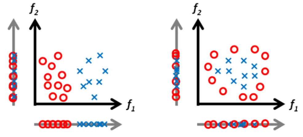
What is a “good” feature? A good feature is a feature that helps discriminate the data (here the pixels) into the two classes defined in the ground truth, as illustrated in Fig. 2.2.a, where each feature is represented by one dimension of the space: we can see that f1is a discriminant feature

(it is easy to find a threshold which can split perfectly the data into two pure groups), whereas f2

is not. Note that, even if a feature is not discriminant on its own, it can still be useful combined with others, as shown in Fig. 2.2.b. where the separation between the two classes must take into account the two features f1and f2to be efficient. In our case, we have decided to compute a large

number of general features (i.e. not specific to a given task) in order to ensure the generality of our method. Then, for each database, the power of discrimination of a given feature can vary, as well as for all their possible combinations. To ensure a good classification performance, we have chosen a machine learning method which is able, as far as possible, to discard “bad” features and use only “good” ones among the general set provided (see Sec. 2.3).

Figure 2.2: What is a good feature? More formally, a feature is defined as follows:

Definition 2.2.1 — Feature. A feature F can be described by the set of following elements:

F= {c, Ω, GEO,CS, Σ} where:

filter-a

2. c is thechannel, or the combination of channels, on which the operator is applied (e.g.: Identityon the red channel to obtain the red intensity; L, a and b channels to compute the Lab gradient, etc). In this work, all operators will be applied on a single channel. a

3. CS is thecomputational support, i.e. the support on which the feature is computed. In-deed, when describing a pixel, looking only at this very pixel may be somewhat limited. On the contrary, widening the field of view may capture richer information. Therefore, one can use various computational supports, from the pixel itself to some fixed neigh-borhood or some fixed window centered on it.

a

4. Σ is the integrator. Indeed, when widening the computational support, the set of pix-els included in the latter will give a set of corresponding values. If the computational support has the same shape and size for every pixel, all these V values can be kept, thus corresponding to V features, or they can be “integrated” into one to give a statistical rep-resentation of this richer support, using, for example, the mean, the max, the min or the standard deviation value.

a

5. GEO is a boolean corresponding to the way operators are applied on images (geodesicor non-geodesic way). It will be explained into more details in Chapt. 6. For the moment, we assume that each operator is applied to the whole image and that the integrated value is computed afterwards on the computational support.

a

Remark: Note that we call unit of classification (notation: UC) the unit to be classified, i.e. the unit to which we would like to assign a label at the end of the classification process. In this chap-ter, UCs are the pixels. It is different from the concept of computational support (CS) which is used as support to compute a feature in order to describe the properties of the chosen UC while computing the latter’s vector of features. They can be the same (for example when we perform a pixel classification with features computed on this very pixel) or different (pixel classification with features computed on centered windows for instance).

In the following paragraph, we will review some operators and their combination with some typical computational supports used in the literature for pixel classification. They will serve in the next chapter to build a general pixel classification pipeline.

2.2.2 Operators Ω and computational supports CS

In addition to the Identity operator, all transformations and filtering techniques can be used as operators to compute features. We will consider in particular four families of operators:

1. Standard operators previously used for pixel classification as in Sommer et al. [2011]: Gaussian smoothing, Laplacian of Gaussian, Difference of Gaussian, Gaussian Gradient Magnitude, eigenvalues of structure tensor (×2), eigenvalues of Hessian of Gaussian (×2). Varying the parameter σ of the Gaussian leads to different filter responses.

2. MOMA, a set of non-linear transformations from the field of Mathematical Morphology: erosion ε, dilation δ , opening γ, closing φ , white top hat T H, black top hat T Hi and morpho-logical gradient MG (seeSoille[2003] for a review). The structuring element neighborhood and size are indicated each time as power and index respectively. Example: ε₃V6denotes an erosion whose structuring element is defined by size 3 and 6-connectivity neighborhood. 3. Gabor filters (Kamarainen[2003]), textural features, parametrized by the bandwidth of the

Gaussian, and two parameters for the sinusoide: its frequency and its direction.

4. Haralick features (Haralick et al.[1973]), textural features, averaged over all directions. a

We have used the implementations of vigra (Köthe[2000]), SMIL (Faessel and Bilodeau[2013]), scikit image (van der Walt et al.[2014]) and mahotas (Coelho[2012]) libraries for these four fam-ilies respectively.

As far as computational supports are concerned, we focus on two usual CS to perform pixel classification: the pixel itself and the window centered on it. Figures 2.3 and 2.4 show examples of operators applied on the same image and integrated over these two CS respectively (Σ: mean). Remark: Some of these operators highlight contour pixels vs. non contour pixels, instead of highlighting objects pixel vs. background pixels. If the CS is the pixel, these features will not help to discriminate objects vs. background as they will be considered as “bad” features discarded by the Random Forests. If the CS is wider, such as a sliding window, they will give information on contour statistics in this area; hence they can serve as textural features enabling to discriminate objects from one another.

2.3 A powerful machine learning method: Random Forests

Random Forests (RF), an efficient machine learning method, have been chosen to process the data. Proposed byBreiman[2001], a random forest relies on a set of decision trees which each outputs a probability, for each data sample, to belong to a given class, and realizes afterwards a consensus between their classification results to obtain the final labels. This section expounds more thor-oughly how random forests work and thus why they are well suited for the design of a general segmentation paradigm using classification.

2.3.1 Principle and application to classification Binary decision tree and classification

A random forest is a collection of B binary decision trees. In this paragraph, we will define what is a binary decision tree and show how to use it for the binary classification of data samples (i.e., in our case, pixels of a given databaseD). More information can be found inBreiman[2001] and

Peter et al.[2015].

Definition 2.3.1 — Binary decision tree. A binary decision tree b is a hierarchically organized set of nodes such that, starting from a root node, each node has exactly 0 or 2 child nodes. A node without children is called a leaf (or terminal node). Each non-terminal node contains a binary decision called splitting function designed to route instances towards the left or right child node. Each instance sent initially to the root recursively passes through the tree until it reaches a leaf.

It is possible to use a binary decision tree for classification: the idea is to route every data sample, sent initially to the root, through the nodes until it reaches a leaf which will contain information on its most probable class label. The construction of such a tree is performed during the training phase, during which all splitting functions are found, with the help of the already known labels of the training set. The aim of a splitting function is to split data seen by a given node into two subsets which are “purer” than the set seen by this very node, i.e. that each subset should then contain an increased majority of one data class label over the other one. How can we find the splitting function associated to a given node i? LetF be the set of features used to

(a) Identity (b) Erosion εV₃6 (c) Dilation δ₃V6 (d) Opening γ₃V6 (d) Closing φ₃V6 a (e) Morphological gradient (f) Top Hat T H₃V6 a

(g) Inverse Top Hat T HiV₃6 (h) Gaussian smoothing (i) Laplacian of Gaussian (j) Difference of Gaussians (k) Gaussian Gradient Magnitude (l) Eigenvalue 1 of structure tensor (m) Eigenvalue 2 of structure tensor (n) Eigenvalue 1 of Hessian of Gaussian (o) Eigenvalue 2 of Hessian of Gaussian

(p) Gabor filter 0° (q) Gabor filter 45° (r) Gabor filter 90° (s) Gabor filter 135° Figure 2.3: Application of some operators (with typical parameter values) on an image from the Berkeley segmentation Database (Martin et al.[2001]). CS: pixel.

compute the vector of features of each pixel, with values in R. A splitting function can be defined as a couple ( f , θ ) ∈F × R where f is a feature and θ is a threshold. For a given node i seeing a subset of data Si, we define the two subsets S

f,θ

i,L = {x ∈ Si| f (x) ≤ θ } and S f,θ

i,R = {x ∈ Si| f (x) > θ }

and the information gain generated by this split as:

IG(Si, f , θ ) = G(Si) − |S_i,Lf,θ| |Si| × G(S_i,Lf,θ) −|S f,θ i,R| |Si| × G(S_i,Rf,θ) (2.1)

where G(Si) is a purity measure of the set Si(the Gini index,Gini[1912], in our case). In practice,

to create a split given a feature f and a set of samples Si, we consider t thresholds θ1, θ2, . . . , θt

regularly distributed between the extreme values of f (p) observed over all p ∈ Si. The threshold

providing the highest information gain is retained and defines the information gain IG(Si, f ) of

the feature f given Si. Then, the retained splitting function ( ˆf, ˆθ ) is determined by keeping the feature ˆf providing the highest information gain, together with its corresponding best threshold ˆθ .

(a) Identity (b) Erosion εV₃6 (c) Dilation δ₃V6 (d) Opening γ₃V6 (d) Closing φ₃V6 a (e) Morphological gradient (f) Top Hat T H₃V6 a

(g) Inverse Top Hat T HiV₃6 (h) Gaussian smoothing (i) Laplacian of Gaussian (j) Difference of Gaussians (k) Gaussian Gradient Magnitude (l) Eigenvalue 1 of structure tensor (m) Eigenvalue 2 of structure tensor (n) Eigenvalue 1 of Hessian of Gaussian (o) Eigenvalue 2 of Hessian of Gaussian

(p) Gabor filter 0° (q) Gabor filter 45° (r) Gabor filter 90° (s) Gabor filter 135° Figure 2.4: Application of some operators (with typical parameter values) on an image from the Berkeley segmentation Database (Martin et al.[2001]). CS: window of radius r = 10.

After splitting, S_i,Lfˆ, ˆθ and S_i,Rfˆ, ˆθ are respectively sent to the left and right child nodes. The process is recursively repeated until a maximum depth of the tree is reached or until the number of samples sent to child nodes is too low, in which case a leaf is created. The posterior probability stored at a leaf is defined as the class distribution over the arriving subset of labeled samples.

This way, after the training phase is performed, any unlabeled data sample (pixel fromD_P) passes through the tree starting from the root and reaches a leaf. The label of the majority class in the posterior probability of this leaf (stored during training) is then assigned to this data.

Random forests and classification

If a binary decision tree is a good candidate for classification, it is nevertheless prone to over-fitting (i.e. fitting too well to the training data and losing the generality, i.e. the ability to adapt well to any new data). The idea of random forests is thus to combine the decision of a large number of

as possible. Two sources of randomness are introduced to enforce the specialization of the trees: 1. Each tree sees a different subset of the training data. If |DT| =m, then each tree sees m data

samples which have been selected inD_T by uniform random sampling with replacement. 2. At each node, only a uniform randomly sampled subset of features is considered when

looking for the best candidate and hence best splitting function.

Note that, for prediction, the final label assigned to a data sample is the most represented label among the b labels output by the b trees.

2.3.2 Settings a

Subsampling

To reduce the computation time of the training phase, a random and balanced sub-sampling has been applied to the training setD_T, which was reduced to 100 000 samples.

Missing values

Random forests are not able to deal with missing values in the data matrix X given as input. Yet, it may not be possible to compute some features in certain cases, leading to missing values. We can manage those by replacing them with consistent values. Our replacement strategy is the following. We remind that in the data matrix X ∈ Rn×p, the rows correspond to samples and the columns to features. For each row i (i ∈ {1, . . . , n}), we define by Jithe set of column numbers for which there

is a missing value:

Ji= { j ∈ [1, p]|X (i, j)is a missing value} (2.2)

Let us suppose that there is one or more missing values in row i0. We search for the five other

rows i1, i2, i3, i4and i5(without missing values) which are the most similar to row i0, i.e. which

minimize the most the following cost:

∑

j∈J/ _i0

(X (i, j) − X (i0, j))2 (2.3)

Once the {il}_l∈[1,5]are found, each missing value in i0is replaced by the average of the other five

values located in the same column: ∀ j ∈ Ji, X (i0, j) = 1 5 5

∑

Random Forest parameters

Random forests offer many parameters that must be tuned to achieve good classification perfor-mance. The main parameters are the number of trees, the purity criterion, the number of features to be considered when looking for the best split and the maximal depth of a tree. Parameter values have to be optimized based on the number of training samples, the number of features used and the database considered. In practice, we will perform a model selection procedure during training to find the best possible tuple of values (v values if there are v parameters). Let us suppose that the considered databaseD is split into 3 subsets called train, validation and test subsets (Dtrain,Dval

andDtest respectively). LetM = {M0,M∞, . . . ,ML} be the set of model candidates (i.e. random

forests with different sets of parameters values). The correct procedure should be as follows: 1. Each model Ml, l ∈ [0, L] is trained on Dtrain, then applied on Dval for prediction and

evaluation of the classification performances.

3. The selected modelM_ˆlis applied for prediction on the test subsetDtest to obtain the final

classification performance estimation.

If the database is only constituted of a train and a test subsetsD_T andD_P, which is generally the case, the first subset should itself be split into train and val parts: D_T = {Dtrain;Dval}. But

how can we be sure that this split does not impact the classification performance, i.e. that another split could not have led to different classification performance? To address this issue, we generally perform cross-validation to evaluate a model candidate. It consists in randomly splittingD_T into kfolds, performing the training on k − 1 folds and prediction on the remaining fold, repeating this process k times (one for each of the k different folds). The k results are then averaged to give a fair evaluation of the candidate model. Note that two folds should not contain pixels of the same image in order to avoid the overestimation of classification performance.

How to choose the features?

As, in the most widely used version of RF, the split at each node of the tree is performed with a feature that is selected among some random subset of the original feature set, such that it optimizes the separation of training samples, there is an inherent feature selection. If the number of irrelevant features is not too high, the model will therefore tend to disregard the most irrelevant features by construction. Hence, no feature selection, and therefore no input is required from the user. Implementation

In this work, we have used the random forests implemented in scikit learn (Pedregosa et al.

[2011b]), a Python machine learning library. We have used typical values for RF parameters (see Breiman [2001]), except for two parameters which were automatically optimized for each database: the number of trees n_estimators (increasing this number aims at reducing over-fitting but also increases computation time) and min_samples_lea f which is linked to the depth of the trees (the minimum number of data samples in a leaf for the latter to be kept while building the tree during training).

2.4 Conclusion

In conclusion, we have presented in this chapter the pipeline of pixel classification which will serve as general segmentation method to be applied on different databases. We have reviewed how to compute the features and how the machine learning method works. Next chapter is dedicated to the construction and assessment of such a workflow on various databases.

3

Tools for segmentation evaluation:

Application to the pixel

classification workflow

Great dancers are not great because of their technique, they are great because of their passion. Martha Graham

Résumé

L’objectif de ce chapitre est d’évaluer les performances de la segmentation par classi-fication de pixels. Nous nous intéressons en particulier aux différences que l’on peut observer entre deux supports de calcul utilisés classiquement pour calculer les descrip-teurs associés au pixel : soit le pixel lui-même, soit la fenêtre glissante centrée chaque fois sur le pixel. Nous terminons en proposant d’utiliser un support plus adapté au calcul afin d’améliorer les performances de segmentation. Cette solution sera ensuite dévelop-pée dans les parties 2 et 3 du manuscrit.

*****

The aim of this chapter is to assess the pixel classification pipeline on different databases in order to evaluate its segmentation performance and its general behavior. As previously said, general features are favored to compute the data matrix X which is given as input to the random forest. More specifically, we investigate two computational supports to classify a pixel: either the pixel itself, or a window of a given size centered on this very pixel. The evaluation procedure is described in the first section.

3.1 Evaluation procedure

This section expounds how pixel classification, as well as other future pipelines proposed in this manuscript, will be evaluated. To check if the method used is general, we choose three databases, calledD1,D2andD3, which exhibit different properties (size, types of objects, acquisition

pro-cedures, etc). They come from the biological field. Segmentation in all three cases plays a crucial role for quantification of experimental outcomes. The concrete applications however are very di-verse and range from fundamental research in cell biology to industrial applications. They are presented in paragraphs 3.1.1 to 3.1.3. Paragraph 3.1.4 focuses on the quantitative criteria used to evaluate segmentation perfomances of the considered approach(es).

3.1.1 The L’Oréal databaseD1

The first databaseD1is provided by L’Oréal Recherche et Innovation, thanks to the collaboration

with Thérèse Baldeweck.

This database contains images of reconstructed skin, acquired by multiphoton microscopy. In these images, we can distinguish melanocytes (bright elongated cells) as well as keratinocytes (circular structures). The role of both types of cells is illustrated in Fig. 3.1.a. Melanocytes are melanin-producing cells located in the bottom layer (the stratum basale) of the skin’s epidermis, the middle layer of the eye (the uvea), the inner ear, meninges, bones, and heart. Melanin is the pigment primarily responsible for skin color. Once synthesised, melanin is contained in a special organelle called a melanosome. Melanosoma are moved along the dendrites (arm-like structures) of the melanocytes, so as to reach the keratinocytes which will migrate to the surface of the epi-dermis, protecting themselves (i.e. their DNA) thanks to the melanin. An example image from the database can be seen in Fig. 3.1.b., with a zoom on a melanocyte in Fig. 3.1.c. and a zoom on a keratinocyte in Fig. 3.1.d. .

The databaseD1contains 8 2D grey-level images of size 511x511 pixels. The aim is to

seg-ment all melanocytes inD1, i.e. to obtain the label 1 for all pixels belonging to a melanocyte and

the label 0 for any other pixel (background, keratinocytes, etc). The corresponding groundtruth have been produced by an expert from L’Oréal Recherche et Innovation. The eight pairs of corre-sponding images are presented in Fig. 3.2 (with enhanced contrast).

Specific segmentation methods exist for this database, proposed inSerna et al.[2014]. The au-thors provide a new segmentation method working well on elongated objects such as melanocytes. Images are represented as component trees using threshold decomposition. Elongation and area stability attributes are combined to define area-stable elongated regions. A qualitative and quanti-tative comparison is made with another segmentation method from the state-of-the-art: maximally stable extremal regions (MSER) byMatas et al. [2002]. This method is general but has to be specifically tuned in order to achieve good performance on the considered database. In the follow-ing, we will benchmark our pipeline(s) against these two approaches, denoted by Serna et al. and MSER.

3.1.2 The CAMELYON databaseD2

This database is extracted from the recent CAMELYON16 challenge database (ISBI16). This challenge aims at facilitating and improving breast cancer diagnosis by automatically detecting metastases in whole-slide digitized images of lymph nodes. Indeed, metastatic involvement of lymph nodes is a highly relevant variable for breast cancer prognosis; however, the diagnosis pro-cedure for pathologists is “tedious, time-consuming and prone to misinterpretation” as pointed out by the organizers. Hence, an automatic and efficient detection of such structures becomes essen-tial. Their database is constituted of 400 whole-slides images (270 for train, with GT, and 130 for test, without GT) collected in the Radboud University Medical Center as well as in the Univer-sity Medical Center Utrecht from the Netherlands (see Fig. 3.3 and Fig. 3.4). These images are provided in a multi-resolution pyramid structure, which makes their processing even more chal-lenging (e.g. one slide is too big to be stored in RAM for pertinent high resolutions). Therefore, we extract a simplified database, consisting in selected crops of size 500×500 pixels at resolution 2 of the train slides (for which GT are provided). These regions of interest are equally chosen

(a) General Scheme

(b) Image ofD1 (c) Zoom on a melanocyte (d) Zoom on a keratinocyte

(a) im1 (b) im2 (c) im3 (d) im4

(e) im5 (f) im6 (g) im7 (h) im8

(i) GT of im1 (j) GT of im2 (k) GT of im3 (l) GT of im4

(m) GT of im5 (n) GT of im6 (o) GT of im7 (p) GT of im8

among four configurations1 to be representative of the original database and ensure a pertinent new training. What we call the CAMELYON databaseD2 is then constituted of 317 images of

size 500×500 pixels (217 for train and and 100 for test). Some examples are shown in Fig. 3.3 and Fig. 3.4. Note that two images from train and test subsets respectively must come from two different slides in order to ensure a pertinent evaluation of classification performance. The same remark can be made for cross-validation: two folds should not contain crops, or pixels, coming from the same slide.

Our aim is to segment (and not only detect) all metastatic regions inD2, i.e. assign the label

1 to all pixels belonging to a tumoral region and the label 0 otherwise. Groundtruth, performed by a pathologist, are also shown in Fig. 3.4.

As this challenge is recent (April, 2016), and to the best of our knowledge, only participating teams’ solutions are available for this database. However, the challenge task consisted in detecting tumoral regions (only one point per region being required) rather than precisely segmenting them. Therefore, no specific method can be used to benchmark our general pipeline(s) in the following.

3.1.3 The Coelho databaseD3

This database has been made available byCoelho et al. [2009]. Originally created for a study of pattern unmixing algorithms, it is now often used for benchmarking segmentation methods. It contains 50 images (of size 1349×1030 pixels) of U2OS cell nuclei (human bone osteosarcoma epithelial cells nuclei), acquired by fluorescence microscopy. We split the database into a train (30 images) and test (18 = 20-2 images, two images being discarded as inCoelho et al.[2009]) subsets. For this database, the aim is to segment the cell nuclei, as shown in Fig. 3.5.

One specific segmentation method, designed by Thomas Walter, can be used to benchmark our general pipeline(s) in the following. It consists in a three-level Otsu thresholding, after toggle-mapping and median filterings.

Examples of segmentations performed by competing specific methods will be shown together with our general pipeline classification results in this very chapter as well as in the final chapter (Chapt. 7).

3.1.4 Evaluation criteria

Defining what is a good segmentation is often challenging in the field of image analysis. In our framework however, this task happens to be easy as the groundtruth of each image is provided (at least in the train and val sets of the database). Hence, the more a segmentation resembles its corresponding groundtruth, the higher its quality is. We have chosen five well-known classifica-tion evaluaclassifica-tion criteria to measure this similarity, namely precision P, recall R, F-score F, Jaccard index Jand overall pixel accuracy Acc. They are defined in the next paragraph.

Let I : D → V be an image of a given databaseD, where D is a rectangular subset of Z2, and V a set of values. Let IGT : D → {0, 1} be a groundtruth of I and IRES: D → {0, 1} be the result

of the classification procedure applied to I. A pixel x ∈ D is said to be detected if IRES(x) = 1, i.e.

if it has obtained the label 1 at the end of the classification process. Then, we define true positive,

1_{1) tumoral tissue only, 2) non-tumoral tissue only, 3) frontier between tumoral and non-tumoral tissues, 4) frontier}

between tissue and white background. Extraction implemented by Peter Naylor and performed by Thomas Walter, both from CBIO, MINES ParisTech.

(a) Example 1 (b) GT of (a)

(c) Example 2 (d) GT of (c)

(e) Example 3 (f) GT of (e)

Definition 3.1.1 — True positive (TP). A pixel x ∈ D is said to be a true positive if and only if IRES(x) = 1 and IGT(x) = 1, i.e. it has been detected and it truly corresponds to an object pixel

in the groundtruth.

Definition 3.1.2 — True negative (TN). A pixel x ∈ D is said to be a true negative if and only if IRES(x) = 0 and IGT(x) = 0, i.e. it has not been detected and it corresponds to a background

pixel in the groundtruth.

Definition 3.1.3 — False positive (FP). A pixel x ∈ D is said to be a false positive if and only if IRES(x) = 1 and IGT(x) = 0, i.e. it has been detected but it does not correspond to an object

pixel in the groundtruth.

Definition 3.1.4 — False negative (FN). A pixel x ∈ D is said to be a false negative if and only if IRES(x) = 0 and IGT(x) = 1, i.e. it has not been detected but it corresponds to an object

pixel in the groundtruth.

In the following, we call TP (respectively TN, FP and FN) the subset of pixels which are true positives (respectively true negatives, false positives and false negatives) among a set of pixels coming from one or more images.

Definition 3.1.5 — Evaluation criteria. LetP be a set of pixels.

• The precision P of P gives the proportion of detected pixels which are truly object pixels:

P= |T P|

|T P| + |FP| (3.1)

• The recall R ofP indicates the proportion of object pixels which have been detected:

R= |T P|

|T P| + |FN| (3.2)

• The F-score F ofP realizes a trade-off between P and R by taking their harmonic mean:

F=2 × P × R

P+ R (3.3)

• The Jaccard index J proposed inJaccard[1901]: for each image, two sets are considered: the object pixels and the detected pixels. The cardinal of their union and the cardinal of their intersection are computed. The process is repeated and summed over all images constituting the setP. The Jaccard index expresses the ratio between the total cardinal of the intersections over the total cardinal of the unions:

J= vol(intersection)

• The overall pixel accuracy Acc is the percentage of pixels which have been correctly classified:

Acc= 1

|P|_p∈P

∑

where Ind is a function which equals 1 in p if Ires(p) = IDET(p) and 0 otherwise.

To these five criteria evaluating the classification performance at the pixel level, we also add one criterion specific to segmentation: the average number of connected components Nb_cc. This measure highlights the parcelling out of the detected objects. Indeed, let Nb be the number of objects to be found in an image. We would like Nb_cc to be as close as possible to Nb. The higher Nb_cc is compared to Nb, the more objects are split into different parts, which makes their future analysis more difficult, or even meaningless. This measure is thus important to evaluate the quality of a segmentation.

These six measures are to be applied on a binary image. Note that Random Forests output, for each image to be segmented, a probability map giving for each pixel of the image the probability to belong to class of label 1 (the object class in our case). Thresholding this probability map with different thresholds will give different resulting binary images. For preliminary studies (see Sec. 3.2.2, 6.2.2 and 7.3), we will use an intermediate probability threshold of 0.5 and display examples obtained with this very threshold. For final results, presented in 3.2.3 and 7.4, the six criteria will be expressed as a function of this probability threshold, and thresholds used for illustration images will be specified every time. Last but not least, evaluating performance with varying thresholds allows us to use another usual curve: the receiver operator characteristics (ROC curve). This curve is created by plotting the true positive rate against the false positive rate. The true positive rate (TPR), also called sensitivity or detection rate, is equal to recall R. The false positive rate (FPR), also know as 1-specifity, fall-out or probability of false alarm, is defined by:

FPR= 1 − T N T N+ FP =

FP

T N+ FP (3.6)

We are now going to apply the pixel classification pipeline to the three different databases and analyze their results thanks to the six aforementioned criteria.

3.2 Assessment of the pixel classification workflow on the three databases

In this section, the pixel classification workflow is assessed with the evaluation procedure de-scribed in Sec. 4.3.

3.2.1 Construction of the pixel classification pipeline

As explained in the previous chapter, the first solution we propose in order to address our problem-atic is to set up the usual pixel classification pipeline. Usually, the different steps are specifically optimized for the considered database to provide the best possible performance. However, in our case, we must ensure that these steps keep general or adapt themselves without requiring an input from the user (as soon as she/he provided the training set). Let us study the dependence in the database for each step of the pipeline :

a

• The unit of classification (UC), i.e. the pixel, exists and is the same for each database. Hence no tuning is required.

• The set of features used to compute the data vector of each UC should be discriminant for the given database and the given segmentation task to offer good performance, that is why it is

(a) Image fromD3 (b) GT of (a)

(c) Image fromD3 (d) Image fromD3 (e) Image fromD3

Figure 3.5: Examples from the Coelho databaseD3.

often specifically optimized in the literature. The problem is that a set of features optimized for a given database is likely to perform badly, or at least with decreased performance, on another database. In our case, the idea will be to use a set of general features and rely on random forests to find, for each database, the most discriminant features among them while discarding as much as possible the non-pertinent ones. The advantage is to avoid a manual feature selection step which would require a time-consuming (and sometimes not obvious) input from the user otherwise.

• The parameter values of the random forest (machine learning method) are also to be tuned for each database. However, these parameters can be optimized automatically by cross-validation (nested cross-cross-validation for D1), so no tuning has to be manually done by the

user. Moreover, the subsampling parameters are kept constant for all training phases. a

To sum up, only the feature selection procedure must be performed carefully to achieve good per-formance whatever the database is. We also pay attention to the fact that their computation should not be prohibitive for the user, in particular as far as computation time is concerned. That is why we limit the number of selected features in the pipeline, computing them only on the most infor-mative channel for each database for instance.

As far as the CS is concerned, we will focus on two usual supports: the pixel itself and the sliding window centered on this very pixel. Therefore, we will compare the segmentation perfor-mance for two different versions of the pipeline:

a

• PipelinePpix: pixel classification with CS = pixel only. a

• PipelinePwin: pixel classification with CS = sliding window only. a

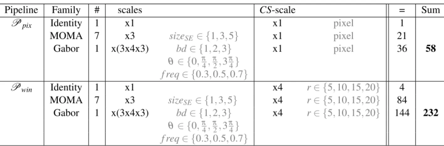
There is no parameter to be tuned for the CS when it is the pixel. For CS = sliding window however, we must set its shape and size. We will use four different sizes of square windows to

inte-Pipeline Family # scales a CS-scale = Sum

Ppix Identity 1 x1 x1 pixel 1

MOMA 7 x3 sizeSE∈ {1, 3, 5} x1 pixel 21

Gabor 1 x(3x4x3) bd∈ {1, 2, 3} x1 pixel 36 58 θ ∈ {0,π₄,π₂, 3π₄} f req∈ {0.3, 0.5, 0.7} Pwin Identity 1 x1 x4 r∈ {5, 10, 15, 20} 4 MOMA 7 x3 sizeSE ∈ {1, 3, 5} x4 r∈ {5, 10, 15, 20} 84 Gabor 1 x(3x4x3) bd∈ {1, 2, 3} x4 r∈ {5, 10, 15, 20} 144 232 θ ∈ {0,π₄,π₂, 3π₄} f req∈ {0.3, 0.5, 0.7}

Table 3.1: Recap of the features used for pipelinesPpix and Pwin. Note: MOMA stands for

“mathematical morphology operators”, Gabor for “Gabor filters”.

grate multi-scale information (radius r ∈ {5, 10, 15, 20} corresponding to squares of sizes 11×11, 21×21, 31×31 and 41×41 respectively). For operators, we take identity, the seven operators from Mathematical Morphology presented in Chapt. 2, with three scales of structuring element (V6 neighborhood), as well as Gabor filters with different bandwidths bd, directions θ and frequencies f req. This leads us to a set of 58 features forPpixand a set 232 features forPwin(see a recap in

Tab.3.1).

Remark:The lowest scale (11×11) is intended to define a support smaller than the smallest object in the image. If it is not the case, i.e. if the window is wider than the objects of interest, we advise the user to adapt the image resolution for objects to span more pixels and be more easily detected. To understand better the behavior of both pipelines, we first conduct a preliminary study on databaseD1with different families of operators.

3.2.2 Preliminary study onD1

In this subsection, we focus on the L’Oréal database. Random forest parameters are not yet opti-mized but are set to consistent values to perform the comparison (100 trees, 100 data samples at least in each leaf at the end of training). Since this database contains few images, a leave-one-out procedure is applied to evaluate the segmentation performance.

Quantitative results for both pipelines and for different families of features are presented in Tab. 3.2.

Let us start by the analysis of pipelinePpix’s performance (CS = pixel). We can see that using

only the identity is not enough to capture the main information, as classification performance is poor: F = 63%, J = 46% and Acc = 86%. This is not surprising due to the high amount of noise in these images. Moreover, the number of connected components is very high (Nb_cc = 8153 ± 147), which traduces a poor spatial coherence of detected objects. Indeed, there are, in average, five melanocytes to detect per image. The higher Nb_cc is compared to five, the more detected objects are parceled out, which is not desirable. Using families of features with richer operators, such as MOMA, enables to improve these classification performance, leading to an increase by 14% of the F-score (F = 72%) and 22% of the Jaccard index (J = 56%). The accuracy Acc only increases of 5%, but this measure should be analyzed with caution as we are dealing with a database with unbalanced classes: in the ground truth, 15% of the pixels have been assigned the label 1 and

Both offer similar classification performance. We can also notice that they notably decrease the number of connected components, even if the latter is still too high to guarantee spatial coherence of detected objects.

For the second pipelinePwin, corresponding to CS = window (4 scales), morphological

op-erators seem to be more discriminant than standard ones (F = 75% instead of F = 72%). More importantly, the comparison between both pipelines tells us that using sliding windows system-atically maintains or improves the classification performance compared to using the pixel alone. For example, the F-score obtained with the identity operator increases by 13% fromPpix

toPwin. It is also important to note that sliding windows impact more positively the spatial

co-herence of detected objects compared to pixels: for the three families, Nb_cc decreases by 95%, 28% and 50% respectively. Therefore, we can conclude, as expected, that sliding windows outper-forms the pixels taken alone because these wider supports enable to capture richer and multi-scale information in the neighborhood of the pixel to be classified.

Ω CS P R F J Acc Nb_cc Identity pixel 54 75 63 46 86 8153 ± 147 windows (4) 60 87 71 55 89 380 ± 160 Standard pixel 60 87 71 55 89 179 ± 68 windows (4) 61 87 72 56 89 129 ± 32 MOMA pixel 61 87 72 56 90 203 ± 71 windows (4) 64 89 75 59 91 101 ± 33

Table 3.2: Pixel classification: comparison between CS = pixel and CS = windows for database D1. Results are given on the test subset. Note: standard and MOMA denote usual operators used

bySommer et al.[2011] and operators from mathematical morphology respectively, all introduced in Chapt. 2.

Figure 3.6 illustrates on an image ofD1the effect of both pipelines with the three families of

features.

3.2.3 Final results on the three databases

We now evaluate the performance of the two pipelinesPpixandPwinon the three databasesD1,

D2andD3. This time, RF parameters are optimized by cross-validation (see resulting values in

Tab. A.1 of appendix A.1). The features used are those presented in Tab. 3.1.

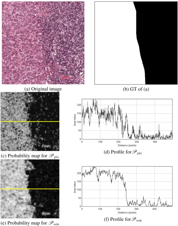
Qualitative analysis: Figures 3.7, 3.8 and 3.9 show some examples of classification results for the three databases. In Fig. 3.7, the task is to segment the tumoral region which is in the left part of the image. Corresponding probability maps are presented forPpixandPwin, along with a grey

level profile taken along the yellow line. These profiles reveal that it is easier to discriminate the two regions when using the window as CS rather than the pixel. Indeed, a wider support captures more information on the texture, a discriminant characteristic in this case. Figure 3.8 presents the probability maps for both pipelines for im1 ofD1and binary results associated to three thresholds:

0.2, 0.5 and 0.8. The higher the threshold is, the higher the confidence is to be an object pixel. Therefore, increasing the threshold value tends to decrease the number of detected pixels. We can observe that using the window as CS decreases the number of detected connected components, which traduces a better spatial coherence than for the pixel-CS. Finally, results seem to be rather

(a) Ω = Identity, CS = pixel (b) Ω = Identity, CS = windows (4)

(c) Ω = Standard, CS = pixel (d) Ω = Standard, CS = windows (4)

(e) Ω = MOMA, CS = pixel (f) Ω = MOMA, CS = windows (4)

Figure 3.6: Classification results for im1 ofD1. Legend: TP, TN, FP and FN are shown in green,

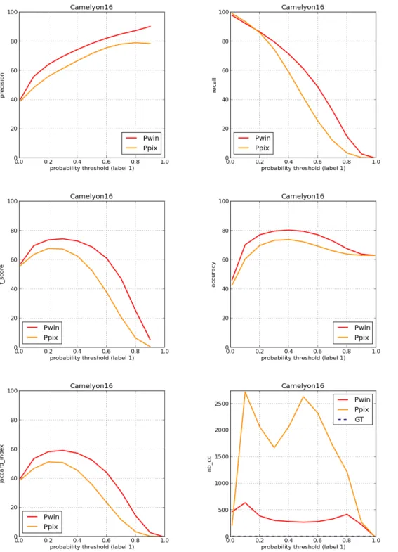
Quantitative analysis: Figures 3.10, 3.11 and 3.12 are dedicated to the quantitative evaluation of the pipelines on the three databases.D3shows the best performance andD2is more challenging,

but overall performance is already satisfactory for these two general methods. Comparing the com-putational supports, classification results are better for the window approach, except forD3where

they are equivalent. This last observation may be explained by the fact that theD3database can be

easily segmented with reasonable performance at the pixel level (a simple thresholding of pixels with positive values would even be enough, even if not perfect). The window approach is advan-tageous when contextual information around the pixel, such as texture, is needed to discriminate classes. This is also confirmed by the ROC curves presented in Fig. 3.13. Besides, for databases D1andD2,Pwinoffers a better spatial coherence, with a smaller number of detected connected

components compared toPpix. As far as specific segmentation methods are concerned, they are

equivalent (D1) or outperformed (D3) by the general approaches embodied by both pipelines.

3.3 Conclusion

To sum up, we have seen that, when performing pixel classification, using a window instead of the pixel itself as CS achieves better performance for several reasons:

• Using a wider support enables to capture richer information on the pixel to be classified. a

• Using several sizes of windows enables to capture multi-scale information, which is all the more valuable in our case as databases can present objects of different sizes and shapes. a

Yet, even the results obtained by calculating features in a sliding window could be further im-proved, regarding classification as well as spatial coherence of detected objects. In particular, this second approach mainly suffers from misclassifications on contours, as illustrated in Fig. 3.14. Figure 3.14.b is a crop on a contour of the simplified (filtered) image 3.14.a. Let us suppose that we would like to classify a pixel (shown in black in Fig. 3.14.c) with a feature consisting in taking the mean intensity value over the sliding window drawn in yellow. We can see that if the win-dow had been entirely included in the white object or in the black background, the mean intensity would have been really close to the white or to the black respectively; thus the pixel would have been easily classified as belonging to one or the other. However, for pixels lying close to a contour as in this case, the feature’s value is not representative of either class (see Fig. 3.14.d), which leads to a higher misclassification rate in this area. This contour issue is due to the fact that the computational support does not adapt to the image content.

In the following, we decide to focus on another computational support which is wider than the pixel and which adapts to the image content: the superpixel. In the next part, we will expound how to generate such a support. Eventually, we will study, in Part 3, the pertinence of its insertion in our general classification pipeline.

(a) Original image (b) GT of (a)

(c) Probability map forPpix

(d) Profile forPpix

(e) Probability map forPwin

(f) Profile forPwin

Figure 3.7: Classification results for an image ofD2. Grey level profiles are evaluated along the

(a) Probability map Ppix (b) Probability map Pwin (c) threshold = 0.2 Ppix (d) threshold = 0.2 Pwin (e) threshold = 0.5 Ppix (f) threshold = 0.5 Pwin (g) threshold = 0.8 Ppix (h) threshold = 0.8 Pwin