Kernel Based Nonlinear Canonical Analysis and
Time Reversibility
Serge Darolles
∗Jean-Pierre Florens
†Christian Gouriéroux
‡Abstract
We consider a kernel based approach to nonlinear canonical correla-tion analysis and its implementacorrela-tion for time series. We deduce a test procedure of the reversibility hypothesis. The method is applied to the analysis of stochastic differential equation from high frequency data on stock returns.
Keywords: Nonlinear Canonical Analysis, Kernel Estimators, Reversibil-ity Hypothesis, Diffusion Equations, High Frequency Data.
JEL Classification: C14, C22, C40.
∗CREST and Société Générale Asset Management. †GREMAQ and IDEI, Toulouse.
‡Corresponding Author, CEPREMAP and CREST, 15 Boulevard Gabriel Péri, 92245
Malakoff Cedex, France, tel: (33) 1 41 17 35 93, fax: (33) 1 41 17 76 66, e-mail: [email protected]
1
Introduction
Let us consider a multivariate stationary process (Xt) with a continuous
distrib-ution, denote by fhthe joint density of (Xt, Xt−h) and by f the marginal density
of Xt. Under weak conditions, the joint density can be decomposed as (see e.g.
Barrett, Lampard (1955), Dunford, Schwartz (1963), Lancaster (1968)):
fh(xt, xt−h) = f (xt)f (xt−h)[1 + ∞ i=1
λi,hϕi,h(xt) ψi,h(xt−h)], (1)
where the canonical correlations λi,h, i varying, are decreasing: λ1,h≥ λ2,h ≥
... ≥ 0, ∀h, and the canonical directions satisfy the orthogonality conditions: E[ϕi,h(Xt) ϕk,h(Xt)] = 0, ∀k = i, ∀h,
E[ψi,h(Xt)ψk,h(Xt)] = 0, ∀k = i, ∀h, (2)
E[ϕi,h(Xt)] = E[ψi,h(Xt)] = 0, ∀i,h,
and the normalization conditions:
V [ϕi,h(Xt)] = V [ψi,h(Xt)] = 1, ∀i,h.
In this note we introduce kernel based nonparametric estimators of the canonical correlations and canonical directions.
The nonlinear canonical decompositions (1) are the basis for analyzing non-linear dynamics. For instance they are used to estimate indirectly the drift and the volatility functions of an univariate stochastic differential equation from discrete time data (see Hansen, Scheinkman (1995), Kessler, Sorensen (1996), Darolles, Gourieroux (2001), Hansen, Scheinkman, Touzi (1998), Chen, Hansen, Scheinkman (1998)). They are also used to define the nonlinear autocorrelo-grams, i.e. the sequence (λi,h, h varying) (see Ding, Granger (1996),
predictor space (see Gouriéroux, Jasiak (2000)), to exhibit the dynamics of ex-treme risks in finance, and to analyze the nonlinear comovements between series, i.e. the nonlinear copersistence (see e.g. Gouriéroux, Jasiak (1999)).
In section 2 we introduce the unconstrained estimator of the canonical de-composition and describe its asymptotic properties. In section 3 we consider the corresponding estimation constrained by the reversibility property and discuss the test of the reversibility hypothesis. The method is applied in Section 4 to high frequency data on stock returns to illustrate the practical usefulness of the method. Section 5 concludes. The proofs are gathered in appendices.
2
Unconstrained estimator
We consider a pair of continuous random vectors (X, Y ), whose joint p.d.f. admits a nonlinear canonical decomposition:
f (x, y) = f (x, .)f (., y)[1 +
∞ i=1
λiϕi(x) ψi(y)], (1)
where the canonical correlations and canonical directions satisfy the standard orthogonality and normalization conditions. This decomposition exists when-ever:
Assumption A.1: f(x,.)f (.,y)f2(x,y) dxdy < +∞.
The elements of the canonical decomposition have important interpretations (see e.g. Hotelling (1936), Hannan (1961), Anderson (1963), Dauxois, Pousse (1975), Darolles, Florens, Renault (1998)). Indeed the first pair (ϕ1,ψ1) is a
so-lution of the optimization problem maxϕ,ψCorr[ϕ(X), ψ(Y )], whereas λ1is the
and λ2 the correlation between ϕ2 and ψ2, and so on. These successive
opti-mization problems are used to derive numerically the elements of the canonical decomposition.
In practice the distribution of the pair (X, Y ) is not known and the theo-retical canonical analysis cannot be performed. However we can estimate this canonical decomposition if some observations (Xn, Yn), n = 1, ..., N, of (X, Y )
are available. We assume:
Assumption A.2: The sequence (Xn, Yn), n ≥ 1, is a stationary process,
whose marginal distribution coincides with the distribution of (X, Y ).
The results will especially be applied to a stationary time series (Xt, t =
0, 1, ...) observed until date T , with Xn= Xt, Yn = Xt−h. For this reason and
without loss of generality we consider vectors X and Y with a same dimension: Assumption A.3: X and Y are d-dimensional .
2.1
Definition of the estimator
When the joint p.d.f. is unknown, we perform the nonlinear canonical analysis on a nonparametric estimator of f . We consider a kernel estimator1of this joint p.d.f. (see Rosenblatt (1956), Silverman (1986)). Let us introduce two kernels K1, K2 defined on Rd. The unknown density function is estimated by:
ˆ fN(x, y) = 1 N N n=1 1 hd 1Nhd2N K1 Xn− x h1N K2 Yn− y h2N , (2)
where h1N, h2N are the bandwidths associated with the two components. Then
we consider the associated canonical decomposition ˆλi,N, ˆϕi,N, ˆψi,N, i ≥ 1. It
1Other nonparametric estimators can be considered as sieve estimators (see
will be computed by solving the sequence of optimization problems correspond-ing to ˆfN.
In this approach ˆfN has to satisfy the properties of a density function, for
any N , to ensure the validity of the empirical canonical analysis. This justifies the next assumption.
Assumption A.4: The kernels K1, K2 are non negative, with unit mass.
2.2
Assumptions for consistency and normality of ˆ
f
NThe asymptotic properties of the estimated canonical decomposition have to be deduced from the asymptotic properties of the kernel density estimator. We consider the following assumptions to get the uniform consistency of the density kernel estimator and a central limit theorem.
Assumption A.52: The variables X and Y take values in the same compact
set X ⊂Rd, X = [0, 1]d
.
Assumption A.6: The probability density function f is continuous on X2.
Assumption A.7: The strictly stationary sequence (Xn, Yn) is geometrically
strong mixing, i.e. with α-mixing3 coefficients such that α
k ≤ c0ρk, for some
fixed c0> 0 and 0 ≤ ρ < 1.
2The compactness assumption is not restrictive. Indeed, it is always possible to transform
the initial data by a one to one transform onto a compact set, since the canonical analysis prior to transformation is easily deduced from the canonical analysis of the transformed data.
3The α-mixing coefficients α
kare defined as:
αk= sup B∈σ(Xs,s≤t) C∈σ(Xs,s≥t+k)
Assumption A.8: The kernels Ki ,i = 1, 2, are bounded, symmetric, of order
2, Lipschitzian, and satisfy lim u →∞ u dKi(u) = 0, i = 1, 2.
Assumption A.9: As N → ∞, hiN → 0, N h
d iN
(log N )2 → +∞, i = 1, 2.
Assumptions A.2-A.9 give the uniform consistency of the density kernel es-timator (see Appendix A Lemma A.1). We introduce an additional assumption to obtain the uniform consistency of the associated inner product estimator (see Appendix A Lemma A.2):
ϕ(X), ψ(Y )N = ϕ (x) ψ(y) ˆfN(x, y)dxdy.
Assumption A.10: The probability density function f is bounded from below by ε > 0.
Such assumption is now standard in the nonparametric literature (see e.g. Bosq (1998) and the references therein). If the density function were known, it would be possible to transform the data to get a uniform distribution on the compact set X = [0, 1]d. When the probability density function is unknown, a preliminary transformation can still be applied to satisfy assumption A.10, if we have a priori information on the tail behavior of the joint distribution. Without this a priori information and without assumption A.10, the results below can be strongly modified since they implicitly include a tail analysis which is out of the scope of this paper. In the special case of a Markov process (Xt), and the
choice X = Xtand Y = Xt−1, there exists another approach to circumvent the
tail problem. It consists in censoring the time series from its extreme values while performing an appropriate change of time (Darolles, Gourieroux (2001)). Indeed there is a simple relation between the canonical decompositions of the initial and transformed processes which can be exploited.
We now introduce the assumptions needed to derive a central limit theorem for the kernel density estimator.
Assumption A.11: The p.d.f. ft1,t2,t3,t4 of {(Xt1, Yt1), (Xt2, Yt2), (Xt3, Yt3),
(Xt4, Yt4)} exists for any t1< t2< t3< t4, and supt1<t2<t3<t4 ft1,t2,t3,t4 ∞<
∞.
Assumption A.12: The p.d.f. ft1,t2 of {(Xt1, Yt1), (Xt2, Yt2)} satisfies the
condition supt1<t2 ft1,t2− f ⊗ f ∞< ∞, where f ⊗ f denotes the product of
marginal p.d.f. of (Xti, Yti), i = 1, 2.
Assumption A.13: The p.d.f. f is twice continuously differentiable on ]0, 1[2d, and there exists b such that f ∞< b and f(2)
∞< b.
Assumption A.14: As N → ∞, hiN → 0, NhdiN → ∞, Nh d+4
iN → 0, i = 1, 2.
Assumptions A.2-A.8 and A.11-A.14 allow to derive a central limit theorem and then obtain the asymptotic distribution of the kernel density estimator (see Appendix B Lemma B.1).
2.3
Consistency of the estimated canonical analysis
We are concerned by the consistency of the p first estimated canonical cor-relations and canonical directions, i.e. their convergence to their theoretical counterparts. We first need to introduce some identifiability conditions. Assumption A.15: The p first canonical correlations are distinct.
Assumption A.15 is an identifiability condition for the canonical correla-tions. Since ∞i=1λ2i = f (x,.)f (.,y)f2(x,y) dxdy < +∞, distinct nonzero canonical correlations are necessarily isolated. Another identifiability assumption has to
be introduced for the canonical directions, which are defined up to a change of sign.
Assumption A.16: There exists a value x0such that ϕj(x0) = 0, j = 1, ..., p.
Hence we select the pair of canonical directions with ˆϕjN(x0) > 0 and
ϕj(x0) > 0, j = 1, ..., p.
Moreover the functional parameters of interest have to belong to the admis-sible values of the associated estimators. Note that the initial and approximated optimization problems associated with the nonlinear canonical analysis are not defined on the same spaces of functions. Indeed the approximated optimizations involve the spaces L2N(X), L2N(Y ) of square integrable functions with respect to
ˆ
fN. A function ϕ is square integrable in the approximated optimization problem
of order N if and only if: ϕ2(x) 1 hd 1N
K1 Xn− x
h1N dx < +∞, n = 1, ..., N.
Since the observations can take any value from the support of the marginal distribution of f and the bandwidth may vary, it is useful to introduce the following space: L2K1(X) = {ϕ : ϕ 2(x) 1 hd 1 K1 ˜ x − x h1 dx < +∞, ∀h1> 0, ∀˜x ∈ supp f}, the space L2
K2(Y ) being defined accordingly. The links between the spaces
L2
K1(X) and L
2(X) (L2
K2(Y ) and L
2(Y ) respectively) involve the respective
tails of the kernels K1, K2 and the p.d.f. f . We intuitively have to select
kernels with rather thin tails to be sure that L2K1(X) includes the theoretical canonical directions of interest. It explains the assumption below.
Assumption A.17: The canonical directions ϕi and ψj are such that ϕi∈ L2
K1(X) , i = 1, ..., p, and ψj∈ L
2
Finally the assumption below is useful to study the estimators in appropriate topological space.
Assumption A.18: i) The canonical variates ϕi, ψi, i = 1, ..., p, are continu-ouly differentiable.
ii) The kernels K1, K2 are continuously differentiable.
Theorem 2.1 : Under the identification conditions A.15 and A.16, the estima-bility conditions A.17-A.18 and the technical assumptions A.1-A.10, ˆλi,N, ˆϕi,N,
ˆ
ψi,N, i = 1, ..., p converge to their theoretical counterparts in the sense:
ˆ λi,N →
N→∞λi a.s.
| ˆϕi,N(x) − ϕi(x) |2f (x, .)dx →
N→∞0 a.s.,
| ˆψi,N(y) − ψi(y) |2f (., y)dy →
N→∞0 a.s..
Proof. See Appendix A.
The a.s. convergence of the integrated mean square error does not imply in general the a.s. pointwise convergence of the estimated canonical variates. It implies (under some additional assumptions) the convergence of inner products < ˆϕi,N, g >, for any test function g ∈ L2(X) (see Darolles, Florens, Renault
(2001)). However, to obtain simple pointwise asymptotic distributions, we only consider x for which the pointwise convergence is achieved.
2.4
Asymptotic distributions
The convergence properties of the estimated canonical correlations and canon-ical directions allow us to expand the first order conditions and to derive the asymptotic distributions.
Theorem 2.2 : Under assumptions A.1-A.18,
i) the asymptotic distribution of ˆλN = (ˆλ1,N, ..., ˆλp,N) is a gaussian
distri-bution:
√
N (ˆλN− λ) d
→ N (0, V ),
where the elements of the matrix V are: Vi,j = 14 ∞k=−∞Cov[2ϕi(Xn)
ψi(Yn) − λiϕi2(Xn) − λiψ2i(Yn) , 2ϕj(Xn+k) ψj(Yn+k) − λjϕ2j(Xn+k) −
λjψ2j(Yn+k)].
ii) The asymptotic distribution of ˆϕN(x) = (ˆϕ1,N(x), ..., ˆϕp,N(x)) is a gaussian distribution:
N hd
1N(ˆϕN(x) − ϕ (x)) d
→ N (0, W (x)),
where Wi,j(x) = λi1λjf (x,.)1 K12(u) du Cov[ψi(Y ) , ψj(Y ) | X = x].
iii) The asymptotic distribution of ˆψN(y) = (ˆψ1,N(y), ..., ˆψp,N(y)) is a gaussian distribution:
N hd
2N( ˆψN(y) − ψ(y)) d
→ N (0, U(y)),
where Ui,j(y) = λi1λjf (.,y)1 K22(u) du Cov[ϕi(X) , ϕj(X) | Y = y].
Proof. See Appendix B
The rate of convergence is a parametric rate for the canonical correlations, whereas it is nonparametric for the canonical directions. The asymptotic vari-ance Wi,i(x) of ˆϕi,N coincides with the asymptotic variance of the
Nadarahya-Watson estimator of λ1
iE[ψi(Y ) | X]. This corresponds to the interpretation
of the canonical direction ϕi as the conditional expectation of the canonical direction ψi, up to a scale factor.
3
The reversibility hypothesis
In this section we are interested in reversible processes, i.e. processes with identical distributional properties in initial and reversed times. Discretized uni-dimensional diffusion processes are examples of reversible processes. Therefore, when rejecting the reversibility hypothesis, we also reject the existence of an underlying unidimensional diffusion process (see section 4). Some other pro-cedures to test for unidimensional diffusion processes have been based on the embeddability hypothesis (see Florens, Renault, Touzi (1998)).
The reversibility condition implies that, ∀h, fh(xt, xt−h) = fh(xt−h, xt),
i.e. the symmetry of the bivariate distribution fh at any lag. We explain in
the subsection below how to estimate the canonical decomposition of f (x, y) under these reversibility (i.e. symmetry) conditions. Then, by comparing the unconstrained and constrained estimators, we derive a test of the symmetry hypothesis.
3.1
Constrained estimators
There exists different kernel estimators of the canonical decomposition taking into account the symmetry constraint.
i) We select identical kernels K1= K2= K and bandwidths h1N= h2N = hN,
whereas we artificially double the size of the sample by considering (Xi, Yi),
(Yi, Xi), i = 1, ..., N . The constrained kernel estimator of the density function
is: ˆ fNR(x, y) = 1 2N h2d N N n=1 {K Xnh− x N K Yn− y hN +K Xn− y hN K Yn− x hN }.
di-rections are deduced from the canonical decomposition of ˆfR
N and denoted by
ˆ
λRi,N and ˆϕRi,N = ˆψRi,N, i ≥ 0.
ii) We look for the solutions of the spectral problem: 1
2( ˆT
∗+ ˆT )ˆϕR i,N = ˆλ
R
i,NϕˆRi,N, ˆϕRi,N, ˆϕRi,N = 1,
where: ˆ T ϕ(y) = ϕ(x)fˆN(x, y) ˆ fN(., y) dx, ˆ T∗ϕ(x) = ϕ(y)fˆN(x, y) ˆ fN(x, .) dy. iii) We look for the solutions of the spectral problem:
1 2( ˆT
∗T + ˆˆ T ˆT∗)ˆϕR i,N = (ˆλ
R
i,N)2ϕˆRi,N, ˆϕRi,N, ˆϕRi,N = 1.
The latter approaches are based on the property of self-adjoint conditional expectation operator under the reversibility hypothesis. These three constrained estimators do not provide the same results in finite sample, but share the same asymptotic properties under the reversibility hypothesis.
Theorem 3.1 : Under the assumptions of theorem 2.2, and if the reversibility hypothesis is satisfied,
i) ˆλRi,N, ˆϕRi,N, i = 1, ..., p, converge a.s. to their theoretical counterparts.
ii) The asymptotic distribution of ˆλRN = (ˆλR1,N, ..., ˆλRp,N) is a gaussian distri-bution: √ N (ˆλRN− λ)→ N (0, Vd R), where VR i,j = 14 ∞k=−∞Cov[2ϕi(Xn) ϕi(Yn) − λiϕ2i(Xn) − λiϕ2i(Yn) , 2ϕj(Xn+k) ϕj(Yn+k) − λjϕ2j(Xn+k) − λjϕ2j(Yn+k)].
iii) The asymptotic distribution of ˆϕRN(x) = (ˆϕR1,N(x), ..., ˆϕRp,N(x)) is a gaussian distribution: N hd N(ˆϕ R N(x) − ϕ (x)) d → N (0, WR(x)), where WR i,j(x) = 12 1 λiλj 1 f (x,.) K 2 1(u) du Cov[ϕi(Y ) , ϕj(Y ) | X = x].
Proof. See Appendix C.
We obtain asymptotic results, which may be directly compared to Theorem 2.2. The constrained and unconstrained estimators of the canonical correlations have the same asymptotic distribution under the reversibility hypothesis. In contrast the asymptotic variance of the constrained estimated canonical variate is half the variance of the unconstrained one. This is a correction for the double size of the sample (see interpretation i) of the constrained estimator).
3.2
Comparison of constrained and unconstrained
estima-tors
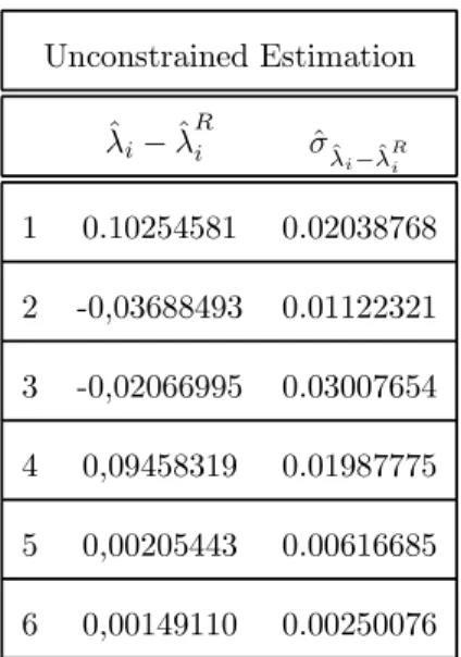
Under the null hypothesis of reversibility we can compare the asymptotic proper-ties of the constrained and unconstrained estimators of the canonical correlations and canonical directions. The difference between these two types of estimators can be used to construct testing procedures of the reversibility hypothesis.
3.2.1 Asymptotic equivalence
Under the reversibility hypothesis, ˆλ1N and ˆλ R
1N admit the same first order
expansion. Therefore we need the second order expansion of the difference ˆ
λ1N − ˆλ R
Appendix D. The notation ∼ means that the residual term can be neglected with respect to the terms of the left and right hand sides.
Theorem 3.2 : Under the reversibility hypothesis, we have the asymptotic equivalences: 2(ˆϕ1N− ˆϕR1N) ∼ ˆϕ1N− ˆψ1N, and ˆ λ1N− ˆλ R 1N ∼ 2λ1 ϕˆ1N(y) − ˆϕR1N(y) 2 f (., y)dy ∼ λ1 2 ϕˆ1N(y) − ˆψ1N(y) 2 f (., y)dy.
Proof. See Appendix D.
The first relation means that it is equivalent to construct a test procedure based on the difference between the constrained and unconstrained estimators of the canonical variates ϕ1, or the difference between the unconstrained esti-mators of the canonical variates ϕ1 and ψ1. The second equation shows that a testing procedure based on the difference between the constrained and uncon-strained canonical correlations consists in introducing an appropriate measure of discrepancy between the estimators of ϕ1.
3.2.2 Test procedure
A test procedure can be deduced from the asymptotic properties of:
IN= µ1 ϕˆ1N(y) − ˆψ1N(y)) 2
f (., y)dy. (3)
The difference between ˆϕ1N and ˆψ1N has been weighted by the marginal distribution f (., y) to keep the interpretation of Theorem 3.2. Similar results can be derived if f (., y) is replaced by another weighting function w(y) (see e.g.
Hall (1984a), Tenreiro (1997)). For instance we may use w(y) = f2(., y) (see
Pagan, Ullah (1999), p. 168).
The analysis is similar to the one usually followed for the integrated square error of nonparametric density or regression estimators (see e.g. Bickel, Rosen-blatt (1975), Nadaraya (1983), Hall (1984a), Hall (1984b)). However these results are generally derived for i.i.d. observations, and we will use an extension of limit theorems established by Tenreiro (1997) (see also Meloche (1990)).
We assume that the process Zi = (Xi, Yi) is strongly stationary and
geo-metrically absolutely regular (see Bradley (1986)). Then, under regularity con-ditions described in Appendix E, we get the theorem below:
Theorem 3.3 : Under the reversibility hypothesis,
i) the asymptotic distribution of IN− EIN is a gaussian distribution:
N hd/2N (IN− EIN) d → N (0, η2), where: η2= 2 K(u)K(u + v)du 2 dv (V ar [ϕ1(Xi+1) | Xi= xi])2dxi.
ii) The bias is: EIN = 2 Nhd N K2(u)du V ar [ϕ1(Xi+1) | Xi= xi] dxi+ o 1 N hdN−1 . After replacement of INby a consistent estimator, we deduce from Theorem
3.3 a procedure for testing the reversibility hypothesis.
The test procedures described above can be used to check if discrete time data are compatible with an underlying continuous time diffusion model. To solve the question we can proceed in two steps. First apply a test for embed-dability (see e.g. Florens, Renault, Touzi (1998)) to check if the eigenvalue are
stricly positive, that is if the data are compatible with a continuous time model (not necessarely a diffusion). If the the embeddability hypothesis is not rejected, the reversibility test can then be performed.
4
Applications
In this section we provide two illustrations of the approach. The first one is based on an artificial dataset consisting of simulated realizations of a reflected Brownian motion. This is a Markov reversible process providing a basis for a comparison of different estimation techniques. The second example involves high frequency data on returns on the Alcatel stock traded on the Paris-Bourse.
4.1
Reflected Brownian motion
In this example we consider a reflected Brownian motion, with zero drift, a variance σ2, and two reflecting barriers at 0 and l. This process is stationary,
markovian and reversible. Its infinitesimal generator:
Af (x) = lim h→0 E [f (Xt+h) | Xt= x] − f (x) h = 1 2σ 2 d2 dx2f (x), (4)
is defined for any function f belonging to D (Λ) = f ∈ L2: Af exists and
f (0) = f (l) = 0}, where L2 is the space of square integrable functions with respect to Lebesgue measure on [0, l]. The eigenelements (ρi, ei) of A are (see
Darolles, Laurent (2000) for the computation):
ρi= −1 2 iσπ l 2 , ei(x) = cos iπ l x , i varying.
Therefore, the canonical variates associated with discrete observations (Xt,
are λi = exp(ρi), i = 1 varying. Moreover the reflected Brownian motion is
reversible.
We simulate a path (Xt, t = 1, 2, ..., T ) of length T = 2500, for the volatility
σ = 1 and the barrier l = π. Next, we use these artificial observations to find the nonlinear canonical decomposition of the joint distribution of (Xt, Xt−1). Two
estimation methods are successively applied to the data (Xt, Xt−1), t = 2, ..., T :
i) an unconstrained kernel method, with gaussian kernels K1(x) = K2(x),
and bandwidths h1= h2= 0.1025;
ii) the same kernel method constrained by the reversibility hypothesis.
We provide the estimated canonical correlations in Table 4.1.
[Insert here Table 4.1: Estimated canonical correlations]
The constrained and unconstrained estimators of the canonical correlations are close to each other, and close to the true values. Similar results are obtained when comparing the estimators of the canonical variates. Hence we only consider below the constrained estimation method.
[Insert here Figure 4.1: Constrained kernel estimator of the first canonical variate]
To study the asymptotic variance of the estimators, we perform the following Monte-Carlo study. We replicate 250 simulated paths using the same parameters values and we compute at each point of the support the mean and the standard deviation of the estimator of the first canonical variate. Figures (4.1) and (4.2)
provide the averaged estimators and the pointwise confidence bands, computed for the first and the second canonical variates. The figure presents the true function (dotted line) and its estimator (continuous line).
[Insert here Figure 4.2: Constrained kernel estimator of the second canonical variate]
The kernel estimators of the canonical variates satisfy approximatively the boundary constraints ϕ1(0) = ϕ1(l) = 0 . This nice property is not satisfied in practice by the standard sieve method, which can create important finite sample bias (see Darolles, Gouriéroux (1997) for a modification of the sieve approach to integrate the boundary effects).
4.2
High Frequency Data
We consider a series of returns corresponding to the Alcatel stock traded on the Paris-Bourse. The prices are resampled every 20mn from real time records and the returns are computed by differencing the log-prices. The observation period is May 2, 1997, to August 30, 1997, and includes 1705 observations. For this application, we can assume that returns take values in a compact set. Indeed, the tradings would automatically stop if the price modification with respect to the opening price was too large.
[Insert here Table 4.2: Estimated canonical correlations]
We implement the unconstrained and constrained kernel based methods, with a gaussian kernel and bandwidths h1N = h2N = 0.062. The
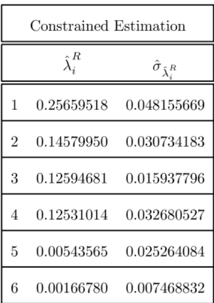
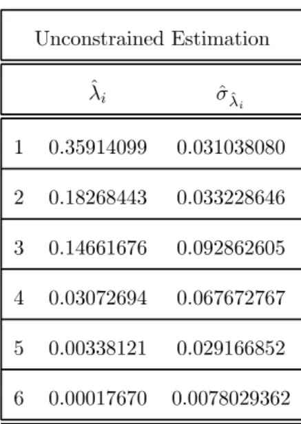
reversibil-ity hypothesis is clearly rejected when we compare the constrained and un-constrained estimated canonical correlations (see Table 4.2, their asymptotic variances are provided in Appendix F ). The introduction of the reversibil-ity constraint induces an underestimation of the first canonical correlation by about 30%.
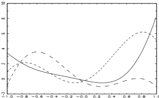
[Insert here Figure 4.3: Estimated current canonical variates]
The estimated canonical variates are provided in Figures (4.3) and (4.4) for the unconstrained case. The first variate is represented by a continuous line, the second one by a dashed line, and the third one by a dotted line.
[Insert here Figure 4.4: Estimated lagged canonical variates]
It is commonly assumed in financial theory that the stock returns (Xt, t ≥ 0)
satisfy a stochastic differential equation:
dXt= µ (Xt) dt + σ (Xt) dWt, (say).
In such a case the process is necessarily reversible and the first canonical variate corresponds to a monotonous function, the second one to a function with one breakpoint, and so on. The comparison of the three figures shows clearly that the reversibility property has to be rejected, as the expected patterns of the canonical variates are. In particular, the observed returns are not compatible with an underlying unidimensional stochastic differential equation.
How to interpret the pattern of the first canonical variate ? It is well known that the (linear) autocorrelations of stock returns are generally insignificant,
which is consistent with the theory of market efficiency. In our case the first order linear correlation is 0.065 and is not significant. Therefore the linear trans-formation will not belong to the subspaces generated by the first canonical vari-ates. Moreover the literature on ARCH models insists on the so-called volatility persistence, implying a large autocorrelation of squared returns. Therefore it is not surprising to find a first canonical variate with a parabolic form, even if the pattern also includes some leverage effect (see Black (1976)).
5
Concluding Remarks
In this paper we develop a nonlinear canonical correlation analysis based on kernel estimators of the density function. It allows to define nonparametric estimators of the canonical correlations and canonical directions either un-constrained, or constrained by the reversibility property. This nonparametric canonical analysis is especially useful for financial applications based on high frequency data and for the estimation of the drift and volatility functions of a diffusion equations. It may also be used to study the liquidity risk in an analy-sis of intertrade durations (see Gouriéroux, Jasiak (1998)), or to implement technical analysis based models for directions of price changes (see Darolles, Gourieroux, Le Fol (2000)).
A
Proof of Theorem 2.1
From Roussas (1988), theorem 3.1, Bosq (1998), theorem 2.2, we get the follow-ing lemma.
is uniformly strongly consistent.
From this result, we deduce a uniform consistency property of integrals with respect to ˆfN.
Lemma A.2 : Under assumptions A.2-A.10, g(x, y) ˆfN(x, y)dxdy converges
a.s. uniformly to g(x, y)f (x, y)dxdy, for any function g in G = {g : |g(x, y)| f (x, y)dxdy ≤ 1}.
Proof. For any function g in G = {g : |g(x, y)| f(x, y)dxdy ≤ 1}, we get: supg∈G | g(x, y)[ ˆfN(x, y) − f(x, y)]dxdy |≤ sup(x,y)∈X2 | ˆfN(x, y) − f(x, y) |
/f (x, y). Using assumption A.10, this uniform convergence is equivalent to the uniform convergence of ˆfN(x, y) to f (x, y) given by Lemma A.1.
Let us now prove the consistency for i = 1. The case i = 1 can be easily de-duced by similar arguments. Let us introduce the three following maximization problems:
Problem A.1: (ˆϕ1,N, ˆψ1,N) solution of maxϕ,ψ ϕ (x) ψ(y) ˆfN(x, y)dxdy,
sub-ject to ϕ2(x) ˆf
N(x, .)dx = ψ2(y) ˆfN(., y)dy = 1.
Problem A.2: (˜ϕ1,N, ˜ψ1,N) solution of maxϕ,ψ ϕ (x) ψ(y) ˆfN(x, y)dxdy,
sub-ject to ϕ2(x) f (x, .) dx = ψ2(y)f (., y)dy = 1.
Problem A.3: (ϕ1, ψ1) solution of maxϕ,ψ ϕ (x) ψ(y)f (x, y)dxdy, subject to
ϕ2(x) f (x, .)dx = ψ2(y)f (., y)dy = 1.
Let us denote H ={(ϕ, ψ) : ϕ2(x) f (x, .)dx = ψ2
(y) f (., y)dy = 1}. We first prove the consistency of ˜ϕ1,N and ˜ψ1,N.
Using Cauchy-Schwarz inequality, we get g(x, y) = ϕ (x) ψ(y) ∈ G, ∀(ϕ, ψ) ∈ H, and by Lemma A.2 we deduce the a.s. uniform convergence ϕ (x) ψ(y)
ˆ
fN(x, y)dxdy → ϕ (x) ψ(y)f (x, y)dxdy as N → ∞. Moreover the application
(ϕ, ψ) → ϕ (x) ψ(y)f (x, y)dxdy, is continuous from L2(X) ×L2(Y ) to R. We use a Jennrich’s lemma valid for any metric space (see Jennrich (1969), proof of Theorem 6) to deduce the a.s. convergence of the solutions of the finite sample problem to the solution of the limit problem A.3. This implies:
˜
ϕ1,N−ϕ1 2→ 0 a.s. and ˜ψ1,N−ψ1 2→ 0 a.s., where . 2is the L2distance.
ii ) Consistency of ˆϕ1,N and ˆψ1,N
Since g(x, y) = ϕ2(x) ∈ G and g(x, y) = ψ2
(y) ∈ G, when (ϕ, ψ) ∈ H, we deduce from Lemma A.2 the equicontinuity property, which implies the a.s. convergences: αN = ϕ˜21,N(x) ˆfN(x, .)dx → ϕ21(x) f (x, .) dx = 1, a.s., and
βN = ψ˜21,N(y) ˆfN(., y)dy → ψ21(y)f (., y)dy = 1, a.s.. The solutions (˜ϕ1,N,
˜
ψ1,N) and (ˆϕ1,N, ˆψ1,N) of problems A.1 and A.2 are proportional up to the terms (α1/2N , β1/2N ). Therefore we have ϕˆ1,N − ϕ1 2 ≤ ˜ϕ1,N− ϕ1 2+ (1 − α−12
N )˜ϕ1,N 2 = ϕ˜1,N − ϕ1 2+ | 1 − α −1
2
N |, and we deduce ˆϕ1,N− ϕ1 2 → 0
a.s. A similar computation gives the consistency of ˆψ1,N. iii ) Consistency of ˆλ1,N
It is a consequence of the equicontinuity property.
B
Proof of Theorem 2.2
From Bosq (1998), theorem 2.3, we get the following central limit theorem for the kernel density estimator.
N hd
2Nhd1N[ ˆfN(x, y) − f(x, y)] d
→ N (0, W (x, y)), where W (x, y) = f(x, y) K12(u) du K22(u) du.
To derive the asymptotic distributions, we need central limit theorems for specific transformations of the kernel density estimator.
Lemma B.2 : Under assumptions A.2-A.8, A.11-A.14, we get for a given function g(x, y):
i) √N g(x, y)[ ˆfN(x, y) − f(x, y)]dxdy → N (0, V ), with asymptotic varianced
V = ∞
k=−∞Cov[g (Xn, Yn) , g (Xn+k, Yn+k)].
ii) N hd
1N g(x, y)[ ˆfN(x, y)−f(x, y)]dy d
→ N (0, W (x)), with asymptotic vari-ance W (x) = K12(u) du g2(x, y)f (x, y)dy.
iii) If the reversibility hypothesis is satisfied, Nhd
N g(x, y)[ ˆfNR(x, y) − f(x, y)]dy d
→ N (0, W (x)), with asymptotic vari-ance W (x) = 12 K2(u) du g2(x, y)f (x, y)dy.
We can now begin the proof of theorem 3.2. We derive asymptotic distrib-utions for p = 1. The case p = 1 is easily deduced by similar arguments. i) Expansion of the first order condition
Let us denote by L2(X) (resp. L2(Y )) the space of square integrable functions
of X (resp. Y ), by . 2the associated L2norm, by T the conditional expectation
operator from L2(X) to L2(Y ):
T : ϕ (X) → T ϕ (Y ) = E[ϕ (X) | Y ] = ϕ (x)f (x, y) f (., y)dx, and by T∗ the adjoint operator of T :
T∗: ψ (Y ) → T ψ (X) = E[ψ (Y ) | X] = ψ(y)f (x, y) f (x, .)dy.
The first order conditions associated with Problem A.3 are: T∗T ϕ 1= µ1ϕ1 and T T∗ψ 1= µ1ψ1, where µ1= λ 2 1. Moreover ϕ1, ϕ1 = 1, ψ1, ψ1 = 1, and: T ϕ1= µ12 1ψ1, T∗ψ1= µ 1 2 1ϕ1. T , T∗, ϕ
1, ψ1 and µ1 are function of the distribution F . We denote by
dTF(H) (resp. dTF∗(H), dϕ1F(H), dµ1F(H)) the Gâteaux derivative of T (resp.
T∗, ϕ
1, µ1) in the direction H at the point F (h(x, y) denotes the p.d.f. of H).
We will derive the explicit expressions of dµ1F(H) and dϕ1F(H). The Gâteaux derivative of the first order condition corresponding to µ1 and ϕ1is:
dµ1F(H)ϕ1= dTF∗(H)T ϕ1+ T∗dTF(H)ϕ1+ (T∗T − µ1I)dϕ1F(H), (5)
where I is the identity operator. i.a) Expression of dµ1F(H)
Let us focus on dµ1F(H). To eliminate the term dϕ1F(H) in the expression above, we compute the inner product of this equation with ϕ1. We find: dµ1F(H) ϕ1, ϕ1 = ϕ1, (dTF∗(H)T +T∗dTF(H))ϕ1 + ϕ1, (T∗T −µ1I)dϕ1F(H) .
By the normalization condition ϕ1, ϕ1 = 1, its derivative satisfies: ϕ1, dϕ1F(H) = 0.
Moreover by using the definitions of the adjoint operator and of ψ1, we get:
dµ1F(H) = µ
1 2
1[ ϕ1, dTF∗(H)ψ1 + ψ1, dTF(H)ϕ1 ]. (6)
Let us now compute the quantities dTF(H)ϕ1(y) and dTF∗(H)ψ1(x). We get:
dTF(H)ϕ1(y) = ϕ1(x) h(x, y) f (., y) − f (x, y) f (., y)2h(., y) dx = 1 f (., y) ϕ1(x)h(x, y)dx − T ϕ1(y)h(., y) = 1 f (., y) (ϕ1(x) − µ 1 2 1ψ1(y))h(x, y)dx,
and dTF∗(H)ψ1(x) = 1 f (x, .) (ψ1(y) − µ 1 2 1ϕ1(x))h(x, y)dy. (7)
By introducing this expression in condition (6), we get the expression of dµ1F(H) as an integral with respect to h:
dµ1F(H) = µ12 1 [2ϕ1(x)ψ1(y) − µ 1 2 1ϕ21(x) − µ 1 2 1ψ21(y)]h(x, y)dxdy. (8) i.b) Expression of dϕ1F(H) From (5), we get: (µ1I − T∗T )dϕ1F(H) = dTF∗(H)T ϕ1+ T∗dTF(H)ϕ1− dµ1F(H)ϕ1 = dTF∗(H)T ϕ1+ T∗dTF(H)ϕ1− ϕ1, dTF∗(H)T ϕ1+ T∗dTF(H)ϕ1 ϕ1.
The r.h.s. belongs to the null space of the operator µ1I −T∗T , which implies
the existence of a solution dϕ1F(H). Moreover the solution is unique due to the constraint ϕ1, dϕ1F(H) = 0. It satisfies the Fredholm equation:
(µ1I − T∗T )dϕ1F(H) = dvF(H),
where dvF(H) denotes the r.h.s.. It can be written as:
dϕ1F(H)(x) = 1
µ1dvF(H) − b(x, s)dvF(H)ds, where: b(x, s) = µ1
1 j=1
µ1
µ1−µkϕj(x) ϕj(x). Assumption A.15 ensures the
convergence of the series defining b. i.c) Frechet differentiability
The directional Gâteaux derivatives can be used to derive the first order ex-pansions of µ1(F + H) − µ1(F ), ϕ1(F + H) − ϕ1(F ) and ψ1(F + H) − ψ1(F ), whenever these functions are Frechet differentiable.
Let us consider the canonical variate ϕ1(F ) which is solution of the implicit equation:
TF∗TFϕ1− TFϕ1, TFϕ1 Fϕ1= 0.
It is easily checked that the application:
g : (F, ϕ) → TF∗TFϕ − TFϕ, TFϕFϕ
is Frechet differentiable for the L2(X) norm for ϕ and g, and the norm:
F (∞,1)= sup
x,y |F (x, y)| + supx,y d i=1 ∂F ∂xi (x, y) + sup x,y d i=1 ∂F ∂yi (x, y) ,
for F . We deduce the differentiability of ϕ1 with respect to F by the implicit function theorem. Indeed we have:
∂g
∂ϕ(F, ϕ1)dϕ1F = (T
∗T − µ
1I)dϕ1F = 0.
Similarly we can check that:
µ1(F ) = max
ϕ,ψ TFϕ, ψ F,
where the maximum is computed on the pair (ϕ, ψ) of continuously differentiable functions, is Frechet differentiable for the norm:
F (∞,0)= sup
x,y|F (x, y)| ,
for F and the standard norm of R for µ. ii) Asymptotic distribution of ˆλ1,N
By the Frechet differentiability of µ1(F ) and the assumption A.18, we deduce the first order expansion of ˆµ1,N. We have:
ˆ
and: √
N (ˆµ1,N− µ1) =√N dµ1F( ˆFN− F ) + o
√
N ˆFN− F (∞,0) .
Since √N ˆFN − F (∞,0) = Op(1) (see Aït-Sahalia (1992), proof of
theo-rem 2), the two terms √N(ˆµ1,N − µ1) and √N dµ1F( ˆFN− F ) have the same
asymptotic distribution. We get: √ N dµ1F( ˆFN− F ) = √ N µ 1 2 1[2ϕ1(x)ψ1(y) − µ 1 2 1ϕ21(x) − µ 1 2 1ψ 2 1(y)] ×[ ˆfN(x, y) − f(x, y)]dxdy,
and the asymptotic distribution of ˆµ1,Nfollows from Lemma B.2 i) with g(x, y) = µ 1 2 1[2ϕ1(x)ψ1(y) − µ 1 2 1ϕ21(x) − µ 1 2 1ψ 2
1(y)]. We immediately deduce the asymptotic
distribution of ˆλ1,N= (ˆµ1,N)
1 2.
iii) Asymptotic distribution of ˆϕ1,N
By the Frechet differentiability of ϕ1(F ) and the assumption A.18, we deduce the first order expansion of ˆϕ1,N.We get:
ˆ ϕ1,N− ϕ1= ϕ1( ˆFN) − ϕ1(F ) = dϕ1F( ˆFN− F ) + o FˆN− F (∞,1) , and Nhd 1N(ˆϕ1,N− ϕ1) = Nhd1Ndϕ1F( ˆFN− F ) + o N hd1N FˆN− F (∞,1) . Since N hd
1N FˆN− F (∞,1)= Op(1) (see Aït-Sahalia (1992), proof of
the-orem 3), N hd
1N(ˆϕ1,N− ϕ1) and N hd1Ndϕ1F( ˆFN− F ) have the same
asymp-totic distribution (see Serfling (1980), Lemma B p. 218). Moreover by using the expression of dϕ1F(H) and comparing the rates of convergence, we get:
N hd 1Ndϕ1F( ˆFN− F )(x) = 1 µ1 Nh d 1NdTF∗(H)T ϕ1(x) + op(1) = 1 λ1 1 f (x, .) N h d 1N [ψ1(y) − λ1ϕ1(x)] ×[ ˆfN(x, y) − f(x, y)]dy + op(1). (9)
We apply Lemma B.2 ii) with g(x, y) =λ1
1
1
f (x,.)[ψ1(y) − λ1ϕ1(x)] to get the
asymptotic distribution of ˆϕ1,N(x): N hd 1N(ˆϕ1,N(x) − ϕ1(x)) d → N (0, W1,1(x)), where W1,1(x) = K12(u) du 1 λ21 1 f2(x, .) [ψ1(y) − λ1ϕ1(x)]2f (x, y)dy = 1 λ21 1 f (x, .) K 2 1(u) du V [ψ1(Y ) | X = x].
The proof is similar for deriving the asymptotic distributions of (ˆϕ1,N(x) , ... , ˆϕp,N(x)) and of (ˆψ1,N(x) , ..., ˆψp,N(x)).
C
Proof of Theorem 3.1
The proof of consistency is similar to the proof given for theorem 2.1 in Appen-dix A. We derive asymptotic distributions of the estimators under the reversibil-ity hypothesis. We only present the expansions for the constrained estimators of type iii) defined by:
1 2( ˆT
∗T + ˆˆ T ˆT∗)ˆϕR
i,N = ˆµRi,NϕˆRi,N, ˆϕRi,N, ˆϕRi,N = 1,
where ˆµRi,N = (ˆλRi,N)2. For expository purpose, we consider the case p = 1. The
Gâteaux derivative of the first order condition is:
dµR1F(H)ϕ1= 1 2d(T ∗ FTF + TFTF∗)(H)ϕ1+ ( 1 2(T ∗T + T T∗) − µ 1I)dϕR1F(H).
re-versibility hypothesis and is such that T∗= T , ϕ 1= ψ1. We get: dµR1F(H)ϕ1 = 1 2[dT ∗ F(H)T + T dTF(H) + dTF(H)T + T dTF∗(H)] ϕ1 +(T2− µ1I)dϕR1F(H), (10) where I is the identity operator.
i) Expression of dµR 1F(H)
To eliminate the terms dϕ1F(H) in the previous expression, we compute the inner product of this equation with ϕ1. We find:
dµR1F(H) = µ
1 2
1[ ϕ1, dTF∗(H)ϕ1 + ϕ1, dTF(H)ϕ1 ]. (11)
By comparing with the Gâteaux derivative of the unconstrained estimator (see appendix B), we note that:
dµR1F(H) = dµ1F(H),
under the reversibility hypothesis. In particular the constrained and uncon-strained estimated canonical correlations have the same asymptotic distribu-tions. ii) Expression of dϕR 1F(H) From (10), we get: (µ1I − T2)dϕR 1F(H) = dvFR(H), where dvRF(H) = 1 2[(dT ∗ F(H) + dTF(H))T + T (dTF∗(H) + dTF(H))] ϕ1− dµR1F(H)ϕ1.
of convergence, we get: Nhd Ndˆϕ R 1,N( ˆFN− F )(y) = Nhd N µ1 1 2 dT ∗ F( ˆFN− F ) + dTF( ˆFN− F ) T ϕ1(y) + op(1) = Nh d N λ1 1 f (., y) (ϕ1(x) − µ 1 2 1ϕ1(y)) ˆ fN(x, y) + ˆfN(y, x) 2 − f(x, y) dx + op(1) = Nh d N λ1 1 f (., y) (ϕ1(x) − µ 1 2 1ϕ1(y)) ˆfNR(x, y) − f(x, y) dx + op(1).
We apply Lemma B.2 iii) with g(x, y) =λ1
1
1
f (.,y)[ϕ1(x) − λ1ϕ1(y)] to obtain
the asymptotic distribution of ˆϕR1,N: N hd N(ˆϕ R i,N(x) − ϕi(x)) d → N (0, W1,1R (x)), where W1,1R (x) = 1 2 1 λ21 1 f2(x, .) K 2
1(u) du [ϕ1(y) − λ1ϕ1(x)]2f (x, y)dy
= 1 2 1 λ21 1 f (x, .) K 2 1(u) du V [ϕ1(Y ) | X = x].
D
Proof of Theorem 3.2
i) Second order Gâteaux derivatives
Let us derive the second order Gâteaux derivative of dµ1,F − dµR1,F, at a point
F satisfying the reversibility hypothesis. From (8) and (11) we have:
dµ1F(H) = [2µ12 1ϕ1(x)ψ1(y) − µ1ϕ21(x) − µ1ψ 2 1(y)]h(x, y)dxdy, and dµR1F(H) = [2µ12
Then we compute d2µ 1F(H, L) − d2µR1F(H, L) as d 2µ 1 2 1ϕ1(x)ψ1(y) − 2µ 1 2 1ϕ1(x)ϕ1(y) − µ1ψ 2
1(y) + µ1ϕ21(y) (L)h(x, y)dxdy
= d 2µ12
1ϕ1(x) − µ1(ψ1(y) + ϕ1(y)) (ψ1(y) − ϕ1(y)) (L)h(x, y)dxdy
= 2 µ 1 2 1 ϕ1(x) − µ 1 2
1ϕ1(y) d(ψ1F− ϕ1F)(L)(y)h(x, y)dxdy, (12)
since ψ1= ϕ1under the reversibility hypothesis. The notation d(ψ1F−ϕ1F)(L) is used for dψ1F(L) − dϕ1F(L).
ii) Second order expansion of ˆµ1,N − ˆµR1,N
The first nonzero term of the expansion is d2(µ
1F − µR1F)(L, L), where L = ˆFN− F . From (12), we get: ˆ µ1,N− ˆµR1,N ∼ 2µ1 1 λ1 1
f (., y)(ϕ1(x) − λ1ϕ1(y))d(ψ1F− ϕ1F) (L) (y)l(x, y)f (., y)dxdy = 2µ1 1
λ1
1
f (., y) (ϕ1(x) − λ1ϕ1(y))l(x, y)dx (13) ×d(ψ1F− ϕ1F) (L) (y)f (., y)dy.
We know from (9) that:
dϕ1F(L)(y) ∼ 1 λ1 1 f (., y) (ϕ1(s) − λ1ϕ1(y))l(y, s)ds, and dψ1F(L)(y) ∼ 1 λ1 1 f (., y) (ϕ1(s) − λ1ϕ1(y))l(s, y)ds; then d(ψ1F− ϕ1F) (L) (y) ∼ λ1 1 1 f (., y) (ϕ1(s) − λ1ϕ1(y)) [l(s, y) − l(y, s)] ds,
when F satisfies the reversibility hypothesis. Moreover we note that: d(ϕ1F− ϕR1F) (L) (y) ∼ λ1 1 1 f (., y) (ϕ1(s) − λ1ϕ1(y)) l(y, s) − l(y, s) + l(s, y) 2 ds ∼ 12λ1 1 1
f (., y) (ϕ1(s) − λ1ϕ1(y)) [l(y, s) − l(s, y)] ds ∼ −1
2d(ψ1F− ϕ1F) (L) (y). (14) By replacing in (13), we get:
ˆ
µ1,N − ˆµR1,N ∼ −4µ1 dψ1F(L)(y)d(ϕ1F− ϕR1F) (L) (y)f (., y)dy = −4µ1 dψ1F(L), d(ϕ1F− ϕR1F) (L) . (say).
iii) Additional equivalences
Since the computations are symmetrical in ϕ, ψ, we deduce:
dψ1F(L), d(ϕ1F− ϕR1F) (L) = dϕ1F(L), d(ψ1F− ψR1F) (L) . By applying (14), we get: dψ1F(L), d(ψ1F− ϕ1F) (L) ∼ − dϕ1F(L), d(ψ1F− ϕ1F) (L) , or equivalently: d(ψ1F+ ϕ1F)(L), d(ψ1F− ϕ1F) (L) ∼ 0. (15) We deduce that: dψ1F(L), d(ϕ1F− ϕR1F) (L) ∼ −12 dψ1F(L), d(ψ1F− ϕ1F) (L) (from (14)) ∼ −14 d(ψ1F − ϕ1F)(L), d(ψ1F − ϕ1F) (L) (from (15)),
and therefore: ˆ µ1,N− ˆµR1,N ∼ µ1 [d(ψ1F− ϕ1F) (L) (y)]2f (., y)dy.
E
Proof of Theorem 3.3
i) Decomposition of IN−EIN By applying (14), we get: IN = µ1 ϕˆ1N(y) − ˆψ1N(y) 2 f (., y)dy = 1 f (., y)(ϕ1(x) − λ1ϕ1(y))(ϕ1(s) − λ1ϕ1(y)) × ˆlN(x, y) − ˆlN(y, x) ˆlN(s, y) − ˆlN(y, s) dxdsdy,where: ˆlN(x, y) = ˆfN(x, y) − f(x, y). Under the reversibility hypothesis, we
have: EˆlN(X, Y ) = EˆlN(Y, X). We deduce that:
IN− EIN = 1 N hd/2N 2 N i<j [HN(Zi, Zj) − EHN(Zi, Zj)] (16) + 1 N32hd/2 N 1 √ N i [HN(Zi, Zi) − EHN(Zi, Zi)] , where: HN(Zi, Zj) (17) = 1 f (., y)(ϕ1(x) − λ1ϕ1(y))(ϕ1(s) − λ1ϕ1(y)) × 1 h7d/2N K x − xi hN K y − yi hN − E K x − xi hN K y − yi hN −K y − xh i N K x − yi hN + E K y − xi hN K x − yi hN × K s − xh j N K y − yj hN − E K s − xj hN K y − yj hN −K y − xh j N K s − yj hN + E K s − xj hN K y − yj hN dsdxdy.
ii) Asymptotic distribution of IN−EIN
We can now apply Tenreiro (1997), Theorem 1 concerning the asymptotic be-havior of U-statistics under dependence conditions. Let us denote by Z0 an
independant copy of Z0. Under the assumptions below:
A.1∗ EHN(Z0, z) = 0;
A.2∗ HN(Zi, Zj) = HN(Zj, Zi);
A.3∗ E HN(Z0, Z0)2 = 2η2+ o(1);
A.4∗ There exist δ
0> 0, γ0< 12such that: uN(4+δ0) = 0(N
γ0), where u
N(r) =
max max1≤i≤N( HN(Zi, Z0) r, HN(Z0, Z0) r) and ζ r= (E|ζ|r)
1 r; the term: 1 N 1≤i<j≤N [HN(Zi, Zj) − EHN(Zi, Zj)] ,
is asymptotically normal with zero mean and variance η2.
We easily check that assumptions A.1∗ and A.2∗ are satisfied, and the ex-pression of η2 is computed below. Moreover since the second term of the de-composition (16) is of order O(N−3
2hd N), we deduce that: N hd/2N (IN− EIN) d → N (0, η2). iii) Computation of η2
We get: HN(Zi, Zi) = 1 h7d/2N 1 f (., y)(ϕ1(x) − λ1ϕ1(y))(ϕ1(s) − λ1ϕ1(y)) × K x − xh i N K y − xi−1 hN −K x − xi−1 hN K y − xi hN × K s − xh i N K y − xi−1 hN −K s − xi−1 hN K y − xi hN dsdxdy ∼ AN,1+ AN,2+ AN,3+ AN,4, where: AN,1 = 1 f (., y)(ϕ1(xi) − λ1ϕ1(y))(ϕ1(xi) − λ1ϕ1(y)) × 1 h3d/2N K y − xi−1 hN K y − xi−1 hN dy, AN,2 = − 1 f (., y)(ϕ1(xi) − λ1ϕ1(y))(ϕ1(xi−1) − λ1ϕ1(y)) × 1 h3d/2N K y − xi−1 hN K y − xi hN dy, AN,3 = − 1 f (., y)(ϕ1(xi−1) − λ1ϕ1(y))(ϕ1(xi) − λ1ϕ1(y)) × 1 h3d/2N K y − xi hN K y − xi−1 hN dy, AN,4 = 1 f (., y)(ϕ1(xi−1) − λ1ϕ1(y))(ϕ1(xi−1) − λ1ϕ1(y)) × 1 h3d/2N K y − xi hN K y − xi hN dy,
are functions of the independent copies (xi, xi−1), (xi, xi−1). When computing
the quantity:
we get square terms of the type E A2
N,j and cross terms like E [AN,jAN,k],
k = j. We first check that the cross terms can be neglected. For instance we have: E [AN,1AN,2] = − 1 f (., y)(ϕ1(xi) − λ1ϕ1(y))(ϕ1(xi) − λ1ϕ1(y)) × 1 h3d/2N K y − xi−1 hN K y − xi−1 hN dy 1 f (., y∗)(ϕ1(xi) − λ1ϕ1(y∗))(ϕ1(xi−1) − λ1ϕ1(y∗)) × 1 h3d/2N K y∗− x i−1 hN K y∗− xi hN dy∗ f (xi, xi−1)f (xi, xi−1)dxidxi−1dxidxi−1 = − 1 f (., xi−1+ uhN) (ϕ1(xi) − λ1ϕ1(xi−1+ uhN)) × (ϕ1(xi−1− v∗hN) − λ1ϕ1(xi−1+ uhN))K(u)K(u + v)du} 1 f (., xi−1+ u∗hN) (ϕ1(xi) − λ1ϕ1(xi−1+ u∗hN))
× (ϕ1(xi−1− vhN) − λ1ϕ1(xi−1+ u∗hN))K(u∗)K(u∗+ v∗)du∗}
f (xi, xi−1)f (xi−1− v∗hN, xi−1− vhN)hdNdxidxi−1dvdv∗
Let us now consider a square term. We get: E A2N,1 = 1 f (., y)(ϕ1(xi) − λ1ϕ1(y))(ϕ1(xi) − λ1ϕ1(y)) × 1 h3d/2N K y − xi−1 hN K y − xi−1 hN dy 2 f (xi, xi−1)f (xi, xi−1)dxidxi−1dxidxi−1 = 1 f (., xi−1+ uhN) (ϕ1(xi) − λ1ϕ1(xi−1+ uhN))(ϕ1(xi) − λ1ϕ1(xi−1+ uhN)) × K(u)K(u + v)du}2f (xi, xi−1)f (xi, xi−1− vhN)dxidxidxi−1dv ∼ f (., x1 i−1) (ϕ1(xi) − λ1ϕ1(xi−1))(ϕ1(xi) − λ1ϕ1(xi−1)) × K(u)K(u + v)du}2f (xi, xi−1)f (xi, xi−1)dxidxidxi−1dv = K(u)K(u + v)du 2 dv (V ar [ϕ1(Xi) | Xi−1 = xi−1])2dxi−1.
It is easily checked that EA2
N,j= EA2N,1, ∀j.
iv) Computation of EIN
By the strong stationarity of the process (Zi) and the symmetry of the function
HN, we get: EIN = 1 N2hd/2 N N i=1 N j=1 [EHN(Zi, Zj)] = 1 N2hd/2 N +∞ k=−∞ [max(N − |k|, 0) EHN(Zi, Zi+k)] ∼ 1 N hd/2N +∞ k=−∞ EHN(Zi, Zi+k). (18)
The analysis of the limiting behavior of EHN(Zi, Zi+k) is based on the
equivalences below:
KN(y, yi)KN(y, yj)a(y)dy = K(u) 1 hd N K u +yi− yj hN a(yi+ uhN)du, = o(hN) if yi= yj 1 hd N
a(yi) K2(u)du + o(hN) if yi= yj,
(20)
whenever K tends to zero at infinity at a sufficient rate (see Assumption A.8). In the application on time series, we have: yi= xi−1. From the
decomposi-tion (17) and the equivalence (20), we deduce that the expectadecomposi-tions:
EHN(Zi, Zi+k) = o(hN),
if |k| ≥ 2. Moreover we have:
EHN(Zi, Zi+1) = − K2(u)du f (xi+1| xi)f (xi| xi−1)(ϕ1(xi−1) − λ1ϕ1(xi))
×(ϕ1(xi+1) − λ1ϕ1(xi))dxi−1dxidxi+1+ o(hN),
= o(hN),
since (ϕ1(xi+1) − λ1ϕ1(xi))f (xi+1| xi)dxi+1= 0. Then we compute:
EHN(Zi, Zi) = 1 hd/2N K 2(u)du (ϕ 1(xi) − λ1ϕ1(xi−1))2f (xi| xi−1)dxidxi−1 + (ϕ1(xi−1) − λ1ϕ1(xi))2f (xi−1| xi)dxi−1dxi = 2 hd/2N K 2(u)du V ar [ϕ 1(Xi+1) | Xi= xi] dxi,
due to the reversibility hypothesis. We get:
EIN=
2 N hd
N
F
Variance Matrices
F.1 F.2 . F.3 ˆλi− ˆλ R i i = 1, ..., 6 ffDarolles, S., Florens, J.P. and E. Renault, 2001, Nonparametric Intrusmental Regression, Discussion Paper CREST.
Darolles, S. and C. Gouriéroux, 2001, Truncated Dynamics and Estimation of Diffusion Equations, Journal of Econometrics, 102, 1-22.
Darolles, S., Gouriéroux, C. and G. Le Fol, 2000, Intraday Transaction Price Dynamics, Annales d’Economie et Statistique, 60, 208-238.
Darolles, S. and J.P. Laurent, 2000, Approximating Payoffs and Pricing For-mulas, Journal of Economic Dynamics and Control, 24, 1721-1746.
Dauxois, J. and G. Nkiet, 1998, Nonlinear Canonical Analysis and Indepen-dence Tests, Annals of Statistics, 26, 4, 1254-1278.
Dauxois, J. and A. Pousse, 1975, Une extension de l’analyse canonique. Quelques applications, Ann. Inst. H. Poincaré, 11, 355-379.
Ding, Z. and C. Granger (1996), Modelling Volatility Persistence of Specu-lative Returns: A New Approach, Journal of Econometrics, 73, 185-216.
Dunford, N. and J. Schwartz, 1963, Linear Operators 2, Wiley, New York. Florens, J.P., Renault, E. and N. Touzi, 1998, Testing for Embeddability by Stationary Reversible Continuous-Time Markov Processes, Econometric Theory, 14, 744-769.
Gouriéroux, C. and J. Jasiak, 1998, Nonlinear Autocorrelograms with Appli-cation to Intertrade Durations, forthcoming Journal of Time Series Analysis.
Gouriéroux, C. and J. Jasiak, 1999, Nonlinear Persistence and Copersis-tence, Working Paper CEPREMAP 9920.
Gouriéroux, C. and J. Jasiak, 2001, State-Space Models with Finite Dimen-sional Dependance, Journal of Time Series Analysis, 22, 665-678.
Hall, P. 1984a, Central Limit Theorem for Integrated Square Error Proper-ties of Multivariate Nonparametric Density Estimators, Journal of Multivariate Analysis, 14, 1-16.
Hall, P. 1984b, Integrated Square Error Properties of Kernel Estimators of Regression Functions, Annals of Statistics, 12, 241-260.
Hannan, E. 1961, The General Theory of Canonical Correlation and its Re-lation to Functional Analysis, J. Austral. Math. Soc., 2, 229-242.
Hansen, L. and J. Scheinkman, 1995, Back to the Future: Generating Mo-ment Implications for Continuous Time Markov Processes, Econometrica 73, 767-807.
Hansen, L., Scheinkman, J., and N., Touzi, 1998, Spectral Methods for Iden-tifying Scalar Diffusions, Journal of Econometrics, 86, 1-32.
Hinich, M. 1982, Testing For Gaussianity and Linearity of a Stationary Time Series, Journal of Time Series Analysis, 3, 168-176.
Hotelling, H. 1936, Relations Between Two Sets of Variables, Biometrika, 28, 321-377.
Jennrich, R. 1969, Asymptotic Properties of Nonlinear Least Squares Esti-mators, The Annals of Mathematical Statistics, 40, 633-643.
Kessler, M. and M. Sorensen, 1996, Estimating Equations Based on Eigen-functions for Discretely Observed Diffusion Process, manuscript.
Lancaster, H. 1968, The Structure of Bivariate Distributions, Ann. Math. Statist., 29, 719-736.
Meloche, J. 1990, Asymptotic Behavior of the Mean Integrated Squared Error of Kernel Density Estimators for Dependent Observations, Canadian Journal of Statistics, 18, 205-224.
Nadaraya, E. 1983, A Limit Distribution of the Square Error Deviation of Nonparametric Estimators of the Regression Functions, Z. Wahrsch. Verw. Ge-biete, 64, 37-48.
Pagan A. and A. Ullah, 1999, Nonparametric Econometrics, Cambridge Uni-versity Press.
Rosenblatt, M. 1956, Remarks on Some Nonparametric Estimates of a Den-sity Function, Annals of Mathematical Statistics, 27, 832-837.
Rosenblatt, M. 1975, A Quadratic Measure of Deviation of Two Dimensional Density Estimates and a Test of Independence, Annals of Statistics, 3, 1-14.
Roussas, G. 1988, Nonparametric Estimation in Mixing Sequences of Ran-dom Variables, Journal of Statistical Planning and Inference, 18, 135-149.
Tenreiro, C. 1995, Théorèmes limites pour les erreurs quadratiques intégrées des estimateurs à noyau de la densité et de la régression sous des conditions de dépendance, C.R. Acad. Sci. Paris, Ser. I, 320, 1535-1538.
Tenreiro, C. 1997, Loi asymptotique des erreurs quadratiques intégrées des estimateurs à noyau de la densité et de la régression sous des conditions de dépendance, Portugalia Mathematica, 53, 187-213.
Serfling, R.J. 1980, Approximation Theorems of Mathematical Statistics, Wi-ley, New-York.
Silverman, B. 1986, Density Estimation for Statistics and Data Analysis, Monographs on Statistics and Applied Probability, Chapman and Hall.
Canonical correlations λi
0rder True Unconstrained Constrained 1 0.6065 0.6146 0.6139 2 0.1353 0.1795 0.1717 3 0.0111 0.0897 0.0734 4 0.0003 0.0781 0.0682 Table 4.1: Estimated canonical correlations
Canonical correlations λi
0rder Unconstrained Constrained 1 0.3595 0.2569 2 0.1829 0.1459 3 0.1467 0.1260 4 0.030 0.1255 Table 4.2: Estimated canonical correlations
Constrained Estimation ˆ λRi σˆˆ λRi 1 0.25659518 0.048155669 2 0.14579950 0.030734183 3 0.12594681 0.015937796 4 0.12531014 0.032680527 5 0.00543565 0.025264084 6 0.00166780 0.007468832
Unconstrained Estimation ˆ λi σˆˆλi 1 0.35914099 0.031038080 2 0.18268443 0.033228646 3 0.14661676 0.092862605 4 0.03072694 0.067672767 5 0.00338121 0.029166852 6 0.00017670 0.0078029362
Unconstrained Estimation ˆ λi− ˆλ R i σˆˆλi−ˆλR i 1 0.10254581 0.02038768 2 -0,03688493 0.01122321 3 -0,02066995 0.03007654 4 0,09458319 0.01987775 5 0,00205443 0.00616685 6 0,00149110 0.00250076
Figure 4.1: Constrained kernel estimator of the first canonical variate Darolles Florens Gouriéroux
Figure 4.2: Constrained kernel estimator of the second canonical variate Darolles Florens Gouriéroux
Figure 4.3: Estimated current canonical variates Darolles Florens Gouriéroux
Figure 4.4: Estimated lagged canonical variates Darolles Florens Gouriéroux