Essays on employment/education, investment in education and student achievement

(1)

Essays on Employment/Education,

Investment in Education and Student Achievement

Thèse Ali Yedan Doctorat en économique Philosophiæ doctor (Ph.D.) Québec, Canada © Ali Yedan, 2016

(2)

Essays on Employment/Education,

Investment in Education and Student Achievement

Thèse

Ali Yedan

Sous la direction de:

Bernard Fortin, directeur de recherche Charles Bellemare, codirecteur de recherche

(3)

Résumé

Le travail des étudiants pendant l’année académique soulève des questions fondamentales quant à son impact sur leur bien-être courant et futur. Cette thèse examine les effets du travail des étudiants sur le rendement scolaire, sur la graduation, sur la poursuite universitaire et sur la possibilité d’obtenir des bourses d’excellence. Cette thèse analyse également l’impact des soutiens financiers sur le travail et les heures consacrées aux études.

Le premier essai cherche les raisons pour lesquelles l’emploi des étudiants durant l’année académique affecte le rendement scolaire. Cet essai examine si la baisse des heures consacrées aux études est la seule raison par laquelle l’emploi entraine une baisse du rendement scolaire. Nous définissons la fonction de production partielle pour identifier l’impact sur le rendement scolaire d’une augmentation des heures du travail lorsque l’ajustement est effectué uniquement par le loisir. Dans cet essai, en utilisant cette fonction de production partielle, nous montrons que la plupart des études sur l’impact du travail sur le rendement scolaire sont susceptibles d’être fortement biaisée pour avoir ignoré les heures consacrées aux études dans le modèle. Nous trouvons que la baisse des heures consacrées aux études n’est pas le seul facteur par lequel l’emploi entraine une baisse du rendement scolaire. Le travail des étudiants affecte négativement leur rendement scolaire à travers la baisse des heures consacrées aux études et la diminution du loisir. Cependant, les effets, bien que significatifs, sont faibles.

Le deuxième essai analyse l’hétérogénéité inobservable des effets de l’emploi durant l’an-née académique sur le rendement scolaire. Avec le modèle de régression quantile de variable instrumentale pour données de Panel utilisant la fonction de production partielle, nous dé-terminons une fonction approchée de la distribution cumulative subjective de la performance académique de l’étudiant suivant des heures de travail et des heures consacrées aux études afin d’estimer des différents contrefactuels des quantiles. Ces différents contrefactuels des quan-tiles permettent d’analyser les effets du travail des étudiants sur le rendement scolaire, sur la graduation, sur la poursuite universitaire et sur la possibilité d’obtenir des bourses d’excel-lence. Ils permettent également de déterminer le pourcentage d’étudiants qui pourraient être pénalisés par l’emploi. Nous trouvons que les effets du travail varient suivant les niveaux de la performance académique. L’effet négatif a tendance à augmenter lorsque le rendement sco-laire augmente. Nous trouvons par une simulation que l’emploi n’affecterait pas la graduation

(4)

lorsque l’ajustement se fait par le loisir. Cependant, il affecterait négativement la possibi-lité de la poursuite universitaire et pourrait compromettre la chance d’obtenir des bourses d’excellence.

Alors que les deux premiers essais déterminent les effets de l’emploi sur les résultats acadé-miques, le troisième essai analyse les effets des soutiens financiers en particulier les transferts parentaux, les subventions, les bourses et les prêts sur les deux principales activités des étu-diants : le travail et les études. Dans cet essai, nous analysons les différents supports financiers et leur évolution dans le temps, ensuite, nous analysons la relation de dépendance entre les soutiens financiers et les heures de travail et d’étude. De plus, nous utilisons la méthode des moments généralisés, le modèle Tobit dynamique non linéaire de Wooldridge (2005) et l’es-timateur de Arellano and Bond (1991) pour déterminer les effets des soutiens financiers sur le travail et sur les heures consacrées aux études. Nous trouvons que les soutiens financiers affectent différemment le travail et les heures consacrées aux études. Les transferts parentaux entrainent une baisse des heures du travail pour les étudiants(es) de 4-year college. Les sub-ventions et bourses affectent significativement la participation au travail seulement pour les étudiants garçons de 4-year college, tandis que les prêts entrainent une hausse de la partici-pation au travail sauf pour les étudiants garçons de 4-year college. En outre, les transferts parentaux et les prêts entrainent une hausse des heures consacrées aux études pour les étu-diantes de 4-year college alors que les subventions et les bourses n’affectent pas de manière significative les heures consacrées aux études.

(5)

Abstract

Students’ working during the academic year raises fundamental questions about its impact on the present and future well-being. This thesis investigates the effects of college students’ employment1_{during the school year on academic performance, on college program completion,}

on the pursuit of graduate programs and on the possibility to get excellence scholarships. It also analyzes the impact of these financial supports on working and the hours studied. The first essay seeks the ways in which employment by college students during the academic year affects academic performance. This essay investigates whether the decrease in hours studied is the only factor by which work leads to a decline in academic performance. We define the partial production function to identify the impact of an increase in hours worked on academic performance when the adjustment is only made by decreasing leisure. In this essay, using this partial production function, we show that most studies on the impact of hours worked on academic performance could be likely to be strongly biased because hours studied are ignored in the model. We find that the decrease in hours studied is not the only factor by which employment leads to a decline in academic performance. Employment by students negatively affects their academic performance through decreased time for study and leisure. However, the effects, although significant, are little.

The second essay analyzes the unobservable heterogeneity of effects of employment during the academic year on academic performance. With the Instrumental Variable Quantile Regression for Panel Data Model using the partial production function, we approximate the subjective cumulative distribution function of the student’s academic performance following the values of hours worked and hours studied in order to estimate different counterfactual quantiles. These various counterfactual quantiles allow analysis of the effects of employment on the college program completion, on the pursuit of graduate programs and on the possibility to get excellence scholarships. They also allow determination of the percentage of students who could be negatively affected by employment during the academic year. We find that the effects of employment vary by quantile of academic performance. The negative effect tends to increase when academic performance increases. We also find, through a simulation, that 1_{In the U.S, "college" refers to undergraduate program schools in postsecondary schools. Further}

(6)

employment would not affect the probability of program completion when the adjustment is done by leisure. However, it would negatively affect the possibility of pursuing a graduate program and could compromise the chances of getting excellence scholarships.

While the first two essays determine the effects of employment on students’ outcomes, the third essay analyzes the effects of the financial supports, especially parental transfers, grants, scholarships and loans, on the main two activities of students: studying and working. In this essay, we first analyze the various financial supports and their evolution over time, and then analyze the dependency relation between the financial supports and the hours worked and studied. In addition, we use the Generalized Method of Moments, the Non-linear Dynamic Tobit Model ofWooldridge (2005) and theArellano and Bond(1991) estimator to determine the effects of the financial supports on working and hours studied. We find that financial supports differently affect working and hours studied. Parental transfers led to a decrease the number of hours worked for 4-year college students. Grants and scholarship really only affect work for 4-year college male students, while loans lead to an increase in working participa-tion except among 4-year college male students. Furthermore, parental transfers and loans result in an increase in the hours studied for 4-year college female students, while grants and scholarships do not significantly affect their hours studied.

(7)

List of Tables

1.1 Average total tuition, fees, and room and board rates charged for full-time

college students from the 2001-02 academic year to the 2012-13 academic year. 12 1.2 Means and standard errors of different variables for youths attending college

born between 1980 and 1984 . . . 14 1.3 Average values of GPA, hours studied and hours worked by individual

charac-teristics (standard errors in parentheses) . . . 16 1.4 Estimates on panel data for the relationship between hours worked, hours

stud-ied and GPA for college students (standard errors in parentheses). . . 25 1.5 Estimates of the IV fixed effects panel model for the relationship between hours

worked, hours studied and GPA for college student (standard errors in

paren-theses) . . . 28 2.1 GPA by hours worked and hours studied. . . 35 2.2 GPA following individual’s characteristics . . . 36 2.3 GPA following individual’s maths verbal score and individual’s delinquency score 38 2.4 Performance of quantile regression estimators . . . 42 2.5 Percentage of students (probability for a student) who have a GPA above a

given threshold with given conditions: Male students with ASVAB of 75% aged 22 years and index of delinquency equal to 0 and whose the mother has

completed at least high school. . . 53 3.1 Average values of the various financial supports for students in the first terms . 62 3.2 Average values of hours worked and hours studied by financial supports . . . . 66 3.3 Average values of hours worked and hours studied, various combined financial

supports . . . 68 3.4 Ranking of average values of hours worked and hours studied following the

various combinations of financial supports . . . 69 3.5 Different dependency ratio between financial support and hours worked and

hours studied . . . 69 3.6 Validity tests for instruments . . . 74 3.7 Estimates of the effects of loans, grants and parental transfers on hours worked 79 3.8 Marginal effects at means of loans, grants and parental transfers on hours worked 80 3.9 Estimates of the direct effects of financial supports on hours studied . . . 81 3.10 Estimates of the total effects of financial supports on hours studied . . . 83 3.11 Marginal effects at means of loans, grants and parental transfers on hours

(10)

3.12 Direct and total effects of loans, grants and parental transfers on hours studied

by gender of college students . . . 85 3.13 Marginal effects at means of loans, grants and parental transfers on hours

worked by type of college . . . 87 3.14 Marginal effects at means of loans, grants and parental transfers on hours

worked by sub-population . . . 89 A.1 Regression of endogenous regressors on Instrumental Variables . . . 102

(11)

List of Figures

1.1 The structure of education in the United States . . . 10 2.1 Estimated conditional effects of hours worked on GPA . . . 43 2.2 Estimated effects of hours worked on GPA following the type of college . . . . 43 2.3 A set of simulated distributions of GPA when the hours worked are increased

of 10, 20 and 40 hours per week on quantiles . . . 46 2.4 Comparison of the cumulative distribution functions of GPA following modalities 49 2.5 Comparison of the cumulative distribution functions of GPA following modalities 51 2.6 Comparison of the cumulative distribution functions of GPA following

modal-ities, without endogeneity . . . 55 3.1 Percentage of students receiving financial supports in the first term each

aca-demic year . . . 65 3.2 Average values of different financial supports for students in the first term

following years . . . 66 B.1 Relation between a variable y and a variable x . . . 103

(12)

Au Nom du Tout Puissant,

À la mémoire de ma mère Haoua YE, qu’elle se répose en paix, À mon père Sidiki YEDAN,

À mon épouse Aminata LENGANÉ et à mes enfants Ismaïl et Yasmine,

À mes frères et soeurs Zeha, Daouda, Hazara, Abdoulaye, Youssouf et Mariam,

À tous mes professeurs, enseignants, encadreurs, connaissances et amis,

(13)

Our progress as a nation can be no swifter than our progress in education.

(14)

Remerciements

Je remercie Dieu, le Tout Puissant de m’avoir donné l’occasion, la force, la santé et la possi-bilité de faire cette thèse.

Beaucoup de personnes et d’institutions ont joué un rôle majeur dans ma thèse. Je leur rend grâce. J’aimerais remercier tout d’abord mon Directeur de thèse, le professeur Bernard Fortin et mon co-directeur le professeur Charles Bellemare pour la supervision de ma thèse, mon encadrement, leur disponibilité et leurs conseils et les rigueurs économétriques. Les professeurs Bernard Fortin et Charles Bellemare ont été toujours là pour moi. Ils ont consacré beaucoup de temps pour ma formation de doctorat. Je remercie encore le professeur Bernard Fortin pour le financement de ma thèse et aussi pour son excellent cours d’économie de travail que j’ai reçu. C’est l’un des meilleurs cours que j’ai reçus.

J’adresse mes remerciements au professeur Sylvain Dessy qui m’a permis d’avoir une admis-sion et un financement complet à ma première année de doctorat. Durant toute ma thèse, le professeur Sylvain Dessy n’a cessé de me donner des conseils et de m’aider pour toutes les activités de ma thèse et pour le marché du travail. Mes remerciements vont également à l’endroit du professeur Carlos Ordàs Criado avec qui, j’ai appris beaucoup de choses en éco-nométrie en suivant ses cours d’écoéco-nométrie et du séminaire d’écoéco-nométrie et aussi en étant son assistant d’enseignement du cours d’économétrie. Je remercie également les examinateurs internes et externes de ma thèse. Je profite également remercier tous les professeurs du dépar-tement d’économique, le Ministre Jean Yves Duclos, le directeur du programme de doctorat Stephen Gordon, le directeur du département d’économique Guy Lacroix et les autres per-sonnels du département dont Diane Nadeau, Josée Desgagnés et Jocelyne Turgeon. Tous mes remerciements à Quentin Wodon, mon superviseur à la Banque Mondilae.

Je n’ai pas de mots pour remercier Aboudrahyme Savadogo qui s’est illustré très significative sur toute ma thèse. Aboudrahyme m’a fourni des explications dans presque toutes les matières du doctorat, m’a aidé dans la recherche, dans la redaction de la thèse et aussi sur le plan professionnel. Merci à Abou et à toute sa famille. Merci aussi à Habib Somé qui a commencé à me coacher depuis le Burkina Faso. Merci également à Rokhaya Dieye pour son assistance. Toutes mes gratitudes à Malicki Zoromé, Blanchard Conombo, Lacina Diarra, Demba Baldé,

(15)

Ismaehl Cissé, Keba Camara et Ada Nayihouba pour leurs divers services. Je remercie éga-lement Sétou Diarra avec qui j’ai travaillé en groupe durant les deux premières années de la thèse et aux autres amis de la promo Jean Armand, Mbéa, Gilles, Aimé et Isaora. Merci à Bertrand pour ses conseils. Je n’oublie pas Safa Ragued, Maria Lopera et mes anciens voi-sins du bureau 2245 du Pavillon DeSève. Mes salutations aussi à Alexis Loye, Adama Sanou, Serge Gbagbeu, Mohamed, N’zi, Tolo, Bouba, Adeline, Koffi, Daouda, Jean Louis, Guy Morel, Ndeye Fatou, Idrissa, Félix, Marie, Marius, Thomas, ...

Je salue M. Bocar Touré et toute l’administration de l’École Nationale de la Statistique et de l’Analyse Économique ainsi qu’à tous mes camarades de la première promotion Ingénieur Statisticien Économiste de l’ENSAE.

Pour terminer, je remercie ma mère Haoua Yé qui nous a devancé dans l’au-delà, mon père Sidiki Yedan, mon épouse Aminata Lengané, mes enfants Ismaïl et Yasmine Yedan et mes frères et soeurs Zéha, Daouda, Hazara, Abdoulaye, Youssouf et Mariam Yedan.

(16)

Introduction

Education is an important part of human capital, while human capital is a key factor in economic development because it increases the productivity of individuals. However, students face huge expenses, particularly in North America. According to Snyder and Dillow(2015), "for the 2012-13 academic year, annual current dollar prices for undergraduate tuition, room and board for a student were estimated to be $20,234 at all institutions, $23,872 at 4-year college and $9,574 at 2-year college". This is why most US students combine work and study during the academic year. However, working during the academic year is not without effect on academic performance. Therefore, it raises fundamental questions about the impact of work on the present and future well-being of students.

For this purpose, the question of students working is central to many debates among economists and researchers. However, previous studies are limited to evaluating the effects. They ob-serve if the employment of student has an effect on academic performance and if the potential impact is positive or negative. They did not analyze how employment could have a possible impact on academic performance. In addition, most of them focus on the average effects, while the effects may not be the same for all students. As a result, they ignore the heterogeneity in these results. Furthermore, methodologically, most of these previous studies ignored the hours studied, which could be a source of a potentially important omitted variable bias. This document overcomes these shortcomings in the literature.

Therefore, in this thesis, we seek ways in which employment among college students during the academic year affects academic performance (first essay). Also, we analyze the unobservable heterogeneity of effects of work during the academic year on academic performance (second essay). Since the primary cause that pushes students to work is finances, a public policy is needed to provide financial support to students. Moreover, parents can also alleviate the financial burden of their children in order to decrease the extent to which students work so they can focus on their primary activity of studying. Nevertheless, there is no evidence that these financial supports achieve these goals because there are some students who work not only to finance their education, but also to increase their current consumption to be fashionable in luxury objects, to enjoy present pleasures or to imitate friends or peers. The objective of this third essay is to analyze the effects of the financial supports, in particular parental transfers,

(17)

grants, scholarships and loans on the main two activities of students: studying and working. This study is important, because it is supportive of federal and state governments in their development of education financing polices. It allows them to have better knowledge of the consequences of grants, scholarships and loans on getting higher academic performance. This thesis also proposes a small suggestion for enhanced utilization and redistribution of financial supports. This paper also offers advice to parents on how their children can make better use of parental transfers in order to improve their academic performance and increase their future income. This thesis also enables students to have better knowledge of the consequences of working during studies on their academic performance, on the likelihood of program comple-tion, on the pursuit of a graduate program and on the possibility to get excellence scholarships following their initial academic performance level.

In this thesis, panel data from the U.S National Longitudinal Survey of Youth (NLSY97) are used. The rest of the thesis is divided into three chapters representing the three essays of the thesis; a general conclusion is also provided. The first essay "How Employment During the

Academic Year Influences Academic Performance in College" constitutes the first chapter.

This essay investigates whether the decrease in hours studied is the only factor by which employment leads to a decline in academic performance. In other words, we examine whether academic performance would be affected by an increase in hours worked without changing hours studied. In order to resolve this, we define a partial production function (PPF). This function allows identification of the impact of an increase in hours worked on academic per-formance when the adjustment is only made by decreasing leisure. In this chapter, we show that due to using this partial production function (PPF), most studies on the impact of hours worked on academic performance could be likely to be strongly biased as a result of ignoring hours studied in the model. Using panel data and under a number of assumptions, we esti-mate an Instrumental Variable fixed effects PPF model using lagged hours worked and hours studied as instruments. We find that a decrease in hours studied is not the only factor by which employment leads to a decline in academic performance.

The second essay "Heterogeneity in Effects of Employment on Academic Performance" is presented in chapter 2. In this chapter, we analyze the unobservable heterogeneity of effects of work during the academic year on academic performance. We determine the percentage of students who could be negatively affected by employment and the decrease in the probability of program completion, pursuit of graduate studies and getting excellence scholarships. We use an estimation procedure similar to Harding and Lamarche(2014) use of an Instrumental Variable Quantile Regression for panel data model. Then, we approximate the subjective cumulative distribution function of the student’s academic performance with values of hours worked and studied in order to estimate different counterfactual quantiles. These various counterfactual quantiles allow analysis of the effects of employment on program completion, on the pursuit of graduate studies and on the possibility of getting excellence scholarships.

(18)

We find that there is some heterogeneity in the effects of employment. We also find, through a simulation, that employment would not affect the probability of program completion when the adjustment is done by leisure. However, it would negatively affect the possibility of pursuing a graduate program and could compromise the chances of getting excellence scholarships. The third essay "What is the Contribution of Parental Transfers, Grants, Scholarships and

Loans on Student’s Employment and Hours Studied?" is the subject of chapter 3. This chapter

not only describes the various financial supports and observes their evolution over time, but also analyzes the dependency relation between the financial supports and the hours worked and studied. In addition, the chapter seeks to quantify the impact of these financial supports on working and the hours studied. To do that we apply the Generalized Method of Moments and the Non-linear Dynamic Tobit Model of Wooldridge (2005) to determine the effects of the financial supports on working. We observe the marginal effects of financial supports on the probability of working and the marginal effects of financial supports on the hours worked. We apply theArellano and Bond(1991) estimator to determine the direct and total effects of financial aid on the number of hours studied. We find that the financial supports differently affect working and hours studied.

(19)

Chapter 1

How Employment During the

Academic Year Influences Academic

Performance in College

Abstract

We seek the ways in which student employment during the academic year affects academic perfor-mance. This paper investigates whether a decrease in hours studied is the only way in which em-ployment leads to a decline in academic performance. In other words, we examine whether academic performance would be affected by the increase in hours worked without changing hours studied. We estimate an Instrumental Variable Fixed Effects Partial Production Function model using panel data from the U.S National Longitudinal Survey of Youth (NLSY97). We find that the decrease in hours studied is not the only factor by which employment leads to a decline in academic performance. A decline in leisure is another factor, which is statistically significant although the effect is small.

JEL Classification: I21, J22, C3

(20)

1.1 Introduction

Education is an important part of human capital, while human capital is a key factor in economic development because it increases the productivity of individuals. However, students face huge expenses, particularly in North America. This is why many of them do not hesitate to participate in the labor market during their studies. Therefore, student labor market participation during the academic year raises fundamental questions about its impact on their present and future well-being. Students could work to pay tuition, to defray some expenses or increase to their current well-being by increasing consumption. In addition, through employment, students could gain experience which contributes to their human capital development as emphasized byNeumark and Joyce(2000) andPabilonia(2001). Nevertheless, student participation in the labor market is not without consequences on their academic performance. According to Kalenkoski and Pabilonia (2010), employment could negatively impact academic performance, either by reducing study time, by reducing leisure time, by decreasing concentration on academic work Oettinger (1999), or all of the above. For these reasons, it is important to understand the effect of employment during the academic year on academic performance.

In this paper, we not only assess the effects of employment during the academic year on aca-demic performance, but also we seek to identify the ways in which employment could have an effect on academic performance. The importance of this research is related to the value of better understanding the choices of students in the labor market during their studies. More-over, the estimation of a robust relationship between academic performance and employment during the academic year will help policy makers to achieve their goals better in terms of ed-ucation policy. This research will help the government to develop a policy for tuition, grants and loans and to set an optimal upper limit of hours worked during the academic year. Let us define the student’s full production function (FPF) as a function which links their academic performance to their allocation of time between hours worked in the labor market, hours studied and leisure. The sum of these allocations is equal to the fixed time endowment. Isolating leisure in the time constraint and substituting into the full production function (FPF), one obtains the student’s partial production function (PPF) as a function which links their academic performance to their hours worked and their hours studied. The aim of the paper is to estimate the partial production function (PPF) using panel data. We show that the partial production function (PPF) allows us to identify the impact of an increase in hours worked on academic performance in the cases of a) adjustment (in the time constraint) is only of hours studied and b) adjustment is only by leisure. Similarly, we show that it allows identification of the impact of an increase on performance in hours studied when the adjustment is only of hours worked and when the adjustment is only by leisure.

(21)

this purpose, Stinebrickner and Stinebrickner (2008) examine the causal effect of studying on grade performance and found a much larger positive effect on grade performance in col-lege. Lillydahl (1990) found that the marginal benefit of at least two hours of homework per night raised a high school student’s GPA by 0.07 points (Kalenkoski and Pabilonia (2009)). Nevertheless, most studies in the literature evaluate the impact of hours worked on academic performance, while one ignores hours studied (and leisure). Therefore, this variable is implic-itly included in the error term. We show that this is the source of a potentially important omitted variable bias.

When the conditional expectation of performance in the partial production function (PPF) is linearly separable in hours worked and hours studied, we show that it is possible to decompose this bias into two expressions which can be easily interpreted. We show that it is not feasible to correct for this bias using an instrumental variable method since it is generally not possible to find a valid instrument (i.e., one which is correlated with hours worked but uncorrelated with hours studied). Using our dataset, we show that the bias is empirically important regardless of whether we use an instrumental approach. This suggests that most studies on the impact of hours worked on academic performance could be likely to be strongly biased. Data used in this study are from the U.S National Longitudinal Survey of Youth (NLSY97). We restrict our dataset to observations from the years 2000 to 2006, corresponding to the years when most of the individuals in the sample were in college.

Since a student who is already doing well in school may feel free to take time to work, good grades can lead to a decision to work while in school (Montmarquette et al. (2007)). Thus, the ability that is an unobservable component of academic performance is positively correlated with hours worked and negatively correlated with hours studied. Therefore, the classical estimators could overestimate the effects of hours worked and could underestimate the effects of hours studied. The ASVAB (Armed Services Vocation Aptitude Battery) Maths-Verbal Score is an approached measure of a student’s ability. However, accounting for this ASVAB Maths-Verbal score does not capture ability. Thus, the use of the instruments is necessary to correct the problems of endogeneity of the hours worked and the hours studied. The instrumental variables method provides consistent estimates if the instruments are well chosen. Using panel data and under a number of assumptions, we estimate an instrumental variable fixed effects PPF model using lagged hours worked and hours studied as instruments. With our model and under assumptions, we show that the instruments are valid and relevant. We also remark that in the literature on the impact of employment on academic performance, most authors used cross-sectional data. For example, Kalenkoski and Pabilonia (2010) only examined respondents’ first term college experience, while Montmarquette et al. (2007) use values from the student’s last completed semester. The drawback of these studies is that the estimators obtained are influenced by unobservable annual features because the variables are not observed in the same year. Other authors have focused on a one-year sample, like Sabia

(22)

(2009) who used data from between April and December 1995, andSingh and Mehmet(2010) who used data from 2002. Since students’ grades obviously differ in a given year, the quality of the estimators could be influenced by the differences between the student’s grades.

Panel data or longitudinal data are useful for overcoming the drawbacks mentioned above. As forOettinger (1999), the use of longitudinal data on employment and academic performance to correct for unobserved individual effects is a potential solution to the problem of fixed unobserved individual heterogeneity. This differs fromStinebrickner and Stinebrickner(2003) thought that past evidence employment hours tend to be misreported in retrospective data and suggest that precisely measuring total yearly hours may be difficult. In a validation study of the Panel Study of Income Dynamics,Duncan and Hill (1985) find that respondents overstate the number of hours that they work by 10%-12%. However, the NLSY97 data that we use are collected each year, so our data is not retrospective. It should be noted that Oettinger (1999) used panel data on high school students, whereas in this paper we use panel data on college students.

This article innovates in several respects. First, it innovates in the analysis of the ways in which employment affects academic performance. In fact, the previous studies in the literature on the impact of hours worked during the school year on academic performance are limited to evaluating whether the effects are positive or negative. They did not analyze how employment could have a possible effect on academic performance. A second important difference is the inclusion of the hours studied in the model. Most previous research in the literature on the impact of hours worked during the academic year on academic performance ignored hours studied. The derivation of the conditional expectation of academic performance in the partial production function (PPF) shows that ignoring the hours studied is a source of a potentially important omitted variable bias. The paper corrects this omitted variable bias. Third, we use lagged values of endogenous regressors as instruments in a panel data framework. In our case, since the hours worked and hours studied are the endogenous regressors, we use lagged hours worked and hours studied as instruments.

We find that, under assumptions, the hours studied have a significant and positive effect, while the hours worked during the academic year have a negative impact on academic performance. We find that if a student decides to substitute 10 hours per week of leisure time for work, i.e., without modifying their usual hours studied, their GPA will be 0.09 points lower. We also find that if a student decides to substitute 10 hours studied per week for work, their GPA will be reduced by 0.16 points. We show that the decrease in hours studied due to employment is not the only way in which employment negatively affects academic performance. The reduction of leisure time, by reducing the quality of academic work and reducing the effectiveness of academic work due to fatigue due to employment as noted by Oettinger(1999), is an another way that employment negatively affects academic performance. We find that if students decide to participate in the labor market, it is preferable for them to substitute leisure time

(23)

for hours worked rather than to substitute hours studied for hours worked. We remark that these results could differ by college type.

The remainder of the paper is organized as follows: some literature on the impact of employ-ment during the academic year on academic performance is discussed in the next section. In the present section, we shortly discuss college education in the US, its requirements, and its costs. In section 3, we introduce the data and present some descriptive statistics. The theoret-ical and econometric models are respectively presented in sections 4 and 5. The econometric results are discussed in section 6. Finally, section 7 concludes this paper.

1.2 Literature and context of college education in the US

1.2.1 Literature

We analyze the existing literature on the impact of employment during the academic year on academic performance according to three items: the education levels of students, the methods used and the results. First of all, in terms of the education levels of students, we observe that most studies have been conducted on students attending high school or college. Regarding students attending high school, we point to Ruhm (1997), Eckstein and Wolpin(1999),Oettinger(1999),Tyler(2003),Marsh and Kleitman(2005),Rothstein(2007), Montmarquette et al.(2007) andDustmann et al.(2009). Regarding college students, we can quoteStinebrickner and Stinebrickner(2003),Oettinger(2005) andKalenkoski and Pabilonia (2010). Sabia(2009) analyzes the effects of employment on academic performance during the academic year among adolescents under 16 years. Our analysis is conducted on students in college.

Concerning the analysis according to the methods used, we observe that several methods have been used to analyze the effect of employment on academic performance. Sabia (2009) used individual fixed effects estimates from ordinary least square. The individual fixed ef-fects model had previously been used by Oettinger (1999) to control for time-invariant un-observable effects. In Marsh and Kleitman (2005), several methods were mentioned like Zero-Sum and commitment/identification in school models, the developmental/socialization model, the threshold model, multiple linear regression, and a quadratic estimate by adding hours squared into the regression. Buscha et al. (2008) estimated models combining the difference-in-differences estimation method and propensity score matching.

In recent years, much more efficient methods have been used. These are probit or tobit mod-els with two or three simultaneous equations estimated by the maximum likelihood method, as in Montmarquette et al. (2007), Kalenkoski and Pabilonia(2010) and Beffy et al. (2009). However, aside from these methods, a life cycle model that controls for unobserved indi-vidual heterogeneity and sample selection bias was used by Hotz et al. (2002), while Singh

(24)

and Mehmet (2010) use a t-test and ANOVA, and DeSimone(2006) uses a two-stage GMM regressions instrument for hours worked. Eckstein and Wolpin (1999) and Montmarquette et al. (2007) modeled students as being of two types: those who prefer schooling and those who are more likely to join the labor market. For our contribution to the literature, we set the student’s partial production function (PPF) in academic performance and apply Instru-mental Variable fixed effects on panel data using lagged hours worked and hours studied as instruments.

Finally, the results in the literature do not show consensus on the effect of employment during the academic year on academic performance. Some authors like Rothstein (2007) and Sabia (2009) found no significant effects while other authors found significant effects. Among them, Ruhm (1997), Pabilonia (2001) and Neumark and Joyce (2000) found that while studying, employment could be beneficial for students and could have positive effects on future labor market outcomes. However, most authors found that employment negatively impacts academic performance. Kalenkoski and Pabilonia (2010) find that more working hours leads to lower grade point averages (GPAs). Beffy et al. (2009) find that being in regular employment significantly reduces the probability of program completion. Marsh and Kleitman (2005) show that working during high school negatively affects 15 of 23 grade 12 and postsecondary outcomes such as achievement, coursework selection, educational and occupational aspirations, and college attendance. Singh and Mehmet(2010) show that hours worked are negatively related to students’ self-reported grades. DeSimone(2006) shows that one additional hour of work per week reduces current year GPA by about 0.011 points. Nevertheless, among those who found negative effects, Ruhm (1997), Eckstein and Wolpin (1999) andTyler (2003) found that the negative effect, although significant, is small.

1.2.2 Context of college education in the U.S.

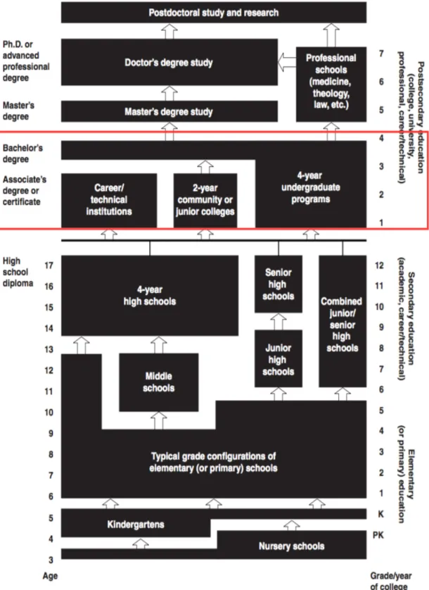
Before getting into the heart of the topic, we should clarify the framework in which U.S. students, especially U.S. college students, operate. Similar to the rest of the world, the U.S. education system is divided into three levels: (i) primary or elementary school, (ii) secondary school and (iii) postsecondary school. The Figure 1.1 provides the structure of education in the United States.

In Figure 1.1, we can see that students generally attend primary school from the age of six and spend 4 to 6 years in primary school. Before attending primary school, students may spend one to three years in pre-primary programs. Students normally spend 4 to 8 years in secondary schools depending on which primary grade is the final one and then complete secondary school following grade 12. Therefore, students attending an 8-year primary school only require 4 additional years of study to get a high school diploma while those who attend a 4-year primary school have to attend a middle school before attending a 4-year high school. Those who attend a 5-year primary school have to spend 7 years in secondary schools, whether

(25)

Figure 1.1 – The structure of education in the United States

Source: U.S. Department of Education, National Center for Education Statistics, Annual Reports Program through Snyder and Dillow(2015)

(26)

in junior high school followed by senior high school or in a combined junior/senior high school. The postsecondary education is also divided in two main levels: the undergraduate programs and the graduate programs. According toSnyder and Dillow(2015), the students who decide to attend graduates programs have to spend at least one year of coursework beyond the bachelor’s to complete a master’s degree and at least three years to complete a doctoral degree. As seen in Figure 1.1, professional schools are an alternative to graduate programs. Graduate programs include postdoctoral studies and research.

Our study is about undergraduate programs, generally called college (framed in Figure 1.1). There are two types of college: 4-year college and 2-year college. The 4-year college students represent more than the three-quarters of college students and usually spend 4 years to get a bachelor’s degree. They may later pursue graduate studies. There are also two kinds of 2-year college: 2-year community or junior colleges and career/technical institutions. "2-year colleges focus on associate degrees and various certification programs, which usually take only two years to attain and unlike four-year colleges they are required by law to accept everybody, and have much lower tuition costs than four-year schools"1_{. Unlike 4-year colleges, these}

2-year colleges do not have post-graduate programs available, however, according to Snyder and Dillow (2015), academic courses completed at a 2-year college are usually transferable for credit at a 4-year college in order to get a bachelor’s degree. According to them, a ca-reer/technical institution offers postsecondary technical training programs of varying lengths leading to a specific career.

Graduation requirements vary from institution to institution, but in all institutions, college students (all postsecondary students) must pass all compulsory courses in addition to a suf-ficient number of optional courses and must have an adequately high grade point average (GPA). This minimum grade varies from institution to institution and could vary from year to year; this pass grade is 2 in most colleges. "Grades out of 100% translate into a letter grading system. Passing grades are A for best, B for above satisfactory, C for just satisfac-tory, D for below satisfacsatisfac-tory, and F for failing [usually a grade of less than 50%], although some districts do not use the D grade. Pluses and minuses are used to show distinctions between grades. A student’s grades translate into a grade point average (GPA) according to a formula. By most systems, the highest GPA possible is a 4.02_{. GPAs are of great interest to}

colleges; they also determine class rank."3 _{To have the possibility to pursue graduate studies,}

the required GPA is greater than the pass grade and some specific courses could be required. 1

http://tvtropes.org/pmwiki/pmwiki.php/UsefulNotes/AmericanEducationalSystem

2_{corresponding to the passing grade A. The passing grade B is translated into a GPA of 3, the passing}

grade C is translated into a GPA of 2, the passing grade D (if it exists) is translated into a GPA of 1, and the failing grade of F is translated into a GPA of 0. These letters replaced the old grading system: E, S, M, I and F for E(xcellent), S(uperior), M(edium), I(nferior), F(ailing). Plus and minus notations respectively add and subtract 0.33 points except for the grade F. The passing grade A+ exists in a few institutions while the passing grades F+ and F- do not exist

3

(27)

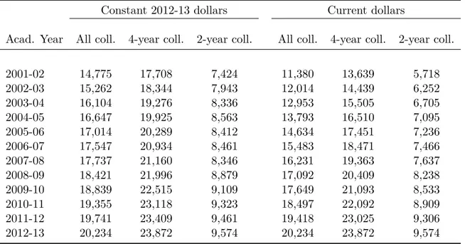
In addition to the grade requirement, students face another challenge: covering the costs of school fees and other costs in consideration of how doing so may influence their grades. The costs are enormous and have been growing fast for some time now. Table1.1provides average total tuition, fees, and room and board rates charged for full-time college students from the 2001-02 academic year to the 2012-13 academic year.

Table 1.1 – Average total tuition, fees, and room and board rates charged for full-time college students from the 2001-02 academic year to the 2012-13 academic year

Constant 2012-13 dollars Current dollars

Acad. Year All coll. 4-year coll. 2-year coll. All coll. 4-year coll. 2-year coll.

2001-02 14,775 17,708 7,424 11,380 13,639 5,718 2002-03 15,262 18,344 7,943 12,014 14,439 6,252 2003-04 16,104 19,276 8,336 12,953 15,505 6,705 2004-05 16,647 19,925 8,563 13,793 16,510 7,095 2005-06 17,014 20,289 8,412 14,634 17,451 7,236 2006-07 17,547 20,934 8,461 15,483 18,471 7,466 2007-08 17,737 21,160 8,346 16,231 19,363 7,637 2008-09 18,421 21,996 8,879 17,092 20,409 8,238 2009-10 18,839 22,515 9,109 17,649 21,093 8,533 2010-11 19,355 23,118 9,323 18,497 22,092 8,909 2011-12 19,741 23,409 9,461 19,418 23,025 9,306 2012-13 20,234 23,872 9,574 20,234 23,872 9,574

Note: constant dollars based on the consumer price index, as prepared by the Bureau of Labor Statistics,

U.S. Department of Labor, adjusted to a school-year basis.

Source: U.S. Department of Education, National Center for Education Statistics (2015). Digest of Education

Statistics, 2013 (NCES 2015-011), Table 330.10 through https://nces.ed.gov/fastfacts/display.asp?id=76

In Table1.1, we can see that, for the 2012-13 academic year, estimated total costs for tuition, fees, and room and board were $20,234 at college, $23,872 at 4-year college and $9,574 at 2-year college. For the 2000-01 academic year, average costs were $11,380 at college, $13,639 at 4-year college and $5,718 at 2-year college. Thus, in the 11 academic years between 2000-01 and 2012-13, costs rose 77.8% at college (5.4% annual rate), 75.0% at 4-year college (5.2% annual) and 67.4% at 2-year college (4.8% annually). After adjusting for inflation, over this 11-year period costs rose 36.9% at college (2.9% annually), 34.8% at 4-year college (2.8% annually) and 29.0% at 2-year college (2.3% annually). The huge difference between the costs of studies at 4-year college and 2-year college could be explained by the fact that for a 2-year program people will generally study in their hometown, can live at home, and so don’t have additional costs.

(28)

re-ceive many financial supports, ranging from their parents, the federal and state governments, private organizations, their college and various other sources of assistance. These financial supports could be parental transfers, parental loans, grants, scholarships, loans, work finan-cial study, employer assistance and other assistance.4 _{However, in most cases these financial}

supports are not sufficient to meet all of the costs. Therefore, students are obliged to work during the academic year. However, financial issues are not the only reason that students work during the academic year. Some students work in order to improve their living condi-tion. Nevertheless, there are a number of ways in which this employment could negatively impact academic performance. This chapter addresses how employment could affect aca-demic performance taking into account hours studied, which is not taken into account in the literature.

1.3 Data and descriptive statistics

1.3.1 Data

Our data comes from the National Longitudinal Survey of Youth 1997 (NLSY97) which is a part of the National Longitudinal Surveys (NLS) program. The NLSs, sponsored by the U.S. Bureau of Labor Statistics, are nationally representative surveys that follow the same sample of individuals from specific birth cohorts over time. The NLSY97 Cohort is a longitudinal project that follows the lives of a sample of 8,984 American youth born between 1980 and 1984. These respondents were aged 12-17 when first interviewed in 1997. This cohort of the NLSY is representative of the U.S. population born between 1980 and 1984. The number of respondents in the survey was 8,984 individuals initially with 4,599 (51%) males and 4,385 (49%) females interviewed in round 1 in 1997. About 83 percent (7,579) of individuals from the round 1 sample were interviewed in round 14 in 2010.5

To determine how employment during the academic year influences academic performance, we restrict our dataset to observations from the years 2000-2006, corresponding to the years when most of the individuals in the sample were in college. For each year between 2000 and 2006, we retain the individuals who attend college and had a grade point average (GPA). Our main variables are observed for each individual in their first terms in college for each academic year. We use the college GPA from the first terms in an academic year to indicate the academic performance. These GPAs ranged from 0 to 4 with an average value of 3.2 for students attending college between 2000 and 2006. The hours studied represent the average hours per week during the first term of the academic year that the student interacts with instructors, teaching assistants, or fellow students in a physical or on-line classroom. The hours worked represent the average hours per week that a respondent works at any job during the normal

4

The study of these financial supports is the subject of Chapter 3

5_This _information _about _NLSY _comes _from _{www.nlsinfo.org} _and _access _data _at

(29)

academic year. The normal academic year excludes the weeks in summer. We observe that an average of 80% of students attending college participate in the labor market each year and those who participate in the labor market worked an average of 19.6 hours per week.

Table 1.2 – Means and standard errors of different variables for youths attending college born between 1980 and 1984

Variable Mean Std. Err. [95% Conf. Interval]

GPA 3.168 0.007 3.153 3.182

Hours worked

Worked 0.799 - 0.790 0.808

Hours worked per week 15.683 0.167 15.356 16.009

Hours worked if working 19.640 0.180 19.287 19.992

Hours studied 14.797 0.083 14.634 14.961

Yearly non-labor income 1026.059 134.243 762.901 1289.217 College type 2-year college 0.247 - 0.236 0.258 4-year college 0.753 - 0.742 0.764 Gender Male 0.431 - 0.419 0.443 Female 0.569 - 0.557 0.581 Race Black 0.102 - 0.096 0.108 Hispanic 0.097 - 0.091 0.103 Mixed race 0.013 - 0.010 0.016 Non-Hispanic white 0.789 - 0.780 0.798 Region North-East 0.185 - 0.175 0.195 North-Central 0.290 - 0.279 0.302 South 0.311 - 0.299 0.322 West 0.211 - 0.201 0.222 Place of residence Rural 0.210 - 0.200 0.221 Urban 0.790 - 0.779 0.800

According to our dataset, during the timeframe covered about one-quarter of students at-tended 2-year college and the three-quarters atat-tended 4-year college. Female students com-prised 57% of our restricted dataset. 21% of students live in rural areas, 31% of students live in the south, while 19% live in the northeast. Students living in the north-central region and the west region respectively account for 29% to 21% of college students in the sample. We report that there is a difference in racial proportions between the initial overall sample and

(30)

our restricted dataset in Table 1.2. For example, Non-Hispanic white accounts for 52% in the sample, but they represent 79% of those who attended college on average in each year. Black and Hispanic students, which initially represent 26% and 21% are only 10.2% and 9.7% among those who attended the college on average in each year. The non-labor income is total monetary gains in a given year except for labor income and the gains related to the educa-tion such as grants, loans, etc. It includes the income from own farm business, own non-farm business, partnerships, professional practice, child support, interest and dividends from stocks or mutual funds, rental income, monetary gifts (other than allowance) from parents, public support sources, and other non labor income not related to education.

1.3.2 Descriptive statistics

This subsection analyzes the average variations of GPA, hours studied and hours worked as affected by hours studied, hours worked and different categories of student’s characteristics. Table1.3provides average values of student’s GPA, hours studied and hours worked, classified by the hours studied, the hours worked and other individual characteristics. In Table1.3, we report that students who do not work and those who work less than 20 hours per week spend more time studying than those who work more than 20 hours per week. On average, students who work less than 20 hours per week perform better than others. Their average GPA is 3.18. The students who do not work perform better than students who work more than 20 hours per week. We find that on average students who spend less than 10 hours per week studying spend much more time in the labor market than the others (22 hours per week compared to 14 hours per week). In Table 1.3, we also report a strong positive correlation between the hours studied and academic performance.

On average, students attending 4-year college have a higher GPA than those who attend 2-year college. They spend more hours studying and fewer hours in the labor market than students attending 2-year college. Similarly, on average, female students perform better than male students while they spend less time studying and more time in the labor market than male students. On average, students in the North-Central region have the highest GPA but not the most hours studied. They also work the most hours, on average. Students in the South region on average have the lowest GPA and the least hours studied. Students in the North-East region on average have the most hours studied and the least hours worked. We remark that there are no significant differences between the average hours worked of students in the different regions.

On average, the non-Hispanic white students perform better than the others. Their average GPA is 3.21. On average they spend more time studying than students of the other races except for mixed race students. The black students, with an average GPA of 2.92, have the lowest GPA, while the Hispanic students, with an average GPA of 3.10, spend more time in the labor market and less time studying on average. The section provides a description of

(31)

Table 1.3 – Average values of GPA, hours studied and hours worked by individual character-istics (standard errors in parentheses)

GPA Hours studied Hours worked

Hours worked

Not working 3.157 (0.015) 15.363 (0.160) 0.000 .. Work less than 20 hrs 3.178 (0.010) 15.712 (0.111) 9.901 (0.103) Work more than 20 hrs 3.154 (0.011) 13.619 (0.123) 32.183 (0.219)

Hours studied

Study less than 10 hrs 3.111 (0.019) 6.336 (0.062) 22.344 (0.462) Study between 10 and 20 hrs 3.166 (0.007) 14.950 (0.036) 14.433 (0.187) Study more than 20 hrs 3.248 (0.022) 28.685 (0.298) 14.554 (0.518)

College type 2-year college 3.079 (0.015) 13.344 (0.173) 22.072 (0.351) 4-year college 3.191 (0.007) 15.373 (0.080) 13.824 (0.186) Gender Male 3.103 (0.010) 15.157 (0.115) 15.091 (0.265) Female 3.218 (0.009) 14.703 (0.095) 16.222 (0.216) Region North-East 3.144 (0.014) 15.564 (0.184) 15.210 (0.427) North-Central 3.233 (0.012) 15.324 (0.135) 15.980 (0.332) South 3.114 (0.012) 14.308 (0.123) 15.760 (0.283) West 3.175 (0.015) 14.736 (0.169) 15.659 (0.347) Place of residence Urban 3.167 (0.007) 14.783 (0.083) 15.674 (0.186) Rural 3.161 (0.015) 15.404 (0.165) 15.820 (0.396) Race Black 2.920 (0.014) 14.336 (0.163) 15.619 (0.387) Hispanic 3.095 (0.016) 13.899 (0.216) 18.831 (0.443) Mixed-Race 2.995 (0.070) 16.000 (0.673) 13.183 (1.436) Non-Hispanic white 3.211 (0.008) 15.095 (0.087) 15.384 (0.200)

the overall average behavior, but it does not tell us how employment could affect academic performance. The next two sections describe the model used to analyze how employment could affect academic performance and present the econometric results.

1.4 Theoretical model

Let us define the student’s full production function (FPF) as a function which links their academic performance to their allocation of time between hours worked in the labor market, hours studied and leisure.

(32)

where p represents the academic performance, e the hours studied, h the hours worked, l the leisure time and ε the zero-mean error term such that

E(p) = ˜p(e, h, l)

The sum of these allocations is equal to the fixed time endowment T .

T = e + h + l

The more students devote time to studying the more they gain knowledge and their academic performance increases, so higher hours studied would directly contribute to higher academic performance, i.e. ∂˜p

∂e > 0. The hours studied are temporary and profitable investments

into academic performance. Students who occupy their leisure time with sports would be tired. However, sport activities help to keep the body fit and enable the brain to think faster during exams. In addition, leisure is generally considered as rest time, i.e. less fatigue and less stress. Good rest leads no doubt leads to an improved quality of academic work and contributes to improve academic performance, so generally ∂˜p

∂l > 0. Employment in

non-academically related activities are generally physical and stressing. They could also reduce the quantity than the quality of academic works, that would negatively impact academic performance. There are some jobs which are not physical and do not require any physical effort. Such employment would have no direct effect on the quality of academic work and academic performance.

Isolating leisure in the time constraint and substituting into the full production function (FPF), one obtains the student’s partial production function (PPF) as a function which relates their academic performance to their hours worked and their hours studied.

E(p) = ˜p(e, h, T − e − h) = p(e, h) (1.2) Since l = T − e − h, then an increase in the hours worked h leads to a reduction in hours studied e, leisure time l, or both. This paper estimates 1) the impact of an increase in hours worked on academic performance when the adjustment (in the time constraint) is only done by reducing leisure, i.e. when the hours studied are unchanged and 2) the impact on academic performance of an increase in hours worked when the adjustment (in the time constraint) is only done by reducing hours studied, i.e. when the leisure time is unchanged. From the equation of the partial production function (PPF)

E(p) = ˜p(e, h, T − e − h) = p(e, h) one has ∂p(e, h|e) ∂h = ∂˜p ∂h − ∂˜p ∂l (1.3) and ∂p(e, h|h) ∂e = ∂˜p ∂e − ∂˜p ∂l (1.4)

(33)

And also ∂p(e, h|e) ∂h − ∂p(e, h|h) ∂e = ∂˜p ∂h− ∂˜p ∂e = ∂p(e, h|l) ∂h (1.5)

When the adjustment is only done by leisure, the impact on academic performance of an increase in hours worked is given by ∂p(e, h|e)

∂h in equation (1.3) with

∂˜p

∂h being the direct

effect and ∂˜p

∂l being the indirect effect due to adjusting leisure. When the adjustment is only

done by hours studied, the impact of an increase in hours worked on academic performance is given by ∂p(e, h|e)

∂h −

∂p(e, h|h)

∂e in the equation (1.5) with

∂˜p

∂e the indirect effect due to

the adjustment of hours studied. Similarly, the impact of an increase in hours studied on academic performance when the adjustment is only done by leisure, is given by ∂p(e, h|h)

∂e in

equation (1.4). When the adjustment is only done by hours worked, the impact of an increase in hours studied on academic performance is given by ∂p(e, h|h)

∂e −

∂p(e, h|e)

∂h which is the

opposite of the impact on performance of an increase in hours worked when the adjustment is only done by hours studied. Thus, the partial production function (PPF) allows identification of the impacts of an increase in hours worked on academic performance when the adjustment (in the time constraint) is only done by hours studied and when the adjustment is only done by leisure. It also allows for identification of the impact of an increase in hours studied on academic performance when the adjustment is done by hours worked and when the adjustment is only done by leisure.

When the adjustment is only done through hours studied, the impact of an increase in hours worked on academic performance is negative because ∂˜p

∂h < 0 and

∂˜p

∂e > 0. Intuitively,

if students substitute hours studied for work, the quality and the quantity of the hours studied will be lower and thus the academic performance will also be decreased. When the adjustment is only done by leisure, the impact of an increase in hours studied on academic performance is positive i.e. ∂p(e, h|h)

∂e >0. The negative effect of the decrease in the quality

of academic works on academic performance due to the decrease in leisure time is much less important than the positive effect of the increase in the hours studied. The evaluation of the impact of an increase in hours worked on academic performance when the adjustment is only done by leisure ∂p(e, h|e)

∂h is the main object of this paper. If the direct effect

∂˜p

∂h

of employment on academic performance is assumed negative or null, then the impact of an increase in hours worked on academic performance when the adjustment is only done by leisure is negative, i.e. ∂p(e, h|e)

∂h <0 because

∂˜p

∂l >0. If the direct effect of employment on

academic performance is assumed to be positive, i.e. ∂˜p

∂h >0, then the impact

∂p(e, h|e)

∂h <0

on academic performance of an increase in hours worked when the adjustment is only done by leisure could be theoretically negative, null or positive. However, this expected effect on academic performance of an increase in the hours worked when the adjustment is only done by leisure is negative or null, i.e. ∂p(e, h|e)

(34)

on academic performance is assumed positive, it could not be greater than the direct effect of leisure on academic performance.

In most studies in the literature on the impact of hours worked on academic performance, the hours studied (and thus leisure) are ignored. Therefore, this variable is implicitly included in the error term. From the partial production function (PPF), one has

E(p|e, h) = p (e, h) We measure ∂E(p|e, h) ∂e = ∂p(e, h) ∂e ∂E(p|e, h) ∂h = ∂p(e, h) ∂h

while in the literature, they measure the effect of hours worked h unconditionally on hours studied e, i.e ∂E(p|h)

Thus, not accounting for hours studied is the source of a potentially important omitted variable bias. When the conditional expectation of performance in the partial production function (PPF) is linearly separable in hours worked and hours studied,

E(p|e, h) = m (e) + n (h) Our approach measures the following two derivatives

∂E(p|e, h) ∂e = ∂m(e) ∂e ∂E(p|e, h) ∂h = ∂n(h) ∂h

In the existing literature, the role played by hours spent studying is ignored. This implies E(p|h) = n (h) +

Z T −h−l

0

m(e) f (e|h) de

The last termRT −h−l

0 m(e) f (e|h) de enters the unobservable element of the model and causes

bias. The measured effect of hours worked in the mis-specified model is given by

∂E(p|h) ∂h = ∂n(h) ∂h − m(T − h − l) f (T − h − l|h) + Z T −h−l 0 m(e)∂f(e|h) ∂h de

(35)

We observe that the bias is decomposed into two terms. The first term of the previous equation captures the effect of hours worked on school performance, the object of interest. The last two terms capture bias. The second term captures the effects due to the reduction in the support of hours studied e associated with an increase in hours worked h. This term has a negative sign. The third and last term captures the substitution effect of a change in the conditional distribution of e due to an increase in hours worked h, holding the e fixed. This last term cannot have a sign a priori without restrictions on the distribution f (e|h). Hence, the effect of omitting hours studied is indeterminate.

Note that an Instrumental Variable strategy cannot control for bias resulting from the omis-sion of e from the model. Any variable that shifts h will be correlated with the biased term, because it is generally not possible to find a valid instrument that is correlated with hours worked but uncorrelated with hours studied. This suggests that most studies on the impact of hours worked on academic performance could be likely to be strongly biased.

1.5 Econometric model

1.5.1 Model description

We show that the partial production function (PPF) allows identification of the impact of an increase in hours worked on academic performance following adjustments. Thus, we define our econometric model from the partial production function (PPF): p = p(e, h) + ε. The model for a student i at the time t is given by :

p

it

= λ

0

+ λ

1

h

it

+ λ

2

e

it

+ γ

1

Z

1it

+ u

i

+ ε

it

, i = 1, ..., n ; t = t

0

, ..., T (1.6)

where p is the GPA of the student indicating academic performance, h is the hours worked, e is the hours studied, Z1 is a set of exogenous variables that explain the academic performance, ui is the individual specific effect, εit is the error term following a normal distribution, and

λ0, λ1, λ2and γ1 are parameters. The hours studied e and the hours worked h are endogenous

regressors because they are correlated with the error term εit. Therefore, an estimation with

ordinary least squares of equation (1.6) leads to biased estimators.

1.5.2 Consequences of ignoring instrumental variables and how to solve them

Because of the endogeneity of hours worked and hours studied, the OLS regressions provide biased estimators. Assume a simple model

(36)

one has E(βOLS) = β + E P iendoiεi P iendo2i !

Since the variable endo is a endogenous variable, i.e. E(endoiεi) 6= 0, the OLS estimator

is biased. The bias is positive if the correlation between the variable endo and the error term ε is positive. Since doing well in school frees up time for the student to work, good grades can lead to a decision to work while in school (Montmarquette et al. (2007)), and so the unobservable component of the academic performance is positively correlated with hours worked and negatively correlated with hours studied. Therefore, the estimators which ignore instrumental variables could overestimate the value of λ1in model1.6and could underestimate

the value of λ2 in model1.6. Stinebrickner and Stinebrickner(2003), in showing why the OLS

and instrumental variables (IV) estimators yield very different results, realize that the OLS estimator uses both the between-job variation in hours that is assumed by the IV estimator to be exogenous and the within-job variation in hours that is assumed by the IV estimator to be endogenous.

If λ1 in model 1.6is negative as in most cases, the overestimation leads to a smaller negative

effect. For example, DeSimone (2006) found that the OLS coefficient is roughly five times smaller than the GMM coefficient of an additional weekly work hour on current year GPA while this GMM coefficient is negative. If the overestimation due to ordinary regression is too high, the coefficients may even become positive. As for Stinebrickner and Stinebrickner (2003), it seems likely that both the actions of students and the actions of labor supervisors contribute to a situation in which highly motivated students work more hours. As for them, with respect to the former, highly motivated students would be willing to work more hours than other students. Nevertheless, OLS regressions do not isolate these facts into true effects. They found that OLS estimates of the effect of hours worked on academic performance for the subsample of students who were assigned to each particular job were all positive and were generally statistically significant and quantitatively large. Lillydahl (1990), using OLS to regress of GPA on the set of independent variables including instruments as independent variables, found that the coefficient of hours worked is positive.

The method of Instrumental Variables will take into account these facts and will provide consistent estimates if the instruments are well chosen. We use lagged values of hours worked

hit−1 and hours studied eit−1 as instruments of the hours worked h and hours studied e. It is

clear that there is a strong correlation between the hours worked in two consecutive periods, as well as the hours studied in two consecutive periods, while the observed variables from a previous year are not correlated with this present error term εit if the error term is not

auto-regressive. However, using panel data, in the presence of individual specific effects the only instrumentation is not sufficient to remove bias.