Topology optimization of electrostatic MEMS including stability constraints

(1)

U N I V E R S I T E D E L I E G E Aerospace and Mechanical Engineering Department

Topology Optimization of

Electrostatic MEMS Including

Stability Constraints

PhD Thesis Dissertation

submitted in partial fulfillment

of the requirements for the degree of

’Docteur en Sciences de l’Ing´

enieur’

by

Etienne Lemaire

Ing´

enieur Civil Electro-M´

ecanicien (A´

erospatiale)

(2)

Jean-Claude Golinval (President of the committee) Professor - University of Liège

Pierre Duysinx (Supervisor) Professor - University of Liège Eric Béchet

Professor - University of Liège Vincent Denoël

Professor - University of Liège Patrick Dular

Research Director F.R.S.-F.N.R.S. - University of Liège Tristan Gilet

Professor - University of Liège Fred van Keulen

Professor - Delft University of Technology (Netherlands) Véronique Rochus

PhD, MEMS Design Engineer - IMEC (Belgium) Ole Sigmund

(3)

Abstract

Among actuation techniques available for MEMS devices, electrostatic actuation is often used as it provides a short response time and is relatively easy to implement. However, these actuators possess a limit voltage called pull-in voltage beyond which they are unstable. The pull-in effect, can eventually damage the device since it can be impossible to separate the electrodes afterward. Consequently, pull-in phenomenon should be taken into account during the design process of electromechanical microdevices to ensure that it is avoided within utilization range. In this thesis, a topology optimization procedure which allows controlling pull-in phenomenon during the design process is developed.

A first approach is based on a simplified optimization problem where the optimization domain is separated from the electrical domain by a perfectly conducting material layer making the opti-mization domain purely mechanical. This assumption reduces the difficulty of the optiopti-mization problem as the location of the electrostatic forces is then independent from the design. However, it allows us to develop and validate a design function based on pull-in voltage in the framework of a topology optimization problem.

Nevertheless, in some applications, the developed pull-in voltage optimization procedure suffers from design oscillations that prevent from reaching solution. In order to solve this issue, we propose to investigate an alternative approach consisting in formulating a linear eigenproblem approximation for the nonlinear stability problem. The first eigenmode of the proposed stability eigenproblem corresponds to the actual pull-in mode while higher order modes allow estimat-ing upcomestimat-ing instability modes. By includestimat-ing several instability modes into a multiobjective formulation, it is possible to circumvent the oscillations encountered with pull-in voltage design function.

Next, the possibility to generalize the pull-in optimization problem by removing the separation between optimization and electrostatic domains is studied. Unlike the original method, the dielectric permittivity has then to depend on the pseudo-density like the Young Modulus to represent the different electrostatic behavior of void and solid. Additionally, in order to render perfect conducting behavior for the structural part of the optimization domain, a fictitious per-mittivity is also introduced into the material model. Difficulties caused by non-physical local instability modes could be solved by using a force filtering technique which removes electrostatic forces originating from numerical inaccuracies of the modeling method. Thanks to these im-provements, the optimization problem based on the pull-in design function can be generalized. As a result, the optimizer is able to adapt the electrostatic force distribution applied on the structure which leads to a higher efficiency of the optimal device.

In order to illustrate the interest of the pull-in voltage design function, the pull-in voltage optimization problem is merged with the electrostatic actuator optimization problem. In this new optimization problem, the pull-in voltage does not appear anymore in the objective function but in a constraint which prevents the pull-in voltage to decrease below a given minimal value. Firstly, the new optimization problem is compared to the basic electrostatic actuator design procedure on basis of a numerical application. The pull-in voltage constraint proved to be very useful since it prevents the pull-in voltage of the mechanism to decrease below the driving voltage during the optimization process. Finally, the effect of geometric nonlinearity modeling is also tested on numerical applications of our optimization procedure.

(4)

I gratefully acknowledge the project ARC MEMS, Action de Recherche Concertée 03/08-298 funded by the Communauté Française de Belgique, which supported part of this thesis.

I express sincere gratitude to my advisor Professor Pierre Duysinx for offering me the opportunity to work in his research group and to complete this thesis. Along these years, I could always count on his unwavering support, guidance, advice and cheerfulness. I also wish to thank him for all the time he spent reading and correcting this thesis. Many thanks also to the present and former colleagues from the Aerospace and Mechan-ical Engineering department, who guided me in my research, helped me in my teaching assistant work, took part to the correction of this manuscript, or simply participated to the excellent atmosphere. I am especially thankful to my former office mate Laurent Van Miegroet for pleasant fellowship along these years and to Véronique Rochus for all the support and advice about electromechanical modeling.

I am grateful to Professor Mathias Stolpe for welcoming me at the Department of Math-ematics of Technical University of Denmark during one month. This stay has been for me a chance to exchange many ideas with other members of the TopOpt group and a great source of inspiration for this thesis.

I would like to acknowledge Professors Eric Béchet, Vincent Denoël, Tristan Gilet, Jean-Claude Golinval, Fred van Keulen, Ole Sigmund, Research director Patrick Dular and Doctor Véronique Rochus for accepting to participate in the examination committee of this doctoral thesis.

Last but not least, I could not finish this thesis without the continuous support and encouragement from Julie, my parents, my sisters and my brother. They deserve more thanks than I can write.

(5)

Author Publications

Publication in refereed journal

• E. Lemaire, V. Rochus, J.-C. Golinval, and P. Duysinx. Microbeam pull-in

volt-age topology optimization including material deposition constraint. Computer Methods in Applied Mechanics and Engineering, 194:4040–4050, 2008.

Book chapter

• O. Brüls, E. Lemaire, P. Duysinx, and P. Eberhard. Optimization of multibody

systems and their structural components. In K. Arczewski, W. Blajer, J. Fraczek, and M. Wojtyra, editors, Multibody Dynamics, volume 23 of Computational

Meth-ods in Applied Sciences, pages 49–68. Springer Netherlands, 2011.

Publications in proceedings

• E. Lemaire, P. Duysinx, V. Rochus, and J.-C. Golinval. Improvement of pull-in

voltage of electromechanical microbeams using topology optimization. In

Pro-ceedings of the III European Conference on Computational Mechanics. June 2006. • E. Lemaire, V. Rochus, C. Fleury, J.-C. Golinval, and P. Duysinx. Topology

opti-mization of microbeams including layer deposition manufacturing constraints. In

Proceedings of the 7th World Congress on Structural and Multidisciplinary Opti-mization. 2007.

• O. Brüls, E. Lemaire, P. Eberhard, and P. Duysinx. Design of mechanism

com-ponents using topology optimization and flexible multibody simulation. In

Pro-ceedings of the 8th World Congress on Computational Mechanics. 2008.

• P. Duysinx, C. Fleury, L. Van Miegroet, E. Lemaire, O. Bruls, and M. Bruyneel.

Stress constrained topology and shape optimization: Specific character and large scale optimization algorithms. In Proceedings of the 8th World Congress on

Com-putational Mechanics. 2008.

• E. Lemaire, V. Rochus, J.-C. Golinval, and P. Duysinx. Electromechanical

mi-crodevice pull-in voltage maximization using topology optimization. In

Proceed-ings of the 8th. World Congress on Computational Mechanics. 2008.

• E. Lemaire, P. Duysinx, and V. Rochus. Multiphysic topology optimization of

electromechanical microdevices considering pull-in voltage using an electrostatic force filter. In Proceedings of the 8th World Congress on Structural and

(6)

model on local pull-in in electromechanical microdevices topology optimization. In PLATO-N International Workshop-Extended Abstracts. 2009.

• E. Lemaire, L. Van Miegroet, T. Schoonjans, P. Duysinx, and V. Rochus.

Mul-tiphysic topology optimization of electromechanical micro-actuators considering pull-in effect. In Proceedings of the IVth European Conference on Computational

Mechanics. 2010.

• V. Rochus, E. Lemaire, and C. Geuzaine. Dual approach for an accurate

esti-mation of pull-in voltage. In Proceedings of the IVth European Conference on

Computational Mechanics. 2010.

• E. Lemaire, L. Van Miegroet, V. Rochus, and P. Duysinx. Topology optimization

of electrostatic micro-actuators including electromechanical stability constraint. In Proceedings of the 5th International Conference on Advanced COmputational

Methods in ENgineering. 2011.

• E. Tromme, E. Lemaire, and P. Duysinx. Topology optimization of compliant

mechanisms: Application to vehicle suspensions. In Proceedings of the 5th

Inter-national Conference on Advanced COmputational Methods in ENgineering. 2011. • E. Lemaire, L. Van Miegroet, E. Tromme, L. Noël, and P. Duysinx.

Eigenprob-lem formulation for electromechanical microsystem pull-in voltage optimization. In Proceedings of the 10th World Congress on Structural and Multidisciplinary

(7)

List of symbols

Finite element formulation

KC Condensed tangent stiffness matrix

K′_C Condensed tangent stiffness matrix derivative with respect to the load variable

Kt Tangent stiffness matrix

Kϕϕ Electrostatic part of the tangent stiffness matrix

Kuu Mechanical part of the tangent stiffness matrix

K0_uu Mechanical contribution to mechanical part of the tangent stiffness matrix

ϕ Electric potential vector

fm Mechanical forces vector

fes Electrostatic forces vector

fext Generalized external forces vector

fint Generalized internal forces vector

q Generalized displacements vector

Qes Electric charges vector

r Residual forces vector

u Mechanical displacements vector

Material properties

ε Dielectric permitivitty

ε0 Void dielectric permitivitty 1

(14)

ρs Design material density

E Young modulus

Es Design material Young modulus

Emin Young modulus of the soft material used to represent void in topology

optimization

Miscellaneous

Veig Voltage at which the stability eigenproblem is formulated

Vpi,pred,k Predicted pull-in voltage associated with kth eigenvalue of the stability

eigenproblem

Optimization

v Structure volume upper bound

pε Permittivity penalty parameter (SIMP)

pE Young modulus penalty parameter (SIMP)

(15)

Chapter 1

Introduction

1.1 General context of the thesis

Nowadays, miniaturization is one of the keys to technology evolution. For about twenty years, industry is able to manufacture mechanical sensors and actuators smaller than one square millimeter. These devices are called MEMS (Micro ElectroMechanical Systems) because they combine electrical and mechanical components that can be as small as one micron. Some of the most famous applications of MEMS devices include: accelerometers or gyroscopes that can be found in almost all smart phones today or are used for ESP and ABS systems in vehicles, Digital Mirror Device chips for projection displays and pressure sensors for car tires. Size reduction enhances possibilities and allows lower costs, lower power consumption and better reliability. However, several challenges come with this downsizing.

At first we can think of manufacturing difficulties. To reach sub-millimetric sizes, me-chanical parts of the devices were initially built using manufacturing processes adapted from electronic industry like lithography techniques [68]. Since that time, microfabri-cation methods have evolved and specific manufacturing methods have been developed such as LIGA or micromolding [68]. As these processes are very different from the macroscopic ones, they lead to unusual manufacturing constraints. Nevertheless, a great advantage of MEMS manufacturing techniques is that they generally comply very well with batch manufacturing in order to reduce the devices price.

Secondly, with the downscaling of the mechanical structure, physical effects that are often neglected at macroscopic scale become significant in MEMS and vice versa. For instance, magnetic, electrostatic, and thermomechanical forces may be larger than grav-ity forces. This can be seen as an advantage, since these forces can be used in order to create deformation or vibration of a part of the microsystem structure. However, it makes the modeling of microsystems more difficult, as it leads to strong couplings between several physical fields.

Consequently, the tools classically used to design at macroscopic scale cannot be applied 3

(16)

directly for MEMS design. The modeling methods and the optimization techniques must be adapted in order to take microscale specificities into account. In the domain of modeling software, different types of coupling strategies have been developed in order to model the interactions between several physical fields. In parallel, several research studies have been considering the development of optimization procedures dedicated to MEMS design [1, 56, 99, 129]. Classical optimization methods have been intended for problems including one single physical field. They have to be adapted to take into account the strong interactions between the multiple physical fields. New design criteria must also be developed to include MEMS distinctive behaviors. In addition, the unusual manufacturing constraints of microfabrication processes should be introduced into the optimization problem.

1.2 Objectives of the thesis

The present thesis is dedicated to the development of an optimization procedure for electrostatic microactuators. In these microdevices, an input voltage is applied to the device to create electrostatic forces which, in turn, generate mechanical deformations. Consequently, there is a strong coupling between mechanical and electrostatic fields as a modification of the electrostatic forces involves a deformation of the structure and vice versa. As a result of the coupling, the behavior of electrostatic microactuators is nonlinear. This thesis resorts to existing finite element formulation available in Oofelie software [76] to treat the strongly coupled modeling problem.

Moreover, the nonlinearity of the electrostatic actuators leads to an unstable behavior: the pull-in effect. The pull-in effect is analogous to buckling behavior as it corresponds to a limit point on the equilibrium curve. This phenomenon appears if a voltage greater than the so called pull-in voltage is applied to the device. Beyond this critical voltage, the actuator collapses and its electrodes stick together, potentially resulting in a per-manent damage of the device. Clearly, the pull-in voltage is an important property of electrostatic actuators, which has to be considered during design. Therefore, including the pull-in voltage into the developed optimization procedure is a central objective of this thesis.

The optimization method selected for the present thesis is topology optimization based on homogenization approach. This technique offers several advantages over other opti-mization methods. Firstly, it is more general than sizing and shape optiopti-mization as it provides larger design freedom to the optimization. Secondly, its practical implemen-tation is less complex than the level set methods. Moreover, applications of topology optimization to MEMS systems design are available in literature and offer promising results [56,86,99,129].

The objective to establish a topology optimization procedure for electrostatic actuators able to control pull-in voltage has been divided in several sub-objectives:

(17)

1.3 Layout of the thesis 5

- First of all, we need to be able to evaluate the pull-in voltage of a device and to develop a sensitivity analysis procedure for pull-in voltage. As sensitivity analysis is performed at each optimization iteration, the developed tool has to be as efficient as possible.

- Secondly, the material model classically used in topology optimization has to be extended in order to include electrostatic material properties. The choice of the material model is critical. Since the electrostatic forces are design dependent loads, an unsuitable material model can lead to local instability modes and to a failure of the optimization process.

- Additionally, the possibility to include manufacturing constraints in the optimiza-tion problem has to be investigated. We will consider the implementaoptimiza-tion of a constraint related to material deposition manufacturing processes.

- Once, the pull-in design function is developed and tested, the initial objective can be achieved by inserting the pull-in function as a constraint into a classical actuator design problem (e.g. maximizing the output displacement for a given input voltage).

All modeling and sensitivity analysis procedures developed in this thesis have been implemented into the C++ _{software Oofelie while Conlin optimizer [}₄₁_{] has been used}

to solve the optimization problem.

1.3 Layout of the thesis

After this introductory chapter, the two following chapters are mainly focused on the review of literature. This review covers the topics common to several or all of the chap-ters of the thesis. Moreover, for topics specific to one chapter, the literature review is proposed in the corresponding chapter. Next, Chapters 4 to 7 present the developments achieved along this work. Each of these chapters includes numerical applications in order to illustrate and also to justify the developments.

The outline of the thesis is presented in Figure 1.1. In Chapter 2, different practical ap-plications of electrostatic actuation in MEMS are firstly presented. Then, the behavior of electrostatically actuated microsystems is studied and pull-in effect is explained on the basis of a simple model. Next, the existing modeling methods suited to microelec-tromechanical coupling simulation are reviewed. More specifically, the finite element framework used in the present thesis is summarized. Chapter 2 ends with the develop-ment of a path following algorithm able to compute the pull-in point. This procedure is the basis of the sensitivity analysis used in the pull-in voltage optimization.

The state of the art of optimization applied to microsystems is detailed in Chapter 3. At first, sizing, shape and topology optimization techniques usually used for single physic problem are described. Then, some of the existing extensions of optimization to

(18)

multiphysic microsystems are presented. Special attention is given to existing studies considering electrostatic actuation.

Using the essential modeling tools presented in Chapter 2 and the topology optimiza-tion method described in Chapter 3, we can start developing the pull-in voltage design function. For the development and the testing of the new design function, a basic opti-mization problem consisting in maximizing the pull-in voltage is considered. Moreover, in order to solve the difficulties one by one, we first make the assumption that the op-timization and the electrostatic domains are separated resulting in a purely mechanical optimization domain.

Starting from this simplified optimization problem, a first approach to maximize pull-in voltage is presented pull-in Chapter 4. In this approach we optimize the actual value of pull-in voltage as it can be computed by using the path following algorithm. The efficiency of the method is illustrated on numerical applications. Moreover, in the framework of the assumed separation between optimization and electrostatic domains, a manufacturing constraint is also proposed. This constraint aims at avoiding the creation of closed cavities in order to make the design easier to manufacture using a material layer deposition process.

Alternatively, instead of following the equilibrium curve up to the critical point, an approximation of the pull-in voltage can be determined by formulating a linear stability eigenproblem at some stable point of the equilibrium path. The development of this approximated approach is described in Chapter 5. Moreover, it is also possible to formulate an optimization problem on the basis of the resulting approximated pull-in voltage. The main advantage of this approach is that it avoids optimization oscillations that may happen in some applications if the actual value of pull-in voltage is optimized. The promising results from Chapters 4 and 5 lead us to consider the generalization of the pull-in maximization problem in Chapter 6. The generalized problem broad-ens the design freedom by removing the assumption of separation of the optimization and electrostatic domains. Hence, the optimization domain becomes electromechanical and the location of electrostatic forces becomes design dependent. The generalization first requires the development of a new material model including both electrostatic and mechanical material properties. During the development it comes out that the ap-proximated formulation proposed in Chapter 5 is unsuited to the generalization of the optimization problem. Therefore, only the approach from Chapter 4 is retained. Addi-tionally, difficulties related to artificial local instability modes have to be investigated and circumvented. Chapter 6 finalizes the development of the pull-in voltage design function.

Next, Chapter 7 proposes the development of an actuator design procedure for electro-static microsystems. At first, a classical actuator design formulation is considered. A numerical application shows that the optimization procedure may fail because of the pull-in effect. This situation can be avoided by including the developed pull-in voltage design function as a constraint into the actuator optimization problem. The new design

(19)

1.3 Layout of the thesis 7

constraint enables the optimization problem to achieve the convergence without trouble. To conclude this chapter, the influence of large displacement modeling is investigated. Finally, the conclusion of the thesis and the perspectives for future work are presented in Chapter 8.

....

Maximum pull-in voltage design

...

.

Electromechanical modeling and pull-in search tools

Chapter 2

. Optimization tools

Chapter 3 .

Simplified optimization problem .

.

Pull-in voltage design function Chapter 4

.

Eigenproblem approximation Chapter 5

.

Generalized optimization problem Chapter 6

.

Electrostatic actuator design Chapter 7

(20)

(21)

Chapter 2

Electromechanical modeling

2.1 Introduction

Electromechanical microsystems integrate mechanical components to electronic circuits to enhance sensing capabilities or to create microactuators. With the introduction of these mechanical parts comes the necessity to generate mechanical forces at microscale. However, because of the scale reduction, dominant forces in microsystems are not the same as at macroscopic scale. As described by Senturia [94], thermal expansion, elec-trostatic or piezoelectric forces have to be considered in microsystems and can be used as actuation forces. Moreover, it is not always possible to model separately the different physical phenomena that are involved in MEMS as there may be a strong interaction between them. Therefore dedicated tools have to be developed in order to model accu-rately the coupling between the physical fields.

In the scope of this work, devices using electrostatic forces are studied. The actuators used to generate electrostatic forces are in fact similar to capacitors. Basically, they are composed of two electrodes between which a voltage difference is applied. The generated electrostatic forces tend to bring the two electrodes closer. The displacement created by the electrostatic force can then be used in different ways as explained later.

This chapter is dedicated to the review of the behavior of electrostatically actuated MEMS and to a description of the methods used to model this behavior. As mentioned in the introduction chapter, these devices exhibit a strong coupling between electrostatic and mechanical physical fields. A consequence of this coupling is that the mechanical response to a voltage input is highly nonlinear and an unstable behavior is obtained if the input voltage exceeds a threshold called pull-in voltage. This instability, named pull-in effect, is very similar to buckling commonly known in mechanics. Indeed, alike pull-in, buckling appears when the mechanical load applied to a structure becomes greater than a limit value and results in a collapse (unstable behavior) of the structure. The description of pull-in effect is the topic of the third section of this chapter.

Because of their complex behavior, the modeling of electrostatically actuated microde-9

(22)

vices requires specific techniques. In the scope of this thesis, two main tools have been used. At first, the physical coupling between electrostatic and mechanical effects is taken into account by using a monolithic finite element formulation developed by Rochus [91]. The review of the finite element formulation is proposed in the fourth section of this chapter. Secondly, to handle the nonlinear and potentially unstable behavior of the model, a path following procedure has been developed. Based on the normal flow al-gorithm proposed by Ragon [85] the path following procedure is presented in the last section of this chapter.

2.2 Electrostatic microsystems

As already stated in the introduction section, several physical phenomena can be used to generate mechanical forces in MEMS. Piezoelectric, electromagnetic, electrostatic and thermal expansion forces are common. A review and a comparison of actuation principles used in MEMS are proposed by Bell et al. [13]. This study compares maximum output displacement, maximum output force and frequency range provided by each type of actuator. It comes out that there is no ultimate actuator, which surpasses all others but that every actuator possesses strong and weak points. For instance, electrostatic combdrive actuators provide larger frequency range than thermal expansion actuators but smaller output force. However, with respect to other actuation principles, electrostatic actuation has the advantage to be easier to implement in practice. Indeed, electrostatic actuation is compatible with cheap and well-tested MEMS manufacturing process as CMOS [108]. Moreover, it is characterized by a low power consumption. For these reasons, electrostatic actuation is very popular in MEMS devices. This section presents a few examples among others of microsystems in which electrostatic actuation is involved.

2.2.1 RF switches

One of the most common types of electrostatically actuated microsystems is radio fre-quency (RF) switches. These devices are part of a larger group of microsystems named RF MEMS that regroup all MEMS dedicated to radio frequency integrated circuits as switches, filters or variable capacitors for example. The domain of RF MEMS is very large as shown by the comprehensive description of RF MEMS done by Varadan in his book [114]. We will focus here on devices that are based on electrostatic actuation like RF switches.

Radio frequency switches are mainly seen in telecommunication devices for signal rout-ing or to adjust gain of amplifiers. This application covers a very wide frequency range starting from 1 MHz (AM band) and ending at 100 GHz (W band) so that different types of switch are used according to the actual working frequency. RF MEMS switches have two competitors, the first ones are the macroscale electromechanical switches and the second ones are the solid state switches. Because of their slow switching speed and low

(23)

2.2 Electrostatic microsystems 11

resonance frequency, macroscale electromechanical switches (as electromagnetic relays) can only be used in low speed applications. Classical solid state switches have a very short response time and can be used at higher switching speed. However they intro-duce too much loss and do not provide sufficient isolation1 when the signal frequency is higher than 1 GHz. RF MEMS possess some advantages and disadvantages over the two other switching techniques. Thanks to scale reduction, their switching speed is higher than their macroscale counterpart and can be of the magnitude of one microsec-ond [125]. However they are still slower than solid state switches where it can be as low as 3· 10−9 s (see [114]). Nevertheless RF MEMS provide lower insertion loss2and better isolation than solid state switch specifically when the signal frequency is higher than 1 GHz. Another advantage of RF MEMS switches is the very low amount of energy they consume.

A micrograph of a simple RF MEMS switch is presented in Figure 2.1. The principle of this device is very simple. When no voltage is applied to the gate, a small gap between the beam and the drain prevents the signal from passing from the source to the drain. If a voltage is applied to the gate, electrostatic force bends the beam down and the beam comes in contact with the drain to close the circuit. If they are very basic, these devices have one major drawback. Since there is a direct contact between the beam and the drain, an electric arc can happen when opening the switch.

Figure 2.1: Metal contacting switch micrograph [125].

The electric arc generated when opening the switch may be harmful for the microde-vice and reduces its reliability. Nevertheless, provided that the signal frequency is high enough, it is possible to avoid this problem by choosing another design. The microswitch presented in Figure 2.2 is different from the previous one as it integrates a layer of di-electric material on top of the drain electrode. This shunt switch design was originally proposed by Goldsmith at Texas Instrument [126]. The insulating layer acts as a spacer between the signal path and the drain (the metallic membrane) when the mobile elec-trode is down. This device works thanks to the capacitance variation between up-state and down-state. In down-state, the shorter distance between the signal path and the membrane leads to a higher capacitance than in up-state. The capacitance ratio can reach 100 depending on the geometry and material chosen. Provided that the input signal frequency is high enough (typically greater than 10 GHz), the signal is deviated

1_{Signal attenuation through the switch in blocking state.} 2_{Signal attenuation through the switch in passing state.}

(24)

from the ’signal path’ to the ’ground’ when the beam is down (high capacitance) while it is allowed to go through the switch when the beam is up. As there is no direct contact between the mobile electrode and the drain, electric arc appearance is avoided.

Figure 2.2: Capacitive coupling switch sketch and micrograph [125].

2.2.2 Microelectromechanical resonator

Like MEMS switches, microelectromechanical resonators are also introduced in radio frequency electronic circuits. Most of the time, they are used as band-pass filters which are made of several resonators coupled together. An example of such a filter coming from Ref. [115] is presented in Figure 2.3. The geometry of the system is more complex

Figure 2.3: Micrographs of a microelectromechanical filter.

than the previous one. The filter is composed of three oscillators serially coupled using beams (coupling beams). The left one (drive resonator) is excited by electrostatic forces generated on the combdrive electrodes by the input signal. The central resonator has no combdrive electrodes but linear electrodes are available to allow tuning of its resonance

(25)

frequency. On the right, the combdrives attached to the sense resonator convert its movement into the output signal. These combdrives act as variable capacitors when the sense resonator moves. The output signal is generated by the combination of the sensing resonator displacement and of a bias voltage applied to the moving part. As the central resonator, the two other ones also possess linear electrodes that can be used to adjust their individual resonance frequency. These additional electrodes are very useful to correct imperfections due to fabrication tolerances and other parasitic interferences. These devices also possess solid state and macroscopic electromechanical equivalents. However, their interest lies in the high quality factor they can achieve, their good temperature stability and aging properties [125]. Different designs exist depending on the frequency band targeted. The device presented in Figure 2.3 is designed for a central frequency of 300 kHz a band-pass width of 510 Hz and reaches a quality factor (Q factor) of 590. To reach higher central frequencies, beam resonators, square plate resonators and disk resonators have been developed. Using two mechanically coupled microbeams, Bannon (see [9] and Figure 2.4(a)) has been able to design a RF filter with a central frequency of 8 MHz and a quality factor reaching 435. Later, using corner-coupled square plate resonators, Demirci (see [31] and Figure 2.4(b)) created an RF MEMS filter characterized by a 70 MHz central frequency and a Q factor greater than 9000. Finally, a central frequency up to 200 MHz has been achieved using disk resonator (excited radially) by Li (see [58] and Figure 2.4(c)).

(a) RF filter by Bannon [9]. (b) RF filter by Demirci [31].

(c) RF filter by Li [58].

(26)

2.2.3 Microelectromechanical gyroscopes

Gyroscopes are sensors used to measure the rotation rate of an object. This is another field where MEMS are taking more and more importance so that comprehensive reviews have been proposed (see for instance [2, 127]). The development of microgyroscopes has started more than two decades ago and microdevices able to measure rotation rate around one or even two axes are now commercially available.

Most of MEMS gyroscopes use the same physical principle involving Coriolis effect to detect rotation. A mass suspended by springs is vibrating linearly or angularly using electrostatic or electromagnetic actuation. As a consequence, if the device is rotated around one of its sensing axis, a Coriolis force appears on the oscillating mass and modifies its trajectory with respect to the device reference axes. The trajectory modification of the oscillator can be detected electrostatically (capacitance measure) or sometimes by using piezoresistors.

In his book [2], Acar describes several microgyroscope designs. As an example, Fig-ure 2.5 presents some sketches and a micrograph of a simple MEMS gyroscope devel-oped by Mochida et al. [71]. As shown by the sketches, the mobile mass is excited in

x direction using the combdrive electrodes (Drive electrodes). A rotation of the

de-vice around z axis results then in an out-of-plane movement of the mobile mass. This rocking movement can be detected because of the capacitance modification using the electrode placed beneath the proof mass as indicated by the cross-section sketch.

(a) Gyroscope sketches. (b) Gyroscope micrograph.

Figure 2.5: Sketches and micrograph of a MEMS gyroscope [71].

2.2.4 Electrostatically actuated micromirrors

Optics is another domain where MEMS bring improvements and new possibilities. MOEMS (Micro OptoElectroMechanical Systems) is the name of this class of MEMS dedicated to optical applications. These microdevices can incorporate micromirrors, microlenses and optical wave guides. This section is focused on the presentation of

(27)

electrostatic micromirrors. The most famous application of micromirrors is the DMD (Digital Mirror Device) projection display by Texas Instrument [110]. The core of this display consists in a 2D array of tiltable micromirrors. Each mirror corresponds to a pixel of the image and can be turned ’on’ and ’off’ by using electrostatic actuation. The micromirrors are similar to the one presented in Figure 2.6(a). The electrodes placed beneath the mirror allow tilting the mirror around its suspension axis deflecting light towards or off the screen.

(a) Basic torsional micromirror sketch. (b) Functioning of a micromirror.

Figure 2.6: Tortional micromirror principle [130].

Basically, micromirrors used in DMD only need to achieve two discrete positions corre-sponding to ’on’ and ’off’ states. However, another concept for projection display is the scanning display [51]. In scanning displays, rather than using an array of micromirrors to create a complete image at once, the image is created by a light beam that covers the complete area by a scanning process as illustrated in Figure 2.6(b). The main ad-vantage of this technique is that only two mirrors are needed (one for each direction). Conversely to DMD these mirrors have to be able to cover continuously the complete range of tilting angle. Moreover, aside from display applications, scanning micromirrors are also used in bar code readers, confocal microscopes and laser printers to replace the classic galvanometric mirror scanners.

A scanning micromirror design developed by Ko et al. [51] is presented in Figure 2.7(a). In this design, the planar electrodes are replaced by vertical combdrives to increase actuation force. Conversely to the coplanar combdrives used in microresonator design in Figure 2.3, the two combs of vertical combdrives are here shifted vertically as illustrated in Figure 2.7(b). This vertical offset results in vertical electrostatic forces that generate a torsion moment and tilt the mirror. In Figure 2.7(a), the central circular part is the mirror itself. The mirror is supported by an oval frame upon which actuating combs are placed. With the micromirror they developed, Ko et al. [51] have been able to setup a laser scanning display. They use the micromirror for high frequency horizontal scanning while the vertical scan is performed by a galvanometric mirror.

More recently, a two-dimensional electrostatic microscanner design has been proposed by Chu and Hane [28]. In this system, the mirror is supported by a gimbal frame whose rotation axis is perpendicular to the mirror one. Consequently, the device can carry

(28)

(a) Eye-type scanning mirror by Ko et al. [51]. (b) Vertical combdrive by Wu et al. [122].

Figure 2.7: Example of a torsional micromirror design.

out both horizontal and vertical scanning and avoids the needs for a second scanning mirror.

2.2.5 Microlens optical scanner

Aside from mirrors, lenses are also included in MEMS. An application of microlenses is optical cross connection (OXC) into optical switches. Basically, the lenses are used to steer light between two optical fibers arrays in order to send light from each input fiber to the right output fiber. Of course, this task could be achieved by micromirrors as those presented in last section. Nevertheless, the availability of microlens scanners allows sparing one component since the light coming from input optical fibers needs in any case to be collimated by a lens. Moreover, microlens scanner can easily compensate for deviation of the fiber position and avoid costly accurate positioning of a passive lens. Concerning performances, optomechanical switches present longer switching time (of the order of one millisecond) compared to their electronic counterparts. However conversely to electronic switching, they do not introduce any bottleneck by requiring conversion of the light signal into an electronic signal and the bandwidth of the optical network is preserved (see Ref. [107]).

Kwon et al. [54] present a design of microlens scanner as the association of a microlens and a MEMS XY-stage (see Figure 2.8(a)). The XY-stage role is to perform biaxial translation of the microlens in a plane parallel to the substrate to achieve adequate positioning of the lens with respect to the light ray (perpendicular to the substrate). In the device proposed by Kwon et al. electrostatic actuation is used to achieve this goal. The XY-stage is equipped with four pairs of electrostatic actuators that allow translating the lens along both directions. This is illustrated in Figure 2.8(b) where a voltage is applied on black electrodes while gray electrodes are disabled to achieve biaxial displacement. The XY-stage developed by Kwon et al. is able to move the lens of more than 55 µm.

(29)

2.3 Insight of the behavior of the electrostatic actuator 17

(a) 3D view of the optical scanner. (b) Bidirectional actuation.

Figure 2.8: Two-dimensional optical scanner by Kwon et al. [54].

2.3 Insight of the behavior of the electrostatic actuator

As described in the previous section, electrostatic actuation is a convenient and efficient way to produce forces in microelectromechanical devices. However, the nonlinearity of the electrostatic force with respect to the gap separating electrodes results in phenom-ena such as the pull-in effect. Pull-in effect is related to an unstable behavior of the actuator when the voltage exceeds an upper limit value called the pull-in voltage. Phys-ically speaking, this effect is very similar to nonlinear buckling occurring in mechanical structures or to divergence of aeroelastic wings.

To explain the behavior of electrostatic actuators, let’s consider the simplified device represented in Figure 2.9. This capacitive system is made up of two parallels and rigid plates with the upper plate suspended by a linear spring of stiffness k and the lower plate fixed.

V

k

x

d

₀

Figure 2.9: Simplified electromechanical actuator.

If we assume the plates large enough so that side effects are negligible, the electrostatic force resulting from the application of a voltage difference V between the plates can be written [87], fes= ε0 2 AV2 (d0− x)2 , (2.1)

(30)

air), A is the capacitor surface, d0 the initial distance between the plates and x the displacement of the upper plate. Moreover, the restoring force from the spring is simply given by:

fr =−kx.

After applying the Newton’s second law and a few manipulation of the resulting equa-tion, we can obtain the following equilibrium equation giving the voltage as a function of the displacement: V = √ 2kx (d0− x)2 ε0A . (2.2)

Figure 2.10 plots the normalized equilibrium equation in the plane (x, V ). We can see that this curve possesses a maximum in terms of voltage for x = d0/3. This maximum corresponds to the pull-in voltage (Vpi) and no equilibrium position can be found for

a greater voltage. Using Eq. (2.2), we can compute the value of pull-in voltage by substituting x = d0/3: Vpi= √ 8kd3₀ 27ε0A . (2.3)

Figure 2.10: Normalized equilibrium curve of the simplified actuator.

By analogy with structural buckling, the pull-in voltage corresponds to a limit load. In practice, the application of an electric potential creates an electrostatic force, which tends to bring the electrodes closer. However, as the upper electrode goes down, the electrostatic force increases proportionally to the inverse of the squared gap (see equa-tion (2.1)). Consequently, at pull-in point, the linear spring cannot balance anymore the raising of the electrostatic force and the mobile electrode collapses toward the fixed one.

In addition, the pull-in point divides the equilibrium curve in two parts: a stable one (solid line in Figure 2.10) and an unstable one (dashed line in Figure 2.10). This stability

(31)

2.3 Insight of the behavior of the electrostatic actuator 19

inversion can be checked by computing the effective stiffness (i.e. tangent stiffness) along the equilibrium path (xe, Ve). The effective stiffness is simply obtained by computing

the derivative of the total force f = fes+ frapplied to the mobile electrode with respect

to its displacement. keff =− df dxe = k− ε0AV 2 e (d0− xe)3 = k− 2kxe d0− xe .

The influence of the applied voltage on the tangent stiffness is plotted in Figure 2.11. Starting from one (mechanical stiffness of the spring) when no voltage is applied, the normalized tangent stiffness decreases when the voltage grows. Eventually, the tangent stiffness vanishes when the pull-in voltage is applied and becomes negative if we proceed on the equilibrium curve. It results in an unstable equilibrium position at the pull-in point and for larger values of the displacement. This property can be used to detect the pull-in point.

Figure 2.11: Normalized tangent stiffness against displacement on equilibrium curve. Depending on the application, the pull-in effect may be desirable or undesirable. In-deed, we have seen in the last section that RF-switches rely on a collapse of the mobile electrode. Conversely, pull-in effect has to be avoided in some MOEMS, in RF-filters and in gyroscopes. In the later devices pull-in may result in contact of the combdrive electrodes but may also lead to a collapse of the proof mass on the substrate. Unnec-essary contact is usually avoided in MEMS since firstly it can create a short circuit and may damage the microsystem and secondly even if a dielectric layer is placed to prevent short circuit, it can be impossible to separate the electrodes from each other after pull-in in wet environment (see Ref. [113]). Therefore, pull-in is an important phe-nomenon that has to be taken into account during MEMS design and this is the reason why this thesis proposes to introduce pull-in voltage criteria into topology optimization of MEMS.

(32)

2.4 Electromechanical finite element formulation

The finite element method is used in this thesis to model the behavior of electrostatic microdevices. The results provided by the finite element analysis will then be the basis of the electrostatic microdevice topology optimization. However, several finite element formulations are available in the literature and the one that suits the best the problem has to be selected. For multiphysic problems, finite element methods can be classified into two categories, staggered methods and monolithic formulations.

Staggered methods are the simplest to develop. Indeed these methods use sequential and separated computation for each physical field of the analysis domain as illustrated in Figure 2.12. In this way, it is possible to use different software codes for each physical field and take advantage of existing software tools. Depending on the coupling type, several iterations are needed to reach equilibrium between every physical field.

.

Electrostatic problem. Mechanical problem

Figure 2.12: Staggered modeling procedure

However, staggered methods may lack convergence when the interactions between the physical domains increase. Therefore it is sometimes required to resort to the sec-ond class of methods: monolithic formulations. Monolithic formulations gather several physics into one single global problem so that the different physical fields are solved simultaneously. One disadvantage of monolithic approaches is that existing software tools cannot be used and a specific formulation has to be developed.

The choice of the modeling method to use for electromechanical microdevices is dis-cussed by Rochus et al. [91]. This paper shows that when approaching pull-in, staggered methods lack convergence while monolithic methods remain reliable. Moreover, as it is described later, the pull-in voltage sensitivity analysis needed by the optimization process requires an accurate knowledge of the pull-in conditions. This means that we have to be able to reach exactly pull-in point which is not possible with a sufficient accu-racy using staggered methods. Therefore, the electromechanical monolithic formulation developed by Rochus is used in this thesis.

2.4.1 Variational approach

In order to achieve an electromechanical monolithic formulation, Rochus et al. [91] start from the internal work by integrating over the domain the Gibbs energy density

(33)

2.4 Electromechanical finite element formulation 21 G defined as follow: G = 1 2S T_T₋ 1 2D T_{E .} _(2.4)

Each term of the Gibbs energy corresponds to a physical field of the problem. The first one takes into account the mechanical part of the energy with the product between the strain tensor S and the stress tensor T, while the second term represents the electrostatic energy contribution with D the electric displacement vector and E the electric field vector. These physical quantities are related by the constitutive laws where H denotes the elasticity tensor and ε the dielectric tensor.

{

T = H S,

D = εE.

The internal energy of the system is computed by integrating the Gibbs energy density from Eq. (2.4) over the whole electromechanical domain Ω.

Wint= 1 2 ∫ Ω STT− DTE dΩ =1 2 ∫ Ω STT dΩ | {z } Wm −1 2 ∫ Ω(u) DTE dΩ | {z } We . (2.5)

It is important to note here the difference between the mechanical energy Wm

integra-tion domain and the electrical energy We integration domain. Indeed, the mechanical

energy is integrated over the reference domain Ω using a classical Lagrangian formula-tion. Conversely, the electrostatic energy depends on the mechanical displacements u and has to be integrated over the deformed domain Ω (u). These different integration do-mains are described in Figure 2.13 for a simple analysis domain containing two different materials. The mechanical energy integration domain is represented in Figure 2.13(a). It corresponds to the undeformed configuration. Conversely, the electrostatic energy integration domain has to take the mechanical deformation presented in Figure 2.13(b) into account. Therefore, the electric integration domain is shown in Figure 2.13(c).

(a) Mechanical domain. (b) Mechanical deformations. (c) Electrical domain.

(34)

The unknowns of the problem are the mechanical displacements u and the electric potential ϕ. These fields are discretized on each node of the finite element mesh. These unknowns are linked to the strains and to the electric potential by the compatibility

relations: _   Sij = 1₂ ( ∂ui ∂xj + ∂uj ∂xi ) , E =−∇ϕ.

In addition, the boundary conditions of the problem are defined for each physical field (Fig. 2.13): { u = u over Γu, t = t over Γt, { ϕ = ϕ over Γϕ, d = d over Γd,

where t denotes the surface tractions, d the electric surface charges while Γu, Γt, Γϕand

Γd are the portions of the electromechanical domain boundary Γ where respectively u,

t, ϕ and d have prescribed values. These four parts verify the following relations:

Γu∪ Γt= Γ, Γϕ∪ Γd= Γ,

Γu∩ Γt=∅, Γϕ∩ Γd=∅.

The external energy can then be expressed as follow:

Wext= ∫ Ω uTf dΩ + ∫ Γt uTt dΓ− ∫ Ω ϕρ dΩ− ∫ Γd ϕd dΓ,

where f denotes the imposed body forces and ρ the prescribed volume charge density over domain Ω. Let us notice that in the chosen formulation the nodal electric charges are analogous to the mechanical forces.

Next, the virtual work principle is applied by perturbing the state variables u and ϕ by kinematically compatible virtual displacements δu and δϕ and by imposing that the resultant variations of the internal energy δWintand the external energy δWexthave to

be equal. One of the specific feature of this procedure lies into the computation of the internal electrostatic energy We (see Eq. (2.5)). Indeed, since the integration domain

of We depends on the displacements u it is also impacted by the virtual displacements

δu. This difficulty is circumvented by resorting to a variable substitution in order to

express the integral of the perturbed electrostatic energy over the unperturbed domain. The computational details are available in Ref. [91].

2.4.2 Tangent stiffness matrix

The application of the variational approach to Gibbs energy leads to a linearized equi-librium equation of the strongly coupled electromechanical problem in Eq. (2.6). In this equation appear: the tangent stiffness matrix Kt, the generalized displacements

(35)

2.4 Electromechanical finite element formulation 23

displacements are composed of both the nodal electric potentials ϕ and the nodal me-chanical displacements u while generalized forces are collecting the electric charges Qes

and the mechanical forces fm.

[ −∂2We ∂ϕ2 −∂ 2_W e ∂ϕ∂u −∂2_W e ∂u∂ϕ ∂2_W m ∂u2 − ∂ 2_W e ∂u2 ] | {z } Kt [ ∆ϕ ∆u ] | {z } ∆q = [ Kϕϕ Kϕu Kuϕ Kuu ] [ ∆ϕ ∆u ] = [ ∆Qes ∆fm ] | {z } ∆g . (2.6)

As suggested by Eq. (2.6), the tangent stiffness matrix can be split into four blocks. The first one, Kuu, links the mechanical displacements to mechanical forces. According

to the physical origin of the contributions to this block, we can write:

Kuu= K0uu+ K∗uu.

Beyond the classical mechanical energy contribution K0_uuthe usual mechanical stiffness,

Kuu includes also a contribution from electrical energy K∗uu. This later contribution

comes from the dependency of the electrical energy on mechanical displacements. The influence of the electrostatic effects on the mechanical stiffness has been pointed out in Section 2.3. Indeed, while studying the simplified electromechanical actuator, we have seen that the linearized stiffness decreases when the input voltage is increased.

Secondly, the off-diagonal terms of the matrix generate a coupling between mechanical and electrical unknowns. The origin of these terms is also the dependency of the electri-cal energy on mechanielectri-cal displacements. It is indeed clear that mechanielectri-cal displacement results in a modification of the electric charge distribution and that conversely, a vari-ation of the electric potential distribution modifies the electrostatic forces.

Finally, Kϕϕ is simply equal to the pure electrostatic problem stiffness matrix. This

comes from the fact that mechanical energy does not directly depend on the electric potential. Indeed, the displacements being fixed, a voltage modification leaves the mechanical energy unchanged (as far as piezoelectricity is ignored). Consequently, the only contribution to this last block comes from electrostatic energy.

2.4.3 Summary

The electromechanical coupling can be modeled using two different approaches: stag-gered or monolithic. The monolithic approach requires the development of specific finite element formulation but allows solving both physical fields at once. Moreover, within the monolithic finite element formulation, it is possible to write the linearized equilib-rium equations. The related tangent stiffness matrix exhibits coupling terms linking the two physical fields. The monolithic nature of the formulation as well as the knowl-edge of the tangent stiffness matrix are two important assets as they enable us to use very efficient solvers like numerical continuation procedure. This association results in an accurate computation of the pull-in configuration of the studied electromechanical systems.

(36)

2.5 Normal flow algorithm

The optimization methods developed in this thesis require the ability to follow precisely the equilibrium curve of a microelectromechanical device and to locate limit points of this curve. However, this task cannot be achieved by the classical Newton-Raphson algorithm that is widely used in nonlinear mechanics. Indeed, Newton-Raphson method computes the response of the system for a given load level (i.e. the voltage in the present case). Therefore, theoretically, it would only be possible to compute the stable part of the equilibrium curve. However in practice, as explained by Rochus et al. [91], it is hardly possible to compute the stable part of the equilibrium curve since convergence is poor close to pull-in voltage. Hence pull-in conditions cannot be determined accurately. Another option consists in resorting to path following algorithms. These methods are more sophisticated than Newton-Raphson procedure but allow following the equilibrium curve from rest position and enable passing singular points like pull-in point. Using this ability to compute the complete equilibrium curve (stable and unstable part) it is then possible to locate pull-in point accurately.

Path following methods differ from Newton-Raphson by the fact that the load parameter is considered as a variable of the problem and can be adjusted to restore equilibrium alike state variables of the system. With this extra variable the system owns n + 1 variable for n equations (the equilibrium equations). Consequently an additional constraint (i.e. equation) is needed in order to close the system.

The various path following methods differ mainly in the nature of this supplementary constraint. Riks-Wemper method (see Refs. [85, 119]) constrains consecutive points to lie on a plane. Crisfield method (see Refs. [30, 59, 91]), also known as Arc-length method, is similar but the constraint plane is replaced by a sphere centered on last converged point. Normal flow algorithm (see Refs. [1,85]) makes use of Moore-Penrose pseudoinverse to solve the n×(n + 1) system of equations, which can also be interpreted as a constraint as explained in what follows.

However, it is difficult to determine the most efficient among available path following methods. The performance of the algorithms is problem-specific and depends on the quality of the implementation. Nevertheless, the three methods cited previously have been compared by Ragon et al. [85] on the basis of a nonlinear buckling benchmark. They conclude that normal flow algorithm is more efficient and more robust than the two other methods in buckling problems. Later, Abdalla et al. [1] have successfully applied normal flow algorithm to trace the equilibrium curve of electromechanical microdevices models. That is for these reasons that we select normal flow algorithm in the present thesis.

2.5.1 Homotopy methods

The normal flow algorithm is part of homotopy methods group also called continuation

(37)

2.5 Normal flow algorithm 25

solve systems of nonlinear equations when a good estimate of the solution is unknown a priori. The mathematical aspects as well as various implementations of homotopy methods are described in text books by Allgower [5,6].

Originally, the problems targeted by homotopy methods are systems of N nonlinear equation in N variables that can be expressed in the general way:

f (x) = 0. (2.7)

f (x) can be considered as a mapping fromRN toRN. The standard procedure to solve this type of problem is to use a Newton-type algorithm. Starting from a point x0∈ RN we can compute the sequence xi inRN such that:

xi+1= xi− [Df (xi)]−1f (xi) ,

where [Df (xi)] stands for the Jacobian matrix of f (xi). If x is a solution of the

system of equations and if x0 is sufficiently close to this solution, the sequence {xi}

finally converges to x. However, choosing x0 close to x generally requires preliminary knowledge of the problem. Without this knowledge, Newton method often fails because poor starting points are chosen. One solution to overcome the problem is to define a homotopy function h :RN× R → RN such that:

{

h (x, 0) = f (x) ,

h (x, 1) = g (x) , (2.8)

where the function g : RN → RN has known zeros. Consequently, if we suppose that

x0 is one of the zeros of g, the point (x0, 1) will be a zero of h. The definition of the homotopy function in equation (2.8) leaves a lot of freedom on the actual mapping between the two functions. Amongst others, a commonly used homotopy is the convex homotopy:

h (z) = h (x, λ) = (1− λ) f (x) + λg (x) ,

where we introduce z = [x, λ] a vector from Rn+1 that will be used in the following because of its conciseness.

The idea of continuation method is to follow a curve c (s) :R → RN× R starting from (x0, 1) such that h (c (s)) = 0 along the curve. Under conditions on smoothness of h and on existence of a solution to Eq. (2.7) as discussed in the book by Allgower [6], the curve c leads to a point (x, 0) where x is a zero point of f .

Several methods have been developed to numerically follow the c (s) curve. In Ref. [6] Allgower classifies them into two groups: predictor-corrector methods and piecewise-linear methods. In predictor-corrector methods, the exact curve is approximately fol-lowed by a sequence of points. The gap between the points and the curve depends on the stopping criteria of the correction process. For piecewise-linear methods one follows exactly a piecewise linear curve that approximates the actual curve c (s).

(38)

2.5.2 Normal flow algorithm mathematical formulation

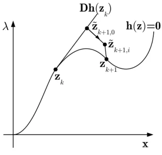
The normal flow algorithm belongs to the class of predictor-corrector methods. Fig-ure 2.14 summarizes the steps of a predictor-corrector iteration where the solid line represents the curve h (z) = 0. Starting from a known point on the curve zk, one first

tries to guess (or predict) the location of the next point zk+1of the curve. The prediction

˜

zk+1,0can be obtained tangentially or by using higher order information. The prediction

process is controlled by the progression step h, which is a measure of the distance

be-tween points zkand ˜zk+1,0. The value of h is usually chosen by the user and can possibly

be adapted by the algorithm to improve convergence properties. As the predicted point ˜

zk+1,0 does not usually lie on the curve, a correction phase is then applied to return on

the curve by computing a secondary sequence of points{˜zk+1,0, . . . , ˜zk+1,i, ˜zk+1,i+1. . .}

that converges towards zk+1.

Dh(z

_k

)

z

_k

z

_k+1

¸

x

z

_k+1,0

~

z

_k+1,i

~

h(z)=0

Figure 2.14: Predictor-corrector iteration with tangent prediction and correction pro-cess.

A simple approach for the prediction is to use a linear approximation of the curve

c (s), as it is classically done in Newton-Raphson method. The predicted point is then computed by moving of a distance h along the tangent to the curve. A more sophisticated approach is proposed by Watson [120] and implemented in the Hompack software package. Watson uses information from previous and current iterates (position and tangent vector) to define a Hermite cubic approximation of the followed curve c (s). If p (s) is the Hermite approximation constructed on the basis of points zk and zk−1

(whose curvilinear abscissa are respectively sk and sk−1), the next point on the curve

zk+1 is approximated as ˜zk+1,0 = p (sk+ h).

The correction process of the normal flow algorithm is analogous to the procedure used in Newton-Raphson method. However, since the homotopy function h (z) is a function