UNIVERSITÉ DU QUÉBEC À CHICOUTIMI
MÉMOIRE PRÉSENTÉ À L’UNIVERSITÉ DU QUÉBEC À CHICOUTIMI COMME EXIGENCE PARTIELLE DE LA MAÎTRISE EN RESSOURCES RENOUVELABLES
PAR
SAMUEL DUFOUR-PELLETIER B. SC. BIOLOGIE
MESURES COMPENSATOIRES POUR LA CONSERVATION DE LA FAUNE: ÉVALUATION DE L’EFFET DE LA SUPPLÉMENTATION DE BOIS MORT ET
DE CAVITÉS EN FORÊT BORÉALE AMÉNAGÉE
DÉPÔT FINAL JUILLET 2018
ii
RÉSUMÉ GÉNÉRAL
L’exploitation intensive des forêts peut réduire la disponibilité et la diversité de différents attributs associés aux vieilles forêts, tel le bois mort debout. Dans un contexte de conservation, il est possible de recréer artificiellement de telles structures et d’avoir un effet positif sur la faune associée. Cependant, ce type d’aménagement a été relativement peu étudié en forêt boréale de l’est de l’Amérique du Nord; particulièrement en ce qui a trait aux relations interspécifiques. Ce projet d’aménagement compensatoire a pour but de tester l’impact de la création artificielle de bois mort debout et de cavités en forêt boréale aménagée sur les coléoptères saproxyliques, les pics en alimentation ainsi que les utilisateurs secondaires de cavités, tout en mettant en relation diverses variables d’habitat à l’échelle locale et à l’échelle du paysage. Pour ce faire, nous avons provoqué la mort de 8000 épinettes noires par annelage du tronc selon deux distributions spatiales (uniforme ou groupés) et installé 450 nichoirs de 6 tailles différentes disposés soit à 0, 50 ou 100 mètres d’une bordure forestière. Pour tous les taxons d’insectes échantillonnés, nous avons capturé plus d’individus dans les sites avec création de bois mort que dans les sites témoins. Les marques d’alimentation présentes sur les arbres annelés nous permettent également d’affirmer que l’addition de chicots peut rapidement attirer les espèces de pics se nourrissant des insectes présents dans/sous l’écorce. Il semble également y avoir davantage de coléoptères saproxyliques et de marques d’alimentation de pics dans les traitements où le bois mort est groupé que dans ceux où il est distribué uniformément; cet effet n’est cependant pas statistiquement significatif pour les insectes. Le nombre de Curculionidae, de Cérambycidae et de Clearidae capturés varie en fonction des caractéristiques du paysage liées à la présence naturelle de bois mort (c.-à-d. coupes récentes, vieilles forêts, perturbations naturelles majeures et partielles), et ce à différentes échelles spatiales. Aucune de ces variables ne semble cependant influencer la présence de Scolytinés. La présence de marques d’alimentation de pics est quant à elle positivement associée à une plus grande proportion de coupes récentes 1 km autour des sites expérimentaux. La présence de ces marques est d’autant plus associée, à petite échelle, à des chicots morts récemment qui présentent un plus grand diamètre. Une année après leur installation, seulement 5 nichoirs ont été utilisés pour la nidification de mésanges à tête brune, et 19 ont été utilisés comme site de repos pour l’écureuil roux et/ou le grand polatouche. De surcroit, aucun changement global dans les populations d’oiseaux forestiers entre la saison de reproduction avant-aménagement et celle après-aménagement n’a été détectée. Les résultats obtenus nous permettent toutefois d’affirmer que de tels aménagements peuvent être bénéfiques très rapidement si le but premier est d’attirer les insectes saproxyliques associés au bois mort récent ainsi que leurs prédateurs. Pour la faune cavicole, il apparaît que d’autres facteurs limitent le degré et la rapidité de réponse à un apport anthropique en sites de nidification ou de repos. D’autres études seraient nécessaires afin de développer des méthodes favorisant l’implantation de ces mesures compensatoires dans un contexte commercial, et ainsi apporter des bénéfices à plus grande échelle.
iii
AVANT-PROPOS
Le présent mémoire a été réalisé dans le cadre du programme de maîtrise en Ressources Renouvelables de l’Université du Québec à Chicoutimi sous la direction du Pr Jacques Ibarzabal et la co-direction du Dr Junior A. Tremblay d’Environnement et Changements Climatiques Canada.
Ce projet a été principalement financé par le Programme de Financement de la Recherche
et Développement en Aménagement Forestier du Ministère des Ressources Naturelles du
Québec. Un soutien financier a également été fourni par l’Université du Québec à Chicoutimi. Le candidat à la maîtrise a également obtenu une bourse d’étude de la part de Protection des Oiseaux du Québec en 2015 et en 2016, ainsi qu’un soutien financier de la part du Centre d’Étude de la Forêt pour sa participation à un congrès international. La participation financière du Dr Thibault Lachat de la Haute École Spécialisée Bernoise a également permis de faire une analyse plus poussée de certains échantillons récoltés. La structure choisie est celle d’un manuscrit rédigé sous la forme d’un article scientifique en anglais qui sera soumis à la revue révisée par les pairs Forest Ecology and Management. Ce chapitre principal est accompagné d’une introduction et d’une conclusion générales en français.
Composition du comité évaluateur :
Annie Deslauriers, présidente du jury, Université du Québec à Chicoutimi Jacques Ibarzabal, directeur de recherche, Université du Québec à Chicoutimi Junior A. Tremblay, co-directeur de recherche, Environnement et Changements Climatiques Canada
iv
REMERCIEMENTS
De nombreuses personnes ont contribué, de diverses façons, à la réussite de mes études de deuxième cycle. Je tiens d’abord à remercier mon directeur de recherche Jacques Ibarzabal pour la confiance et la latitude qu’il a su me confier tout au long de ce projet. Cela m’a donné l’opportunité de m’épanouir dans tous les volets de mon parcours académique. Je remercie également mon co-directeur Junior A. Tremblay pour sa disponibilité implacable et ses judicieux conseils qui m’ont permis de rester motivé et concentré d’un bout à l’autre du processus. Grâce à votre expertise et votre passion, j’ai pu développer un intérêt profond pour l’ornithologie, et même, l’entomologie forestière!
Je dois également un énorme merci à tous mes proches, dont mes parents, qui ont su me soutenir à chaque étape. Malgré la distance, vos nombreux conseils ont décidément orienté pour le mieux plusieurs de mes décisions. Je dois une immense reconnaissance à ma conjointe Vanessa pour l’aide qu’elle m’a apportée à plusieurs reprises et à sa compréhension monumentale envers les nombreux « ouin, mais non…je dois travailler ». Peu de personnes accepteraient des journées entières de pluie battante en forêt à 4°C en guise de « week-end de couple ». Merci de nouveau à Jacques, ainsi qu’à mes collègues du Conseil des Abénakis d’Odanak, pour m’avoir permis de concilier travail-famille-étude pendant un peu plus d’un an.
Ce projet n’aurait pas pu être possible sans l’effort de nombreuses personnes sur le terrain. Merci à Joanie, Jérôme, Jean-Guy, Marie-Josée, Tommy, Karyane, Christophe, Michelle, Pascal, Émilie et Vanessa d’avoir participé à l’annelage de 8000 arbres et l’installation de 450 nichoirs sans même avoir bronché une seule fois. Votre enthousiasme indéfectible a contribué à ce que chaque moment passé sur le terrain fût un bon moment, et ce malgré les mouches.
Finalement je tiens à remercier André Desrochers et ses étudiants pour m’avoir accueilli dans leur laboratoire lors de ma première année d’étude ainsi qu’à Jean-Michel Béland et Christian Hébert pour le soutien apporté en lien avec le volet entomologique.
v
TABLE DES MATIÈRES
RÉSUMÉ GÉNÉRAL ... II AVANT-PROPOS ... III REMERCIEMENTS ... IV TABLE DES MATIÈRES ... V LISTE DES FIGURES DU CHAPITRE 1 ... VI LISTE DES TABLEAUX DU CHAPITRE 2 ... VI LISTE DES FIGURES DU CHAPITRE 2 ... VIII
CHAPITRE 1 : INTRODUCTION GÉNÉRALE... 1
CHAPITRE 2 : COMPENSATORY MEASURES FOR WILDLIFE CONSERVATION: TESTING THE EFFECT OF DEADWOOD AND CAVITY SUPPLY ON CAVITY USERS IN MANAGED BOREAL FOREST ... 9
Abstract ... 9 Introduction ... 10 Methods... 13 Results ... 25 Discussion ... 37 Acknowledgments... 48 Annexe ... 49 References ... 50
CHAPITRE 3 : CONCLUSION GÉNÉRALE ... 62
vi
LISTE DES FIGURES DU CHAPITRE 1
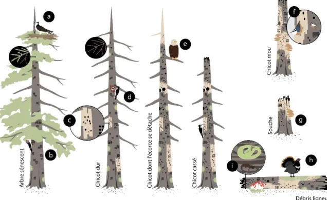
Figure 1. Exemples d’utilisateurs de différents types de bois mort en forêt boréale. a) Balbuzard pêcheur (Pandion haliaetus) nichant à la cime d’un vieil arbre, b) Pic maculé (Sphyrapicus varius) se nourrissant de sève, c) Insecte saproxyliques colonisant le bois, d) Pic à dos noir (Picoides arcticus) nichant dans sa cavité, e) Pygargue à tête blanche (Haliaeetus leucocephalus) utilisant un site de guet, f) Sitelle à poitrine rousse (Sitta canadensis) réutilisant une cavité, g) Champignon saprophyte décomposant le bois, h) Tétras du Canada (Falcipennis canadensis) sur un site de tambourinage, i) Amphibiens/reptiles utilisant les débris ligneux en état de décomposition avancé (adapté de Lang et al. 2015). ... 5
LISTE DES TABLEAUX DU CHAPITRE 2
Table 1. List and description of habitat variables. ... 20 Table 2. Codes for bird species. ... 24 Table 3. Interaction term of deadwood supply treatments and sampling year on the daily captures of saproxylic beetles from Type III Wald χ2 tests. ... 26 Table 4. Set of biologically relevant candidate models to predict the probability of presence of new foraging marks on girdled trees. ... 29 Table 5. Type III Wald χ2 tests for fixed effects on the probability of presence of new woodpecker foraging marks on girdled trees. ... 30 Table 6. Type III Wald χ2 tests for fixed effects on the probability of presence of new woodpecker foraging marks on girdled trees. ... 31 Figure 6. Projected probability of presence of new woodpecker foraging marks (± 95% CI) on girdled trees sampled in October 2016 based on the DBH of dead (black lines), dying (green lines) and live trees (grey lines) for a) uniform treatment and b) clustered treatment. ... 32 Table 7. Detection probabilities (p̂ ± SE) of birds (> 5 observations or counts) according to survey method (see Table 2 for species codes). ... 34 Table 8. Results of the RLQ analyses and comparison with the separate ordination analyses (R, L and Q alone) in June 2015 and 2016. ... 35
vii
LISTE DES FIGURES DU CHAPITRE 2
Figure 1. Map of the study area. ... 14 Figure 2. Visualization of the 6 experimental sites (i.e. every treatment combinations) within each experimental block (n = 5). ... 16 Figure 3. Mean capture (± SE) of Curculionidae, Cerambycidae, Cleridae and Scolytinae per day according to treatment and year. ... 27 Figure 4. Predicted probability (± SE; back-transformed from the logit scale) of presence of new woodpecker foraging marks on girdled trees during the three sampling seasons. 30 Figure 5. Projected probability of presence of new woodpecker foraging marks (± 95% CI) on girdled trees sampled in October 2015 (green lines), June 2016 (grey lines) and October 2016 (black lines) based on the proportion of recent cuts 1 km around sites for a) uniform treatment and b) clustered treatment. ... 31 Figure 6. Projected probability of presence of new woodpecker foraging marks (± 95% CI) on girdled trees sampled in October 2016 based on the DBH of dead (black lines), dying (green lines) and live trees (grey lines) for a) uniform treatment and b) clustered treatment. ... 32 Figure 7. RLQ scores of habitat variables (bold font and arrows; treatments are in red) and functional traits (squares = foraging strategy; black dots = nest location and type; white circles = migration strategy) for a) 2015 and b) 2016. ... 36
1
CHAPITRE 1 : INTRODUCTION GÉNÉRALE
Contexte généralL’entrée en vigueur de la Loi sur l’aménagement durable du territoire forestier (c. A-18.1, Gouvernement du Québec 2017) en avril 2013 a entraîné plusieurs nouvelles modalités de gestion de la ressource forestière au Québec. Ainsi, c’est en adoptant la Stratégie d’aménagement durable des forêts (SADF) que le nouveau régime forestier québécois vise, par le biais d’orientations et d’objectifs spécifiques, une gestion favorisant le maintien de la diversité biologique et la durabilité des écosystèmes (Ministère des Forêts de la Faune et des Parcs 2015).
L’exploitation forestière dans l’est de l’Amérique du Nord au cours des dernières décennies a causé un écart grandissant entre les paysages aménagés et naturels (Cyr et al. 2009; Boucher et al. 2016). Les écarts jugés les plus problématiques quant à leurs impacts potentiels sur les attributs écosystémiques (p.ex. structure et composition des peuplements, organisation spatiale) constituent alors des enjeux écologiques auxquels la SADF doit s’adresser (Grenon et al. 2010). Cette nouvelle démarche s’appuie donc plutôt sur des principes d’écologie forestière beaucoup plus inclusifs qu’une foresterie uniquement axée sur la récolte de la matière ligneuse (Gauthier et al. 2009).
Le concept établi afin de répondre aux cibles et objectifs de la SADF est l’aménagement écosystémique. Ce principe vise à diminuer l’écart entre la forêt naturelle et la forêt aménagée en s’inspirant, par exemple, de perturbations naturelles comme les feux de forêt, les épidémies d’insectes et les chablis. En respectant la plage de variabilité générée par les perturbations naturelles (c.-à-d. intervalle, taille, sévérité; voir Bergeron et al. 2007), on peut s’attendre à ce que les espèces de la forêt boréale soient plus susceptibles d’être résistantes et résilientes aux pratiques forestières, puisqu’on y conserve une gamme d’éléments auxquelles elles sont adaptées (Attiwill 1994; Landres et al. 1999; Drapeau et
al. 2016). Ainsi, c’est lors du processus de planification que les aménagistes ont recours à
des solutions concrètes afin d’appliquer les principes d’aménagement écosystémique et de bien prendre en considération les différents enjeux écologiques d’un territoire (Jetté et al. 2012a; Ministère des Forêts de la Faune et des Parcs 2014). La SADF stipule d’ailleurs que
2 les principaux enjeux écologiques au Québec sont, notamment, les changements dans la structure d’âge des forêts, la simplification de la structure interne des peuplements, ainsi que la raréfaction de certaines formes de bois mort (Ministère des Forêts de la Faune et des Parcs 2015).
Dynamique naturelle du bois mort en forêt boréale Québécoise
La forêt boréale continue de l’est de l’Amérique du Nord se classifie selon deux domaines bioclimatiques, soit la sapinière à bouleau blanc et la pessière à mousse, qui sont caractérisées par la nature de la végétation de fin de succession (Saucier et al. 2009). Les régimes de perturbations naturelles sont les principaux éléments conditionnant la structure et les fonctions écologiques des forêts (White et Pickett 1985; Franklin et al. 2002), et sont également à l’origine de la production de certaines formes de bois mort (Harmon et al. 1986; Franklin et al. 2007; Angers 2009).
En sapinière à bouleau blanc, ce sont principalement les épidémies d’insectes, dont la tordeuse des bourgeons de l’épinette (Choristoneura fumiferana), qui influencent la dynamique du bois mort (MacLean 1980; Morin et al. 2007). Les feux de forêt couvrent de petites superficies et cela permet généralement aux peuplements d’excéder la longévité des espèces d’arbres présentes (Gauthier et al. 2009). En pessière à mousse, ce sont les feux de grande envergure qui influencent majoritairement la disponibilité du bois mort tandis que les agents de perturbations secondaires agissent plutôt en toile de fond (De Grandpré et al. 2000; Harper et al. 2002; Pham et al. 2004). En effet, en l’absence de perturbations majeures dans ces deux domaines bioclimatiques, ce sont les épidémies légères, les chablis, les agents pathogènes ainsi que la sénescence naturelle qui assurent un apport relativement constant en bois mort, favorisant alors une structure forestière inéquienne (Desponts et al. 2004; Aakala et al. 2007; St-Denis et al. 2010). Bien qu’elles affectent de plus petites superficies, ces perturbations partielles façonnent tout de même la composition en bois mort de façon importante à l’échelle du paysage (McCarthy 2001). De plus, chaque arbre a le potentiel de passer par différents stades de décomposition suite à sa mort et ainsi de persister longtemps dans l’écosystème. Bien qu’il existe de nombreux systèmes de classification du bois mort (p.ex. Thomas 1979; Imbeau et Desrochers 2002), tous se basent sur l’aspect visuel de l’arbre (p.ex. présence et couleur du feuillage, présence
3 de brindilles et d’écorce, rupture de la cime, port de l’arbre) et sur la densité de la matière ligneuse (Angers et al. 2012a). Ainsi, la décomposition du bois peut s’amorcer dès la mort d’une branche ou de l’arbre entier, au stade sénescent ou chicot, et s’accélérer une fois tombé au sol, sous forme de débris ligneux (Yatskov et al. 2003; Angers et al. 2012a). De même, la quantité et le type de bois mort présent sur un territoire sont conjoncturels de nombreux facteurs, dont l’intensité et la prévalence des perturbations, le temps écoulé depuis la mort, ainsi que l’espèce d’arbre (Angers 2009). Par exemple, une épidémie ou un feu de grande intensité produira un fort apport momentané de bois mort (Nappi et al. 2011), tandis que des évènements de plus faible intensité entraineront une mortalité décalée dans le temps, qui se reflètera alors par des stades de dégradation variées (Vaillancourt 2008; Nappi et al. 2010). La dynamique de trouée, qui est omniprésente en vieille forêt boréale (Bergeron et al. 1998; Pham et al. 2004; St-Denis et al. 2010), assure également une disponibilité constante de tous les stades de décomposition de bois mort (Desponts et al. 2004; Aakala et al. 2008), en plus de favoriser la croissance des arbres, et donc de permettre la présence de gros chicots (Aakala et al. 2007; Vaillancourt et al. 2008).
En forêt boréale, les feuillus intolérants favorisent un développement rapide de structures de grandes tailles (p.ex. chicots, cavités naturelles, débris ligneux), puisque ces essences ont une croissance plus forte que les résineux et sont plus susceptibles d’être affectés par divers agents pathogènes (Darveau et Desrochers 2001; Martin et al. 2004; Angers 2009). Cependant, la présence de ces attributs ne permet pas de combler toutes les fonctions écologiques liées au bois mort en forêt boréale, car de nombreuses espèces dépendent plutôt du bois mort issu de résineux (Saint-Germain et al. 2007; Tremblay 2009). De plus, les chicots de feuillus se dégradent plus rapidement que ceux de résineux et ont ainsi un taux de chute plus élevé (Angers et al. 2010; Angers et al. 2012b). Par exemple, le temps médian entre la mort et la chute (c.-à-d. demi-vie) des chicots de peuplier faux-tremble (Populus tresmuloides) est d’environ 15 ans, tandis qu’il peut atteindre plus de 25 ans pour le pin gris (Pinus banksiana) (Angers et al. 2010). Chez l’épinette noire (Picea marianna) et le sapin baumier (Abies balsamea), la demi-vie est estimée à 18.1 et 19.5 ans respectivement (Angers et al. 2010), mais ces valeurs augmentent en fonction du diamètre des chicots (Aakala et al. 2008).
4
Rôle écologique du bois mort
Le bois mort remplit de nombreuses fonctions écologiques au sein de tous les écosystèmes forestiers mondiaux (Stokland et al. 2012; Seibold et al. 2015). Au Québec, il est documenté qu’un peu plus de 90 espèces de vertébrés utilisent le bois mort pour diverses fonctions et à certains moments de leur cycle de vie (p.ex. nidification, alimentation, repos; voir Lang et al. 2015). Bien que l’utilisation du bois mort par la faune aviaire soit généralement la plus documentée (Imbeau et Desrochers 2002; Drapeau et al. 2009; Ouellet-Lapointe et al. 2015), il n’en demeure pas moins que plusieurs espèces d’autres groupes taxonomiques, tels que les invertébrés (Saint-Germain et al. 2006; Seibold et al. 2016), les mammifères (Trudeau et al. 2011; Fauteux et al. 2012) et les amphibiens (Otto
et al. 2013; O'Donnell et al. 2014), sont étroitement associé à cette ressource. De plus, tant
en stade chicot que débris ligneux, plusieurs espèces de bryophytes, de lichens et de champignons saprophytes croissent directement sur le bois mort (Söderström 1988; Boddy 2001; Kushnevskaya et al. 2007).
La figure 1 schématise ainsi les rôles qu’un résineux peut avoir sur différentes espèces boréales en fonction des stades de décomposition du bois. Dès lors, plusieurs organismes interagissent entre eux à de multiples niveaux afin de former un ensemble complexe et interdépendant. Par exemple, en s’alimentant des insectes saproxyliques qui se développent dans le bois mort debout et en excavant des cavités de nidification, les pics vont favoriser la dispersion de champignons contribuant à la dégradation de la matière ligneuse (Jackson et Jackson 2004; Cockle et al. 2012). Ultimement, leurs cavités de nidification seront réutilisées par une foule d’autres espèces, dont certaines incapables d’excaver elles-mêmes leurs abris pour la nidification ou pour le repos (p.ex. Martin et Eadie 1999; Aitken et Martin 2007; Trudeau et al. 2012; Robles et Martin 2014). Une fois au sol, les conditions d’humidité et de températures des débris ligneux en état de décomposition avancée peuvent être plus stables que celles du substrat environnant, ce qui favorise alors la germination de certaines essences forestières et créer un habitat adéquat pour de nombreux amphibiens (Harmon et al. 1986; McGee et Birmingham 1997; Stevens 1997). Enfin, en se décomposant totalement, le bois mort joue un rôle majeur dans la séquestration du carbone par le sol et influence également la disponibilité des éléments nutritifs présents dans la litière forestière (Laiho et Prescott 2004; Wiebe et al. 2014; Strukelj et al. 2018). Tous ces
5 processus démontrent donc que les espèces dépendantes du bois mort se sont adaptées à traquer la disponibilité de cette ressource et à réagir continuellement aux variations temporelles et spatiales (Jonsson et al. 2005).
Figure 1. Exemples d’utilisateurs de différents types de bois mort en forêt boréale. a) Balbuzard pêcheur (Pandion haliaetus) nichant à la cime d’un vieil arbre, b) Pic maculé (Sphyrapicus varius) se nourrissant de sève, c) Insecte saproxyliques colonisant le bois, d) Pic à dos noir (Picoides arcticus) nichant dans sa cavité, e) Pygargue à tête blanche (Haliaeetus leucocephalus) utilisant un site de guet, f) Sitelle à poitrine rousse (Sitta
canadensis) réutilisant une cavité, g) Champignon saprophyte décomposant le bois, h)
Tétras du Canada (Falcipennis canadensis) sur un site de tambourinage, i) Amphibiens/reptiles utilisant les débris ligneux en état de décomposition avancé (adapté de Lang et al. 2015).
Enjeux écologiques liés au bois mort
Dans plusieurs écosystèmes mondiaux, il a été démontré que la diversité et la quantité de bois mort tendent à diminuer en raison de nombreux facteurs anthropiques (Siitonen 2001; Bouget et al. 2012; Lindenmayer et al. 2012). À titre d’exemple, plusieurs décennies de foresterie intensive ont entrainé une diminution importante de la quantité et de la diversité
6 de bois mort au sein des forêts boréales Fennoscandinaves (Östlund et al. 1997; Linder et Östlund 1998; Siitonen 2001). Hekkala et al. (2016) résument d’ailleurs qu’il y a approximativement 5 à 7 m3/ha de bois mort total dans les paysages aménagés, tandis que les forêts naturelles en comprennent entre 60 et 120 m3/ha. Cette limitation de la ressource a ainsi contribué au déclin à grande échelle de nombreuses espèces associées au bois mort (Berg et al. 1994; Rassi et al. 2010).
Au Québec, bien que la situation générale soit moins dramatique qu’en fennoscandinavie, il est possible d’observer localement certains écarts dans les quantités de bois mort en lien avec l’aménagement forestier (Angers 2009; Côté et al. 2009). À cet égard, Tremblay et
al. (2009) ont rapporté qu’une vieille pessière à mousse naturelle (>90 ans) comptait en
moyenne 71,3 m3/ha de bois mort total et que cette valeur diminuait à 29,7 et 18,1 m3/ha respectivement dans les parterres de coupes récents (<5 ans) et les peuplements dénudés. Même si une comparaison directe entre les valeurs de bois mort observées dans les forêts fennoscandinaves et canadiennes ferait l’objet d’une étude en soit, les similitudes entre les deux milieux (p.ex. structure forestière, structure des populations d’oiseaux) rappellent qu’une foresterie intensive pourrait possiblement mener à des problèmes de conservation pour de nombreuses espèces locales associées au bois mort (Imbeau et al. 2001).
En effet, plusieurs facteurs inhérents à l’exploitation des forêts boréales limitent la disponibilité et le recrutement du bois mort (Gauthier et al. 2009). Dans les forêts équiennes matures, la récolte est souvent totale et la longueur des révolutions ne permet généralement pas la croissance d’arbres de fort diamètre en plus d’annuler la mortalité par sénescence (Desponts et al. 2002; Desponts et al. 2004; Roberge et Desrochers 2004). De plus, même si d’importantes superficies touchées par des feux ou des épidémies sont laissées intactes, les coupes de récupération de certains secteurs suite à une perturbation naturelle peuvent localement empêcher un apport massif de bois mort (Nappi et al. 2004; Nappi et al. 2011). Enfin, lors des interventions sylvicoles, le bois mort déjà présent est souvent éliminé par mesure de sécurité pour les travailleurs ou écrasé par la machinerie.
7
Pertinence de l’étude et objectifs généraux.
Dans certains contextes, l’aménagement compensatoire de l’habitat peut être utilisée afin de pallier à une problématique ciblée, ou tout simplement comme outil favorisant le développement durable d’un territoire (Morris et al. 2006). Ce concept vise à contrebalancer les effets négatifs d’un impact anthropique (p.ex. foresterie, urbanisation, secteur minier) en restaurant artificiellement certains éléments clés de l’habitat dans le but d’y rétablir des fonctions écologiques ciblées. En forêt boréale, les écarts grandissants entre les paysages naturels et aménagés peuvent donc localement entraîner des situations où le recours à de telles mesures peut être envisageable. Dans le cas du bois mort, il a été démontré que la création artificielle est possible afin d’obtenir un effet positif sur de nombreuses espèces associées (p.ex. Hane et al. 2012; Kilgo et Vukovich 2014; Ranius et al. 2014; Barry et al. 2017).
Diverses techniques ont été élaborées afin de créer des chicots ou de simuler certains attributs structuraux liés vieilles forêts. Certaines études ont eu recours au dynamitage (Bull et Partridge 1986), aux souches hautes (Ranius et al. 2014), à l’inoculation de champignons par arme à feu (Filip et al. 2004), au brûlage contrôlé (Toivanen et Kotiaho 2010) ou à l’installation de nichoirs (Aitken et Martin 2012). Le choix de la méthode peut évidemment dépendre de nombreux facteurs, dont le type et la quantité de bois mort nécessaire, les restrictions logistiques et les espèces visées. À titre d’exemple, l’annelage manuel des arbres permet de créer du bois mort qui restera sur pied relativement longtemps (Hallett et al. 2001), mais nécessite d’importantes ressources en terme de main-d’œuvre. En contrepartie, l’étêtage des arbres peut se faire plus rapidement à l’aide de machinerie forestière, mais puisqu’un tronc brisé peut être une porte d’entrée importante pour certains agents pathogènes, ce type de bois mort se décomposera plus rapidement (Weiss et al. 2018).
Bien que ces techniques aient largement été utilisées dans des contextes où la faible disponibilité du bois mort menace déjà la conservation d’espèces y étant associées (p.ex. Fennoscandinavie), peu d’études ont été menées dans les forêts boréales de l’est de l’Amérique du Nord (Boucher et al. 2012; Gagnon 2013; Thibault et Moreau 2016). Toutefois, la majorité des études orientent leurs recherches sur des espèces ou des groupes
8 d’utilisateurs précis (p.ex. uniquement les insectes), ce qui limite l’étendue de l’interprétation en regard aux mécanismes écologiques interspécifiques (Seibold et al. 2015). Enfin, un nombre très limité d’aménagements compensatoires testent simultanément l’impact de différents types ou attributs de bois mort sur un même territoire (e.g. bois mort récent et cavités, Caine et Marion 1999).
Le présent projet contribue à combler ces lacunes en testant l’effet combiné de la supplémentation de bois mort debout et de cavités artificielles dans des peuplements forestiers d’épinettes noires de 50-70 ans sur deux grands groupes d’utilisateurs, soit les coléoptères saproxyliques et les vertébrés cavicoles (mammifères et oiseaux). Il est donc attendu que la supplémentation de chicots par annelage aura un effet positif sur les utilisateurs de bois mort récents tandis que l’addition de nichoirs permettra la nidification et le repos de certaines espèces cavicoles. À notre connaissance, il s’agit de la première expérimentation à grande échelle mettant en relation ces deux facteurs.
Les résultats de cette étude fourniront des pistes afin de déterminer si, dans un contexte où un problème de conservation relié au bois mort debout est identifié localement, il est possible d’agir rapidement et de rétablir les fonctions écologiques d’un territoire donné. Les connaissances acquises apporteront également des éléments supplémentaires pour les aménagistes afin d’adapter des méthodes représentatives des particularités régionales et logistiques. Ultimement, de telles méthodes pourraient en favoriser l’intégration dans des pratiques commerciales selon les principes de l’aménagement écosystémique.
9
CHAPITRE 2 : COMPENSATORY MEASURES FOR WILDLIFE
CONSERVATION: TESTING THE EFFECT OF DEADWOOD AND
CAVITY SUPPLY ON CAVITY USERS IN MANAGED BOREAL FOREST
Dufour-Pelletier, Samuel. Université du Québec à Chicoutimi
Tremblay,Junior A. Environnement et Changements Climatiques Canada Ibarzabal, Jacques. Université du Québec à Chicoutimi
Abstract
In managed boreal forests, where clearcuttings tend to induce a change in the amount and diversity of standing deadwood, it is possible to simulate old-growth forest attributes to have positive effects on deadwood associated species. This study evaluates the short-term response of saproxylic beetles, foraging woodpeckers and secondary cavity users to snag and cavity supply in 50-70 years-old black spruce stands. In spring 2015, 8,000 black spruces have been girdled according to two spatial distributions (uniform and clustered treatments) and 450 nest boxes of 6 sizes have been disposed at 3 different distances from a forest edge. In late-spring 2015 and 2016, there was a significantly higher number of beetles captured at snag supply sites than at control sites as well as a general trend to capture more beetles in clustered treatments than in uniform treatments. We captured approximately 7-fold less beetles in 2016 (1 year after girdling) than in 2015 (few weeks after girdling). Very few woodpeckers foraging marks were observed in October 2015 (6 months after girdling) and in June 2016 (1 year after girdling), but in return, a large amount of foraging marks was detected in October 2016 (1 year and a half after girdling). Woodpecker foraged significantly more on girdled trees in clustered treatments than in uniform treatments and preferred bigger and recently dead girdled trees rather than live or dying girdled trees. Depending on the insect taxa analyzed, we found that various habitat variables at different scales influenced the number of beetles captured. Similarly, woodpeckers foraging mark presence was positively associated with the proportion of recent cuts (≤ 10 years) 1 km around sites. Only 5 Boreal chickadee pairs used nest boxes and occupied the two smaller box sizes located away from the forest edge. Our study failed to detect global changes within the forest bird community structure. Nevertheless, our study showed that structural enrichment as a compensatory measure could be an effective way to rapidly attract deadwood associated species within non-optimal forest stands. Further studies in eastern Canadian boreal forests should aim to develop more adaptive methods to facilitate their implementation in commercial activities and thus favor benefits at larger scales; especially where forest structures have been locally driven outside of their range of natural variability and that a conservation concern is identified.
10
Introduction
In boreal ecosystems, it is recognized that forest management decreases the proportion of old-growth stands (Östlund et al. 1997; Boucher et al. 2009; Cyr et al. 2009), and consequently, induces changes in the amount and diversity of standing deadwood (Fridman and Walheim 2000; Roberge and Desrochers 2004; Vaillancourt et al. 2008). Indeed, time interval between clearcutting rotations does not allow the development of deadwood structures similar to those observed in old-growth forests (Drapeau et al. 2009). In most accessible territories, salvage logging after a natural perturbation also limits the recruitment of large areas of deadwood (Nappi et al. 2004). It has been shown that forest management have already induced changes in the overall landscape and age structure of eastern Canadian forests (Cyr et al. 2009; Bouchard and Pothier 2011; Boucher et al. 2015), and that management and conservation targets implemented over the past few decades have proven to be insufficient to prevent habitat loss below minimum ecological thresholds (Imbeau et al. 2015). As a comparison, several plant, animal and fungus species in Fennoscandia are now threatened by the loss of old-growth forest attributes due to several decades of intensive forestry (Berg et al. 1994; Siitonen 2001, 2012). Given the similarities between Fennoscandian and northeastern Canadian boreal forests (e.g. forest-age structure, structure of bird assemblages; Imbeau et al. 2001), it is imperative to develop further tools to limit possibilities of such an outcome.
Ecosystem-based forest management has emerged as a possible solution to reduce the negative effects of forestry on ecosystem properties (Bergeron et al. 2007; Gauthier et al. 2009). By emulating the pattern of natural disturbances (e.g. wildfires, insect outbreaks, windthrows), one can assume that a smaller gap between natural and managed forest would help to maintain forest structures inside their historical range of natural variability to which animals are adapted (Harvey et al. 2002). Forestry practices aiming to increase the diversity of the internal structure of forest stands and to promote the availability of different types of deadwood could be an asset for the conservation of deadwood associated species (Drapeau et al. 2009; Boucher et al. 2016; Ibarra et al. 2017).
Many vertebrates and insects rely on standing deadwood (hereafter snags) at some part of their life cycle (Speight 1989; Siitonen 2001; Stokland et al. 2012), and those associations
11 may differ from the type of deadwood produced. For instance, several saproxylic beetles are closely associated to specific habitat features (e.g. wildfires, Nappi et al. 2010), while other boreal species might be more opportunistic and rather forage or breed in unburned snags (Boucher et al. 2012). By digging galleries in the bark or the sapwood of recently dead trees, some aggregative beetles such as scolytids (Curculionidae) have a crucial effect on the dynamic of other species that use snags as foraging substrate (Murphy and Lehnhausen 1998; Drapeau et al. 2009; Edworthy et al. 2011). Indeed, some species such as the Black-backed (Picoides arcticus) and the American Three-toed (P. dorsalis) woodpeckers would prefer to forage on dying or recently dead trees rather than advanced-decay snags (Nappi et al. 2015; Tremblay et al. 2010, 2016; Cadieux and Drapeau 2017). Woodpeckers (primary cavity nesters), which also rely on snags to excavate cavities for nesting, are considered as keystone species in boreal ecosystems (Ouellet-Lapointe et al. 2015). Ultimately, woodpecker cavities will be used by many secondary cavity nesters/users – species unable to excavate themselves their shelter for nesting or roosting (Aitken and Martin 2007; Robles and Martin 2014). Other species such as chickadees and nuthatches (weak cavity excavators) frequently use existing cavities, but can create their own in well-decayed wood (Martin and Eadie 1999). Associations within nestwebs also depend on bird size, where large-bodied primary excavators would produce adequate cavities for larger secondary users such as owls and ducks (Martin et al. 2004). Furthermore, while feeding (i.e. by lifting the bark or pecking the wood), excavating or exploring, cavity users would favor the dispersal of wood decaying fungi, which will accelerate the decomposition rate of deadwood and provide further opportunities for species associated with highly decayed snags (Jackson and Jackson 2004; Cockle et al. 2012). Ultimately, fallen snags (coarse woody debris) would produce ideal habitat for many other organisms (see Stokland et al. 2012) and also have major implications for soil C sequestration and nutrient availability (Strukelj et al. 2018).
Some silvicultural practices, such as partial harvesting (Santaniello et al. 2017) or retention of both live and dead large trees in riverine and remnant linear forests (Remm et al. 2006; Vaillancourt et al. 2008) can allow a relative intake of deadwood at the landscape scale (Moussaoui et al. 2016). Nevertheless, those techniques are not always implemented in management strategies due to several economic or logistical restrictions, thus leading to a
12 possible local lack of old-growth forest attributes (Angers 2009). In that context, artificial supply of snags could have positive effects on associated wildlife (Hane et al. 2012; Seibold et al. 2015; Thibault and Moreau 2016a). In other boreal ecosystems, is has been shown that high stump creation and tree girdling provide suitable habitat for saproxylic beetles (Ranius et al. 2014; Thibault et Moreau 2016a), and that tree topping favors foraging and nesting of primary cavity nesters (Barry et al. 2017). Is it also possible to enhance the availability of cavities using nest boxes if conservation concerns target secondary cavity nesters (Miller 2010; Robles et al. 2012). For example, it has been observed that the density of bird and mammal nests more than tripled after having tripled the availability of cavities (Aitken and Martin 2012); but such responses might not be instantaneous and would require a few years (Brawn and Balda 1988).
Many factors, such as the spatial distribution of snags at the stand scale, may also modify the degree of response of species targeted by mitigation measures. For instance, a high density of deadwood would increase the air concentration of volatile compounds (e.g. ethanol, α-pinene) necessary for its detection by saproxylic beetles (Saint-Germain et
al. 2006). For certain species such as Trypodendron lineatum, the first beetles that attack a
host emit aggregative pheromones (e.g. lineatin) which generates an exponential colonization (Nijholt 1979). By creating clustered deadwood, it is thus expected to maximize detectability of resource pulses by beetles in comparison to scattered snags within forest stands. A high density of saproxylic beetles would then become a highly profitable food source for predators (e.g. Picidae; Edworthy et al. 2011). Moreover, depending on specific preferences of secondary cavity users and habitat types, nest boxes occupancy as well as breeding parameters may be influenced by several factors such as wall thickness, physical dimensions of the box, orientation and shape of the entrance hole, placement height (Lambrechts et al. 2010; Møller et al. 2014) and distance from a forest edge (Kuitunen et al. 2003; Wiacek et al. 2014). For example, it is expected that small-bodied forest interior species (e.g. chickadees, nuthatches; Imbeau et al. 2003) would prefer nesting in small nest boxes located far from forest edges in order to maximize thermoregulation and limit predation risks. Finally, the habitat configuration at the landscape scale may also have a major influence on the effectiveness of structural enrichment strategies at local scale (Kroll et al. 2012). Indeed, occupancy at appropriate
13 sites could remain low if the habitat in surrounding area is not suitable enough (Warren et
al. 2005).
The main purpose of this project is to determine whether anthropogenic compensatory measures in managed boreal forest can emulate attributes of old-growth forest and thus favor the presence and reproduction of deadwood associated species. The first specific objective is to determine if snag supply based on two different distributions (uniform or clustered) can attract saproxylic beetles and bark insectivore birds while considering habitat variables at both local and landscape scales. The second specific objective is to assess if cavity addition using 6 sizes of nest boxes at 3 different distances from a forest edge can have an influence on associated species. Based on the detectability of resource pulses, our general hypotheses are that snag supply treatments will mainly favor the presence of species associated with recent deadwood and that this effect will be greater in sites with clustered snags. We also anticipate that one year after treatment, only a minority of nest boxes will be used, and that the overall structure of forest bird communities will not have changed significantly. We expect that a longer time frame is required to detect such changes within cavity user communities.
Methods
Study area
This study was conducted 150 km northwest of Lac Saint-Jean (Québec, Canada) (49°N, 71°W; Figure 1) in 2015 and 2016. This region is part of the balsam fir – white birch bioclimatic domain, which is characterized by mixedwood forests mainly composed of balsam fir (Abies balsamea) with white birch (Betula papyrifera), white spruce (Picea
glauca), trembling aspen (Populus tremuloides) and black spruce (Picea mariana) (Saucier et al. 2009). Spruce budworm (Choristoneura fumiferana) outbreaks are the principal
natural perturbations and greatly influence the forest composition (Morin et al. 2007). Fires are also relatively frequent, but normally cover small areas, with a mean historical cycle ranging from 600 to 1000 years (Chabot et al. 2009). The northern part of the study area is located at the limit of the black spruce – feather moss bioclimatic domain, where the major
14 natural perturbations consist of larger forest fires, with a mean historical cycle of 247 years (Bélisle et al. 2013). The landscape composition of this bioclimatic domain is dominated by a mosaic of even-aged black spruce stands (Lefort et al. 2004). The general topography is undulating with valleys roughly oriented in a north-south axis. Clearcutting with protection of regeneration and soils is the most widely used harvesting technique in spruce stands. This method usually leaves small snags (DBH < 9 cm) in place if they do not represent a security concern for workers.
Figure 1. Map of the study area. Black squares represent experimental sites embedded in 5 experimental blocks. The panel shows the balsam fir – white birch (light grey) and the black spruce – feather moss (dark grey) bioclimatic domains.
15 Experimental design and data collection
Experimental design
The study area is composed of 5 experimental blocks, each containing 6 sites of 200 m by 200 m (4 ha.) spaced by 1.5 km from one another. Two different treatments were tested: cavity supply using nest boxes and deadwood creation using two spatial distributions of girdled trees. The location of a specific treatment as well as their interaction and a control, were assigned among sites of each block [uniform deadwood (DW1); clustered deadwood (DW2); cavities (CV); uniform deadwood with cavities (DW1CV); clustered deadwood with cavities (DW2CV); Control (CT)] (Figure 2). A forest stands selection has previously been performed using SQL queries on 1 : 20,000 digital forest maps (Ministère des Forêts de la Faune et des Parcs, Québec, Canada) in ArcGIS 9.3. Selection of forest stands (≥ 4 ha.) were made on 50 – 70 years old black spruce of all heights and had a canopy closure denser than 40%. The selection also included the presence of a forest road (of a width ranging from 3 to 5 m) crossing the stand and excluded any major watercourses or perturbations (e.g. fire, insect outbreak, cut block). A field validation was conducted for every site to ensure the adequacy between forest maps and actual stands.
Deadwood supply
Standing deadwood was created by girdling the trunk at breast height of healthy black spruce (n = 8,000) in May and June 2015. A total of 400 trees (DBH ≥ 9 cm) were girdled in sites with deadwood supply (i.e. 100 trees/ha.). This value was as a compromise between logistic constraints and the predicted probability of selection of nesting habitat by Black-backed Woodpeckers documented by Tremblay et al. (2015) in similar habitats (probability reaching 50% in stands with > 200 recently decayed snags/ha). In DW1 and DW1CV, each girdled tree was systematically distanced at 10 m from the other, while in DW2 and DW2CV, girdled trees were grouped in 4 clusters centralized on points distanced at 50 m from the other (Figure 2).
Cavity supply
To simulate cavities, 30 nest boxes of 6 different sizes were installed in June 2015 in every CV, DW1CV and DW2CV (n = 450; 7.5/ha.). In order to consider the edge effect on the use of nest boxes, the 3 larger sizes were disposed at 0 and 100 m to the road while the
16 3 smaller were installed at 0, 50 and 100 m (Figure 2). Nest boxes density was determined to test for different combinations of size/distance from the road, but is also consistent with the density of natural cavities in the balsam fir–white birch bioclimatic domain (11.2/ha, Ouellet-Lapointe et al. 2015). Each nest box was preferably facing east (except those along the forest road) while avoiding exposure to a dense lateral cover (Tremblay et al. 2015), and was installed at a height ranging from 2.5 to 4 m.
Figure 2. Visualization of the 6 experimental sites (i.e. every treatment combinations) within each experimental block (n = 5). Every black dot represent a girdled tree (n = 400/site) while nest boxes (n = 30/site) are represented by different symbols.
17
Insect survey
Saproxylic beetles were sampled using Trunk Window Traps (TWTs) installed on two girdled trees in every DW1, DW2, DW1CV, DW2CV and on two healthy trees in every CT (n = 50) (Kaila 1993; Boucher et al. 2012). The collecting containers were filled with ethanol [70%] and household vinegar (acetic acid) to preserve specimens. Traps were active for 4 weeks immediately after girdling (mid-june to mid-july 2015) and one year post-girdling (mid-june to mid-july 2016), which corroborates to the colonization period of several saproxylic species (Toivanen and Kotiaho 2010). A total of ten additional traps were distributed among CV in 2016 to act as a second control for deadwood supply. All samples were processed by the same observer and classified into 4 taxa (Cerambycidae, Curculionidae: Scolytinae [hereafter Scolytinae], Other Curculionidae [hereafter Curculionidae] and Cleridae). A second skilled observer reviewed all samples to identify insects at the lowest taxonomic level as possible for another research project.
Foraging marks survey
A subsample of 20 girdled trees was surveyed in every DW1, DW2, DWCV1 and DWCV2 in October 2015 (n = 400), with late addition of 20 other trees for the following sampling periods of June 2016 and October 2016 (total n = 780; one site having been harvested by mistake during the winter). The same trees were examined over time to detect any woodpeckers foraging marks (i.e. number of pecking marks or bark scaling surface on firsts 2 meters above the girdled section). Foraging marks were not assigned to specific species and were identified with paint at every sampling period to distinguish the old from the new ones. Because foraging marks observed on additional trees subsampled in June 2016 have not been painted during the first sampling period of October 2015, it was not possible to easily determine the period at which they were made. We therefore use the obvious color difference of sapwood (i.e. dark vs. light brown) between older and fresh foraging marks – as observed on the 400 trees that have been sampled at the first two periods – as a classification criterion. In October 2016, each subsampled girdled tree was classified as living (at least one new twig of the year), dying (no new twig, high proportion of red foliage) or dead (< 20% foliage remaining).
18
Bird survey
Point counts located at 50 m from the road were carried out in every site. A recording of unlimited radius was done for 15 minutes with an omnidirectional microphone (Sennheiser
ME 62) and a recorder (TASCAM DR-60D mkII). Inventories were conducted between
5h00 and 10h00 on days without rain or wind (Ralph et al. 1995). A playback session located at the same place as the point count were performed immediately after using a MP3 player and a speaker (adjusted range of 100 m to only detect birds present within the site). Each bird species (respectively the Boreal Chickadee (Poecile hudsonicus), the Red-breasted Nuthatch (Sitta canadensis), the American Three-toed Woodpecker, the Black-backed Woodpecker, the Northern Flicker (Colaptes auratus), the Boreal Owl (Aegolius
funereus) and the Northern Hawk Owl (Surnia ulula)) was called twice for 30 seconds;
each time being followed by a listening period of 30 seconds. Bird survey was carried out according to a Before/After –Control/Impact design (Underwood 1994), where each point count and playback were conducted twice during the first three weeks of June 2015 (before treatment) and again at the same period of 2016 (after treatment). All recordings were processed by a single observer using spectrograms computed with the web application Avichorus (Environment and Climate Change Canada). Presence/absence of individual birds was noted at every 1-minute segment of each audio file. During point count, all species were noted, while in playback, only deadwood associated species or those undetected in the previous point count were considered. Different individuals of the same species were assessed only if several songs occurred simultaneously or near-simultaneously. The observer could replay recordings as many times as needed and refer to online sound libraries. Two skilled observers also reviewed every uncertain or unidentified bird songs.
Cavity survey
Every nest box was visited once during mid-June 2016. Those showing signs of use (i.e. vegetation debris, nest, bird presence) were followed every week to confirm nesting and determine productivity and survival rate. In order to measure the use of cavities outside of the breeding season, 27 motion-detector cameras (SPYPOINT BF-8, videos of 30 seconds, camera trigger set at 1-minute intervals) were randomly disposed to film 81 nest boxes of
19 every size during the summer and spring of 2015. Cameras were set ON for 7 consecutive days in CV, DW1CV, DW2CV of blocks 1, 3, and 5.
Vegetation survey
Two circular plots of 11.28 m radius (400 m2) were established 50 m from the center of every site to identify, count and measure the diameter of all trees (DBH ≥ 9 cm) using a digital distance measurer (Haglof DME201) and a caliper (± 0.05 cm). Saplings (DBH < 9 cm and height ≥ 1.5 m) were also assessed in the same way within five circular micro-plots (4 m2) located in the center of the 400 m2 plot and at the four cardinal points
11.28 m away from the center. Moreover, all standing dead trees (> 45°, Harmon and Sexton 1996) within a 20 m radius (1256 m2), also centralized at the 400 m2 plot, were
counted, measured with a caliper and classified according to Imbeau and Desrochers (2002). Presence of woodpecker foraging marks was also noted. Digital forest maps were used to extract old-growth/perturbed as well as recently cut forest stands around every site according to different buffer widths (500, 1000, 2500 and 5000 m). These variables were included in different analyses (see description in Table 1).
20 Table 1. List and description of habitat variables.
Data analysis
Saproxylic beetles
We first compared the standardized number of captured saproxylic beetles (i.e. n/hour) according to deadwood supply treatments and the sampling year, including their
Code Habitat variable
Landscape scale
Recent cuts (% of the buffer zone)
≤ 10 years old interventions (excludes thinning) Major natural perturbations (% of the buffer zone)
Severe insect outbreak, burn, windthrow or
deterioration (≤ 40 years), affects ≥ 75% of the basal area of the stand
Partial natural perturbations (% of the buffer zone)
Partial insect outbreak, burn, windthrow or deterioration (≤ 40 years), affects ≤ 75% of the basal area of the stand
OF Mature/Old-Growth stands (% of the buffer zone) ≥ 90 years-old even-aged or uneven-aged stands
DW RC + MP + PP + OF
Site scale
Sh.Dec Density of deciduous shrubs per ha Sh.Res Density of coniferous shrubs per ha
Dw.3 Density of natural snags per ha (weakly decayed) Dw.456 Density of natural snags per ha (moderately decayed) Dw.78 Density of natural snags per ha (highly decayed) Tr.Des Density of deciduous trees per ha
Tr.Res Density of coniferous trees per ha DBH.mean Mean DBH of trees within site
Tree scale
DBH.Grd DBH of girdled tree
MS.Grd Mortality stage of girdled tree PP
MP RC
21 interaction, using generalized linear mixed models (GLMMs) following a Gaussian distribution. Separate analyses were performed for every taxon (Cerambycidae, Scolytinae, Curculionidae and Cleridae) and also included the four landscape variables as fixed effects, at each spatial scale respectively (500, 1000, 2500 and 5000 m; Table 1). Response variables were either log-transformed or rank-transformed in order to normalize residuals (Conover and Iman 1981). Random effects were the sequential number of trap nested into the interaction of experimental site and block. The final model for every analysis was obtained through a stepwise selection method. Model averaging procedure was used to obtain parameter estimates if several models had an AICc difference (∆AICc) < 2 (Burnham
and Anderson 2002). Model selection and averaging were performed using the R-package “MuMin” (Barton 2016) and statistical significance of factors and their interactions was determined with “car” (John and Sanford 2011).
Foraging marks
We constructed a set of biologically relevant candidate mixed logistic models to predict the probability of presence of new woodpecker foraging marks on girdled trees based on deadwood supply treatment, sampling season, mean DBH of trees within vegetation plots, and landscape variables at different spatial scales. Random effects were subsampled girdled trees nested into the interaction of experimental site and bloc and retained variables in the final model were subsequently assessed using the lowest AICc value. Since the probability of detecting a new foraging mark decreases with the intensity at which a tree has been previously used, we then created a dummy variable that contains the proportion of the tree surface that has been used at the previous sampling period and included it in every analysis.
A different mixed logistic model was used on the 780 subsampled girdled trees surveyed in October 2016 (only moment with information about the degradation stage of trees) to determine which fine scale variables best explain the presence of new foraging marks on girdled trees. Random structure remained the same as in previous analyses while fixed effects were deadwood supply treatment and DBH, and their interaction, as well as the degradation stage of each girdled tree, respectively.
22 All GLMMs have been fitted using the R-package “lme4” (Bates et al. 2015) and we used the “lsmeans” R-package (Lenth 2016) to assess posteriori comparisons of least-squares means (α = 0.05).
Bird community
We used a removal model to take into account for the imperfect detectability of birds, given their presence, during the acoustic survey (Farnsworth et al. 2002). This method consists in dividing count period into several time intervals and creating an encounter history based on first detection. A bird detected on a given time interval is considered “removed ” from the population and is not considered in following intervals. Conceptually, a bird counted during the second or subsequent time intervals must have been missed in the first one. The method also allows for heterogeneity (variation in detectability) within the population sampled. Thus, the most general model (Mc) estimates the total detectability (p̂) by separating the population into two groups; group 1 being composed of birds that are easily detected and group 2 includes those that are more discrete. Otherwise, a more specific model (M) was used to estimate p̂, assuming that all birds are members of group 2. We chose the model that better fit the data based on the lowest AIC value between Mc and M. As for any analysis of point count data, this method has for general assumptions that birds are not moving during count period and there is no double-counting of individuals. To reduce the violation of these assumptions, we only considered the firsts 10 minutes of point counts which we divided into 5 segments of 2 minutes. We pooled together all individuals detected during point counts (regardless of sites, sampling period or year) and we then constructed a first detection history while omitting every species with less than 5 occurrences. Given the low occurrence of certain species of interest (i.e. deadwood associated species), we also tried different combinations of species with a priori similar detection probabilities (Nichols et al. 2000). Playback data were analyzed in the same way, but completely independently from point counts, and only considered deadwood associated species. In order to standardize the time frame used to estimate detection probability, encounter histories of 6 minutes were made (3 segments of 2 minutes, each one being the playback of a different species), and the timing of the first segment varied based on the targeted species. For those who were actually called, the first segment was the moment of their first playback and count lasted for the next 6 minutes. For all non-called species
23 (i.e. YBSS, PIsp, WOto; see Table 2 for species code), the first segment corresponded to the first playback of the Black-backed Woodpecker and count also lasted for the next 6 minutes. Every bird heard outside of these periods, respectively, was not retained for the analyses. All p̂ have been computed using SURVIV code and equations given by Farnsworth et al. (2002).
In order to analyze relationships within the bird communities present in our study area, we used all counts of birds (15 min point counts + playback) in each experimental site of 2015 and 2016 and classified species according to 4 classes of functional traits, which are usually defined as features that affect overall fitness of a species (Violle et al. 2007). Based on Azeria et al. (2011), we regrouped species based on nest type, nest location, foraging and migratory behavior (see Table 2). We also discarded irrelevant species and those being more likely to violate assumption of closed population (e.g. Canada Goose (Branta
canadensis), Common Raven (Corvus corax)). Species with less than 5 occurrences or
having detection probability lower than 0.15 were also omitted for subsequent analyses (Cadieux and Drapeau 2017). We assessed the traits-environment-species relationship using RLQ analysis (Doledec et al. 1996) and the Fourth-Corner approach (Legendre et al. 1997). RLQ analysis produces simultaneous ordination of three matrices, each of them being analyzed by a different ordination method depending on the nature of the data. In our study, a Hill-Smith ordination was performed on the matrix R (fine scale habitat variables), a correspondence analysis was used for the matrix L (species) and a multiple correspondence analysis was made on the matrix Q (functional traits). In RLQ analysis, scores obtained from matrix L are used as link between R and Q matrices. We then applied the Fourth-corner tests to evaluate statistical significance of every functional trait—habitat variable associations according to a permutation procedure and the false discovery rate method to adjust P-values in order to account for type I error (see Dray et al. (2014) for details). Finally, as proposed by Dray et al. (2014), we combined both approaches to evaluate the global significance of the functional trait—environment variables relationships.
24 Table 2. Codes for bird species. Functional traits* are as follows. Foraging strategy: OM = Omnivore; SF = Seed forager; FI = Foliage insectivore; GI = Ground insectivore; BI = Bark insectivore; SA = Sap forager. Nest location: GN = Ground nester; CN = Canopy nester; SN = Shrub nester. Nest type: OC = Open-cup nester; CV = Cavity nester. Migration strategy: SDM = Short distance migrant; RES = Permanent resident; NEO = Long distance migrant.
* Functional traits were based on the peer-reviewed online database Birds of North America (Rodewald 2015). For species with functional traits that may belong to different categories, the most representative one has been selected.
† These species (or combinations of species) have not been retained for RLQ and fourth-corner analyses.
For. Nest
loc. Nest
type Migr.
TEWA Tennessee Warbler Oreothlypis peregrina FI GN OC NEO
RCKI Ruby-crowned Kinglet Regulus calendula FI CN OC SDM
WTSP White-throated Sparrow Zonotrichia albicollis OM GN OC SDM
NAWA Nashville Warbler Vermivora ruficapilla FI GN OC NEO
SWTH Swainson's Thrush Catharus ustulatus FI SN OC NEO
BBWA Bay-breasted Warbler Setophaga castanea FI CN OC NEO
CMWA Cape May Warbler Setophaga tigrina FI CN OC NEO
GCKI Golden-crowned Kinglet Regulus satrapa FI CN OC SDM
MAWA Magnolia Warbler Dendroica magnolia FI SN OC NEO
DEJU Dark-eyed Junco Junco hyemalis OM GN OC SDM
YRWA Yellow-rumped Warbler Dendroica coronata FI CN OC SDM
EVGR† Evening Grosbeak Coccothraustes vespertinus N/A N/A N/A N/A
PISI† Pine Siskin Spinus pinus N/A N/A N/A N/A
HETH Hermit Thrush Catharus guttatus OM GN OC SDM
WOto† N/A N/A N/A N/A
REVI Red-eyed Vireo Vireo olivaceus FI CN OC NEO
AMRO American Robin Turdus migratorius OM CN OC SDM
YBSA Yellow-bellied Sapsucker Sphyrapicus varius SA CN CV SDM
RBNU Red-breasted Nuthatch Sitta canadensis BI CN CV RES
WIWR Winter Wren Troglodytes hiemalis GI CN CV SDM
WOsp BI CN CV RES
GRAJ Gray Jay Perisoreus canadensis OM CN OC RES
PIWO Pileated Woodpecker Dryocopus pileatus BI CN CV RES
COYE Common Yellowthroat Geothlypis trichas FI GN OC NEO
RUGR Ruffed Grouse Bonasa umbellus SF GN OC RES
BOCH Boreal Chickadee Poecile hudsonicus BI CN CV RES
Black-backed Woodpecker Picoides arcticus
Am. Three-toed Woodpecker Picoides dorsalis BI CN CV RES
Functional traits
WOsp + PIsp + PIWO + YBSA
Woodpecker sp.
PIsp
25
Results
Saproxylic insects
Overall, 24,828 saproxylic beetles were captured in 2015 compared to 3,805 in 2016, belonging to 44 species for 4 families/sub-families. In 2015, Cerambycidae, Cleridae, Curculionidae and Scolytinae accounted respectively for 1.1%, 1.0%, 1.2% and 96.7% of all samples, and respectively for 1.4%, 2.4%, 1.6% and 94.6% in 2016. In both years,
Trypodendron lineatum was the most abundant species in traps, representing 88.5%
(n = 21,983) of all species in 2015 and 74.6% (n = 2,839) in 2016 (see Annexe).
The interaction between deadwood supply treatments and year was highly significant for each of the 4 taxa analyzed (Table 3). Cerambycidae seemed to be positively influenced by the proportion of recent cuts and natural perturbations around sites. Curculionidae, Cerambycidae and Cleridae all seemed to be affected at some point by the amount of old forest. None of the landscape variable was retained in models for Scolytinae.
Overall, for the 4 insect taxa, there was significantly more beetles captured per day in deadwood supply treatments than in control sites, and this relationship was more pronounced in 2015 than in 2016 (Figure 3). Except for Cerambycidae in 2015, there was no significant difference between uniformly and clustered distributed deadwood on the number of beetles captured per day. For most of the insect taxa, there was significantly less captures per day in 2016 than in 2015 for a pairwise comparison of the same treatment.
26 Table 3. Interaction term of deadwood supply treatments and sampling year on the daily captures of saproxylic beetles from Type III Wald χ2 tests. Estimates (± 95% CI) from stepwise selection (and model averaging if several models had ∆AICc < 2) are reported for each landscape variables at 4 spatial scales (see Table 1 for variable name). Bold fond represents significant effects and N/As represent variables not retained through the selection process.
Treatment * Year Variable 500 1000 2500 5000 df Wald Chi-Square P-value Curculionidae* 2 11.27 0.004 RC -1.44 [-4.98, 2.09] -0.55 [-1.69, 0.59] 0.05 [-1.11, 1.21] 0.03 [-1.10, 1.16] MP -0.37 [-3.79, 3.05] 0.16 [-0.95, 1.28] -0.20 [-1.43, 1.03] 0.18 [-2.77, 3.12] PP -0.63 [-1.26, -0.01] -0.45 [-0.96, 0.05] -0.59 [-1.38, 0.20] -0.71 [-1.73, 0.31] OF N/A 0.48 [0.02, 0.93] 0.44 [-0.16, 1.04] -0.06 [-1.25, 1.14] Cerambycidae* 2 11.19 0.004 RC 2.82 [0.05, 5.59] 1.12 [0.16, 2.09] 0.88 [-0.06, 1.82] 0.45 [-0.42, 1.32] MP 2.40 [0.16, 4.63] 0.75 [-0.17, 1.67] 0.60 [-0.55, 1.76] -0.88 [-4.07, 2.30] PP N/A N/A 0.57 [-0.07, 1.21] 0.98 [0.08, 1.88] OF N/A -0.34 [-0.74, 0.06] -0.65 [-1.17, -0.13] -0.83 [-1.77, 0.10] Cleridae* 2 11.40 <0.001 RC -1.46 [-5.59, 2.67] -0.34 [-1.60, 0.92] 0.23 [-1.05, 1.50] 0.05 [-1.28, 1.39] MP 1.44 [-2.03, 4.91] 0.60 [-0.62, 1.82] 0.41 [-1.10, 1.92] -1.27 [-4.64, 2.09]
PP N/A N/A N/A -0.20 [-1.41, 1.01]
OF 0.44 [-0.03, 0.91] 0.72 [0.20, 1.24] 0.80 [0.09, 1.51] 0.37 [-0.85, 1.58]
Scolytinae† 2 14.60 0.003
RC N/A N/A N/A N/A
MP N/A N/A N/A N/A
PP N/A N/A N/A N/A
OF N/A N/A N/A N/A
27
Figure 3. Mean capture (± SE) of Curculionidae, Cerambycidae, Cleridae and Scolytinae per day according to treatment and year. Different letters within a year indicate significantly different least-squares means among treatments, while asterisks represent significantly different least-squares means between years for the same treatment (α = 0.05).