Simulation of dynamic delamination and mode I energy dissipation

Open Archive Toulouse Archive Ouverte (OATAO)

OATAO is an open access repository that collects the work of Toulouse researchers and

makes it freely available over the web where possible.

This is an author-deposited version published in:

http://oatao.univ-toulouse.fr/

Eprints ID: 2260

To cite this document: ESPINOSA, Christine. ILYAS, Muhammad.

LACHAUD, Frédéric. SALAÜN, Michel. Simulation of dynamic

delamination and mode I energy dissipation. In:

7th European LS-DYNA

Conference,

14-15 Mai 2009

,

Salzburg, Austria, pp.1-7

.

Any correspondence concerning this service should be sent to the repository

Simulation of Dynamic Delamination and Mode I

Energy Dissipation

Muhammad Ilyas, Christine Espinosa1, Frédéric Lachaud and Michel Salaün

Université de Toulouse – ISAE, DMSM, 10 Avenue Edouard Belin, 31054 TOULOUSE Cedex 4, France

Summary:

Delamination initiation and propagation of aeronautic composites is an active field of research. In this paper we present a methodology for critical energy release rate correlation of numerical simulation and experimental data. Experiments of mode I critical energy release rate were carried out at quasi static and pseudo dynamic loading rates. Cohesive finite elements are used to predict the propagation of delamination in a carbon fiber and epoxy resin composite material. A bilinear material model is implemented via user defined cohesive material subroutine in LS-DYNA. The influence of mode I energy release rate in mixed mode loading, due to a low velocity impact, is also investigate.

Keywords:

Cohesive finite elements, delamination, strain energy release rate, impact.

1

1 Introduction

The increasing use of composite materials in primary aeronautic structures requires the industry to possess efficient numerical tools to predict different damage phenomena. These damage modes strongly influence the residual strength and thus the certification procedures. The mechanical behavior of laminated structures is primarily represented by finite element (FE) method. Damage initiation and/or propagation are integrated in constitutive laws and in interface modeling (contact XFEM etc). In the case of impact induced damages, it is of great importance to know whether it is necessary or not to represent openings. For example delamination could induce loss of strength and undesired buckling during compression after impact (CAI) test. In this context we are interested in testing the reliability of cohesive finite element method to predict impact induced delamination.

We are using a cohesive finite element model that was developed based on Camanho et al [1] to simulate the mode I energy release rate. The material under consideration is a carbon fiber and epoxy resin (T800S/M21) unidirectional composite. This particular material has a third generation thermosetting resin with a higher percentage (~35 %) of thermoplastic content. Influence of numerical parameters is investigated and experimental results of mode I are compared with numerical simulations. The calibrated numerical model is used to evaluate influence of mode I delamination on the force displacement curve of a low velocity impact.

2 Developed cohesive model for mixed mode simulation

The developed model based on traction separation law is very similar to material model *COHESIVE_MIXED_MODE. The mixed-mode displacement generating rupture in a cohesive element is given by:

α α α

β

δ

β

δ

)

1

(

2

⎥

⎥

⎦

⎤

⎢

⎢

⎣

⎡

⎟⎟

⎠

⎞

⎜⎜

⎝

⎛

+

⎟⎟

⎠

⎞

⎜⎜

⎝

⎛

+

=

G

k

G

k

( ) ( )

1

_δ

_βδ

β

δ

δ

δ

+

+

=

δ

δ

β

=

k

σ

δ

=

k

σ

δ

=

The model was implemented in LS-DYNA version 971 via a user defined cohesive material subroutine. Mode I numerical testing is investigated in order to properly use the developed model for experiment versus numerical comparisons. As it is evident from equation 2, the mixed mode damage initiation displacement (δ₀), softening threshold, tends towards pure mode I when β approaches zero, that is when the displacement components of the cohesive element are zero except the local opening (z-component) [2]. Thus the full mixed mode cohesive model can be used in pure mode I simulations while mode II is not invoked.

Figure 1: Cohesive material model, pure mode I (LHS), and pure mode II (RHS).

3 Numerical model for mode I simulation

In order to obtain a numerical model conforming to the hypotheses of mechanics and experimental conditions we investigate a double cantilever beam (DCB) test case from ref [3]. The finite element model consists of 8 node brick elements with 1 integration point for composite arms, with only one element present in breadth. A zero thickness layer of 4 point cohesive elements is placed between the two composite arms. The loading and boundary conditions are shown in Figure 2. In order to obtain

σ δ 0 II δ m II δ IIc G s k s σ σ δ m I δ 0 I δ n k Ic G n σ

pure mode I and alleviate the hourglass mode perpendicular to zx-plane, displacements of all the nodes on faces parallel to zx-plane are blocked in y-direction. Material data and loading displacement rate are same as ref [3]. A constant velocity of 0.28m/sec is applied on both cantilever arms. Appropriate value of damping, corresponding to the first mode of vibration, is introduced via *DAMPING_GLOBAL keyword. Influence of several numerical parameters e.g. damping, hourglass control, applied displacement and applied velocity, have been investigated in order to suppress numerical effects, in particular hourglass control. None of these allowed us to recover exactly ref [3] results. Some interesting effects of numerical parameters were observed. Here we have chosen to illustrate the variability of force displacement curve that can be obtained depending on the hourglass control type (ihq).

Figure 2: Numerical model load and boundary conditions.

Figure 3 (LHS) shows a typical force displacement curve obtained by plotting nodal force values (F_comp) and smoothed (F_calc) values. Curve smoothing is done by calculating force from internal energy (IE) and nodal displacement as given in equation 3. Results obtained from this smoothing scheme were used in the rest of comparisons.

d

IE

F

×

=

5

.

0

Table 1: Hourglass control types.

Case Cas7 Cas7’ Cas7’’ Cas7’’’ Cas7’’’’

Hourglass type IHQ=1 IHQ=2 IHQ=3 IHQ=5 IHQ=6

Table 1 summarizes the hourglass types investigated. As discussed earlier we were unable to reproduce the linear elastic portion of the curve i.e. the global stiffness of structure (see Figure 3, RHS), the crack propagation portion of the curve was obtained with sufficient accuracy. The force displacement response of hourglass control type 1 and 2 is superimposed and underestimates the peak force as does ihq=6, moreover ihq=3 is not suitable in this particular case. It can be seen that ihq= 5 is best suited to represent the physical model as it reproduces qualitative as well as quantitative results. 0 5 10 15 20 25 30 0 2 4 6 8 10 12 d (mm) F (N ) F_calc F_comp 0 5 10 15 20 25 30 35 40 0 2 4 6 8 10 12 14 16 18 20 d (mm) F (N ) pinho cas7 cas7' cas7'' cas7''' cas7''''

Figure 3: curve smoothing (LHS), influence of different hourglass formulations (RHS). ux= uy= uz= 0

d uy=0

v

4 Calibration of cohesive model on quasi static and dynamic test

4.1 Quasi static and pseudo-dynamic mode I tests

Test specimens of unidirectional composite (T800S/M21) material were fabricated in accordance with ISO-15024 [4]. Specimen dimensions were 120 mm (L) × 25 mm (b) × 3.1 mm (2h). A pre-crack (a0) of

40 mm was introduced by a 13 µm thick Teflon film. Tests were carried out on a servo-hydraulic machine under a constant displacement rate of 2 mm/min for quasi-static and 30 m/min (0.5 m/sec) for pseudo-dynamic tests. For dynamic tests the specimen was pre-cracked up to 45 (±1) mm to avoid artificial increase in critical strain energy release rate values often observed in the case of mode II [5].

Figure 4: Mode I specimen after crack propagation.

4.2 Calibration of mode I numerical model

Figure 5 shows mode I strain energy release rate (GIc) as a function of crack length, a, and crack length as a function of opening displacement. Crack length was measured by two methods, (i) a traveling microscope and (ii) KRAK GAGES from RUMUL © see Figure 5 (RHS). Critical strain energy release rate calculations are based on values obtained visually for quasi-static tests. The initiation values of ~450 J/m2 and propagation values of ~800 J/m2, for GIC, have been reported by [6] while using a similar material (T700S/M21). These values are in close comparison with our tests. A value of 765J/m2 for GIc was chosen which gives the admissible values of 50-65 mm for a.

0 0.2 0.4 0.6 0.8 1 1.2 1.4 40 50 60 70 80 90 100 a (mm) GIc (kJ/ m 2) Test01 Test02 Test03 Test04 Test05 40 50 60 70 80 90 100 110 0 5 10 15 20 25 30 d (mm) a (mm) Test01(30m/min) Test02(30m/min) Test03(30m/min) Test04(30m/min) Test05(30m/min) Test01(2mm/min) Test02(2mm/min) Test03(2mm/min) Test04(2mm/min) Test05(2mm/min)

Figure 5: Strain energy release rate, GIc vs. a (LHS) and a vs. opening displacement, d (RHS)

4.3 Validation of quasi static and dynamic tests

After critical investigation of influence of preponderant numerical parameters the numerical model retained had the specimen dimension of section 4.1, a pre-crack of 45mm and boundary conditions of section 3. The composite material has an isotropic material with flexural modulus of 120 GPa, normal and tangential stiffness were 100 kN/mm3, normal and tangential failure stresses were 60 MPa. Composite arms opening rate of 0.5 m/sec was applied as a constant nodal velocity.

For quasi static and dynamic tests there was no considerable difference in overall form of the force displacement curve thus it can be said that the strain rate effects are not apparent in this range of loading speeds. In future it is envisaged to conduct tests at higher strain rates by using split Hopkinson’s pressure bar.

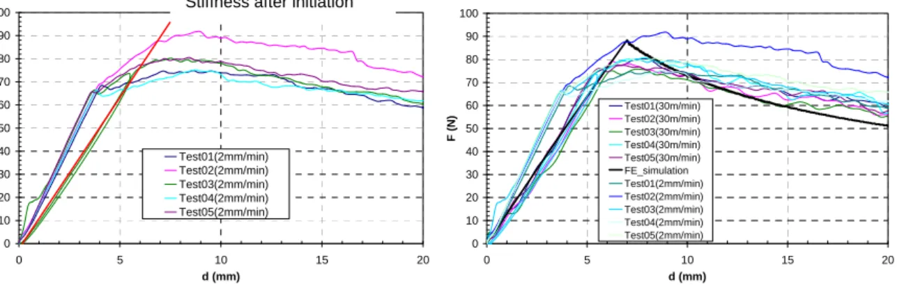
It can be seen in Figure 6 that results of numerical simulation and experimental force displacement curves are very similar. Slightly higher values of peak force and corresponding displacement on numerical curve can be attributed to a bit too stiff mode I numerical model.

0 10 20 30 40 50 60 70 80 90 100 0 5 10 15 20 d (mm) F (N ) Test01(2mm/min) Test02(2mm/min) Test03(2mm/min) Test04(2mm/min) Test05(2mm/min) 0 10 20 30 40 50 60 70 80 90 100 0 5 10 15 20 d (mm) F ( N ) Test01(30m/min)Test02(30m/min) Test03(30m/min) Test04(30m/min) Test05(30m/min) FE_simulation Test01(2mm/min) Test02(2mm/min) Test03(2mm/min) Test04(2mm/min) Test05(2mm/min)

Figure 6: Force displacement curves: quasi-static (LHS) and pseudo-dynamic (RHS)

5 Application to 3D impact delamination

The same methodology has been followed for pure mode II and mixed mode delamination modeling to generate optimal numerical models. Experimental and numerical results are to be published in the forthcoming JNC-16 event [7].

Several impact models were tested to evaluate the ability of this particular model to predict impact induced delamination and mode I participation in a typical case of low velocity impact. In the following paragraphs we present the results of a particular stratification used in aeronautical parts. A coupon specimen of 150 mm × 100 mm × 2.5 mm is simply supported on a metallic support with a rectangular opening of 125 mm × 75 mm. It is impacted by a rigid hemisphere of radius 8 mm at 2.955 m/s (Kinetic energy ~ 10.3 J) using a classical drop weight impact setup.

Finite element model consists of 8 node brick elements with 3 dof per node and 1 integration point for composite plies. One brick element is used per ply. Material properties are shown in Table 2. *CONTACT_ERODING_SINGLE_SURFACE is defined for adjacent plies and zero thickness cohesive elements. Damping is also introduced in the contact algorithm to treat the post failure striking of composites ply parts. The cohesive element related data is same as presented in earlier sections except that the maximum tangential stress in [45/-45] interfaces was chosen to be 40 MPa. Impact model and layering sequence are shown in Figure 7.

Figure 7: ¼ view of 3D numerical mesh model (a) and cohesive zones location and labels (b).

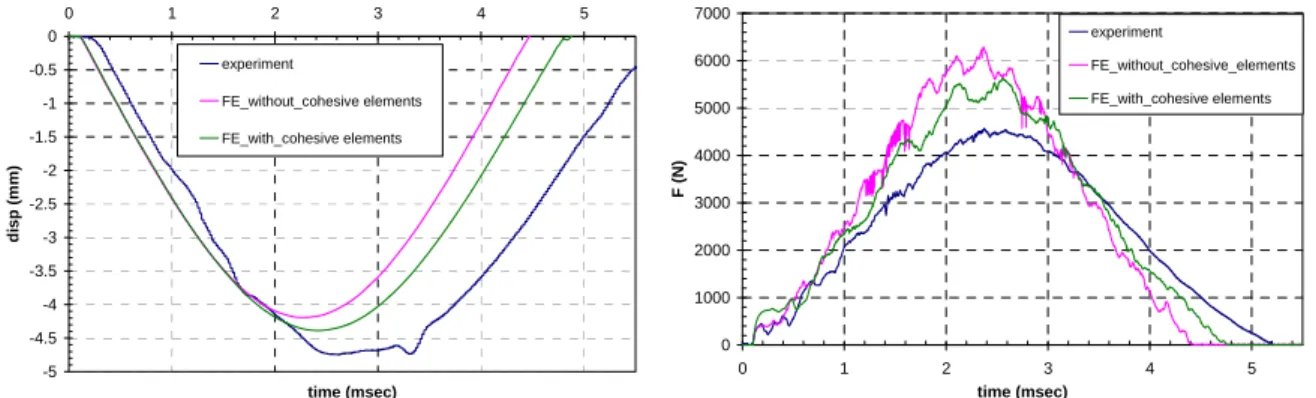
Addition of cohesive elements between the plies in the elastic FE model does not change the global shape of the curves (see Figure 8), neither the loading slopes, but the peak values and the time duration of the contact with the projectile showing the loss of stiffness during the loading phase of the impact. Compared to the experimental force curve, the cohesive model is too stiff. This discrepancy can be attributed to the lack of damage in composite plies. To quantify the inaccuracy part of the cohesive model, delaminated areas are compared with C-scan, and simulations with a ply damage model are carried out, details of which can be found in [8].

Table 2: Orthotropic material parameters

E11 E22 E33 ν12 ν23 ν13 G12 G23 G13

157 GPa 8.5 GPa 8.5 GPa 0.35 0.35 0.53 4.2 GPa 2.7 GPa 4.2 GPa

45 45 -45 -45 0 0 0 0 90 90 Cohesive Coh-1 Coh-2 Coh-3 Coh-4 Coh-5 Coh-6 (a) (b)

-5 -4.5 -4 -3.5 -3 -2.5 -2 -1.5 -1 -0.5 0 0 1 2 3 4 5 time (msec) di sp (mm) experiment FE_without_cohesive elements FE_with_cohesive elements 0 1000 2000 3000 4000 5000 6000 7000 0 1 2 3 4 5 time (msec) F (N ) experiment FE_without_cohesive_elements FE_with_cohesive elements

Figure 8: Comparisons of test and numerical rear face max deflections (LHS), impact forces (RHS) vs. time.

The diameter of the contact area between the projectile and the plate has been measured in the simulations to be around 5 mm (Figure 9). This dimension is a typical length that can be measured in the center the coh-4, coh-5 and coh-6 delamination zones. Cohesive elements have been killed or are almost fully damaged in those zones under the projectile, but the contact is closed between the adjacent layers. Thus, even if the total numerical delaminated area is higher than the experimental measure in the central [0/90] and [90/0] interfaces, they have dimensions similar to the experiment in the external interfaces (around 20 mm length), and the physics of local punch and global flexion is well reproduced. For this observation, we have plotted, in Figure 10, curves of maximum tangential and normal stresses in (i) “correctly” (coh-3) approximated interface, and (ii) “less correctly” (coh-1) approximated interface. Shear stress in both cases shows a global round shape corresponding to the global bending of the plate, and local oscillations during the loading phase of the impact. These oscillations are related to the shock wave that goes back and forth in the thickness direction of plate. In the coh-1 (bottom interface) where the delamination length is inconsistent with the experiment, it is clear that the signal has not been truncated by the maximal tangential stress of 40 MPa, as is the case in the [90/0] coh-3 interface. Delamination could then have been initiated in this interface (coh-3) by a mode II cohesive failure generated by the impact induced wave.

Figure 9: Delamination extension through the thickness at 2.5 ms.

Figure 10: History of maximum tangential stresses (A & B) and normal stress (C) in [-45/45] coh-1 cohesive interface (LHS) and [90/0] coh-3 cohesive interface (RHS).

5 mm Coh-3 delamination

Figure 10 also demonstrates an important fact that the positive normal stresses have lower values as compared to shear stresses. This confirms the observation that delamination initiation and propagation in low velocity impact events are dominated by shear stresses between plies [9].

6 Conclusions

In this paper we have implemented a bilinear cohesive model for delamination simulation. Some of the important numerical parameters that influence the mode I strain energy release rate propagation simulation have been compared. A similar approach can be used to calibrate mode II and mixed mode response. In future cohesive law can be modified to incorporate different initiation and propagation values of GIc.

The application of calibrated model to a more general case of low velocity impact loading has lead us to show that the impact induced delamination is dominated by shear stresses. In future a higher range of impact velocity and incorporation of damage in the composite plies is envisaged.

7 References

[1] Camanho P. P., Dàvila C. G. and De Moura M. F., Numerical simulation of mixed-mode

progressive delamination in composite materials, Journal of Composite Materials, vol 37, 2003, pp 1415-1438.

[2] LS-Dyna Keyword User’s Manual version 971, 2007, pp 535-538.

[3] Pinho S. T., Iannucci L. and Robinson P., Formulation and implementation of decohesion elements in an explicit finite element code, Composites: Part 1, vol 37, 2006, pp 778-789. [4] ISO 15024, Fibre-reinforced plastic composites—Determination mode I interlaminar fracture

toughness, GIc, for unidirectionally reinforced materials, International Standard, © ISO 2001. [5] Maikuma H., Gillespie J. W. Jr., and Wilkins D. J, Mode II interlaminar fracture of the center

notch flexural specimen under impact loading, Journal of composite materials, vol 24, 1990, pp 124-149.

[6] Prombut P., Caractérisation de la propagation de délaminage des stratifiés composites multidirectionnels, PhD thesis, 2007, Université Paul Sabatier, ENSICA, DGM.

[7] Ilyas M., Lachaud F., Espinosa C. and Salaün M., Modélisation de délaminage dynamique des composites unidirectionnels par éléments cohésifs, 16ème Journées Nationale sur les

Composites, 10-12 June 2009, To be presented.

[8] Ilyas M., Lachaud F., Espinosa C. and Salaün M., 17th International Conference on Composite Materials, 27-31 July 2009, To be presented.

[9] Espinosa C., Contribution à l’étude du comportement sous impact localisé basse vitesse de plaques stratifiées à base d’unidirectionnels composites à fibres longues. PhD Thesis, 1991, Université de Metz.