Prime de crédibilité et méthode de l'entropie

(1)

راـتخم يـجاب ةـعماج

ةـباـنع

Annaba

Badji Mokhtar University -

Annaba

Faculté des Sciences

Département de Mathématiques

Laboratoire LaPS

THESE

Présentée en vue de l’obtention du diplôme de

Doctorat 3

ème

cycle en Mathématiques

Option :Statistique Actuarielle

Prime de crédibilité et méthode de l'entropie

Par:

METIRI FAROUK

Sous la direction de

ZEGHDOUDI Halim M.C.A U.B.M. Annaba

Co-directeur

REMITA Mohamed Riad Prof. U.B.M. Annaba

Devant le jury

Année : 2016

PRESIDENT :

BOUTABIA Hacène

Prof.

U.B.M. Annaba

EXAMINATEUR :

HADJI MohamedLakhdar

M.C.A U.B.M. Annaba

(2)

Dedicace

To my parents

To my brother

(3)

Acknowledgement

Firstly, I am extremely thankful to Allah who gave me chance and courage to complete

this work.

I would like to express my sincere gratitude to my advisors Dr. ZeghdoudiHalimfor the

continuous support of my Phd study and related research, for his patience, motivation.

His guidance helped me in all the time of research and writing of this thesis.

Special appreciation to my co-supervisor Prof. Remita Mohamed Riad for his immense

knowledge, his advices despite all the obligations that he had and his love of all

mathematicians .

I would like also to thank the members of my doctoral committee: Prof. Boutabia Hacène,

Dr. Hadji Mohamed Lakhdar and Dr. Brahimi Brahim, who agreed to serve on my

committee on short notice and whose valuable comments will help improve this thesis.

I humbly and gratefully acknowledge the continual and enduring love and emotional

support given by my parents and my brother and sister. I could never acknowledge or

thank my parents enough.

I extend special thanks to Mr. Maroc Azzedine and Mr.Ferdjani Moncef for their

encouragement to finish the thesis.

I would thank all my friends and colleagues and staffs of mathematics department and

university, in particular “Ahmed”.

Special mention must be made here for my intimate friends who supported and

motivated me to continue through the ups and downs towards my goal.

(4)

صخلم

''ردقم وه و لاأ ةيقادصملا ةيرظن يف يساسأ رصنع ةساردب متهن ,ةلاسرلا هذه يف

زيب

''

عيزوت رابتعاب.نيمأتلا طسقل

''

''يلادنيل

سايقملل نييقبسأ نيعيزوت ىلع دامتعلااب و رارضلأا غلابمب صاخ عيزوتك

𝛉

ريغ رخلأا و يتامولعم امهدحأ

''ردقم جارختساب موقن ,يتامولعم

''زيب

ريغ ناتلاد و ةرظانتم ةلاد يه يتلا يعيبرتلا أطخلاةلاد:ةراسخلل لاود ثلاث تحت

: امه و ءاطخلأا باسحب نيتصاخ نيترظانتم

''

linex, entropy

.''

ةلاحلا هذه يف

,

''ردقم

زيب

''

ايطخ لاكش كلمي لا نيمأتلا طسقل

بيرقت ةينقت يه و بيرقتلل ةيددع ةينقت لامعتسلإ انعفدي امم

"

يلادنيل

."

''ردقمل ةيددع ةاكاحم لمعب انمق

''زيب

أطخلا تاعبرم طسوتم ةقيرط ةطساوب

(

MSE

)

أتل

ةيرظنلا جئاتنلا ةحص ديك

لصحملا

.هلاعأ ةروكذملا ةراسخلا لاود فلتخم تحت ردقملا اذه ةنراقم و اهيلع

(5)

Résumé

Dans cette thèse, nous nous proposons, une synthèse sur la théorie de la crédibilité. Plus précisement, nous considérons la distribution de Lindley comme une distribution conditionnelle où nous dérivons l’estimateur de la prime bayésienne sous les fonctions de perte de l’erreur quadratique moyennne, linex et l’entropie avec des distributions a priori informatives et non informatives en utilisant l’approximation de Lindley. Une simulation numérique et une étude comparative sont obtenues.

Mots clés: Distribution de Lindley, Fonction de perte de l’entropie, Méthode des moindres carrées, Prime Bayesienne, Théorie de la Crédibil-ité, .

(9)

In this thesis, we focuse on a popular tool in credibility theory which is the Bayesian premium estimator, considering Lindley distribution as a claim distribu-tion, we derive this estimator under entropy, squared error and linex loss functions with informative and non-informative priors.

The Bayesian premium estimator which is non linear in this case is solved using numerical approximation (Lindley approximation). Simulation study is then per-formed to evaluate this estimator and Mean squared error is computed to compare it under di¤erent loss functions.

Key words: Bayesian premium, Credibility theory, Entropy loss func-tion, Lindley distribufunc-tion, Mean squared error.

(10)

Introduction

L’assurance est une opération par laquelle une personne, l’assureur, s’engage à exécuter une prestation au pro…t d’une autre personne -l’assuré- en cas de réalisation d’un événement aléatoire, le risque (ou sinistre), en contrepartie du paiement d’une somme, cette somme est appelée la prime ou la cotisation.

L’actuaire travaille au sein des compagnies d’assurance. Sa mission: estimer les réserves que la compagnie doit établir pour faire face aux dépenses en fonction des di¤érents contrats signés avec ses clients, calculer les risques et prévoir tous les aléas d’une situation donnée, de manière à faire une tari…cation qui ne laisse aucune place à l’imprévu et qui maximise les béné…ces de la compagnie.

Le calcul de la prime pure est un point fondamental en tari…cation, il a pour but d’évaluer pour chaque assuré le montant attendu des sinistres pour la période d’assurance étudiée. Ce calcul se fait le plus fréquemment par des méthodes statis-tiques comme: les modèles linéaires généralisées (GLM), bonus-malus et experience rating.

La tari…cation basée sur l’expérience (experience rating) en assurance est une technique qui vise à assigner à chaque risque sa prime juste et équitable. Cette prime pour une période dépend exclusivement de la distribution des sinistres de ce risque pour cette période. Cette technique exige un volume d’expérience important. Elle est donc principalement utilisée en assurance automobile et en accidents du travail.

(11)

fois) ou en assurance habitation (fréquence trop faible).

Développée par les écoles suisse et scandinave, la théorie de la crédibilité qui est le pilier d’expérience rating repose sur les principes de l’inférence Bayesienne et représente un ensemble des techniques utilisées par les actuaires pour déterminer la prime d’un assuré/contrat dans un portefeuille hétérogène en utilisant les informations des années précédentes. Elle s’est développée en parallèle de la statistique Bayesienne. Pour un assuré, son risque X est caractérisé par une réalisation notée : Chaque sinistre est vu donc comme une variable aléatoire selon une distribution conditionnelle qui dépend de : En plus, l’espérance des sinistres appelée aussi la prime de risque (individuelle)peut être calculée sur la base de cette distribution conditionnelle.

En pratique, di¤érents modèles ont été proposés pour chercher le meilleur estima-teur de la prime de risque. Le modèle Bayesien quant à lui, consiste à supposer pour une distribution des sinistres à priori ( ) -appelée aussi fonction de structure- qui décrit l’expérience de risque du même paramètre appelée f (x j ).

En combinant la distribution à priori avec la vraisemblancee de f (x j ) ;on peut obtenir la distribution à posteriori f ( j x) qui établit la dépendance de sachant l’historique de l’expérience. La prime Bayesienne PB _{-meilleure prime}

d’expérience-représentant l’espérance des sinistres futurs peut être calculée à partir de f ( j x). Cependant, la prime Bayesienne qui sera chargée à l’assuré est une prime de crédibilité - ayant une forme linéaire- seulement sous une famille de distributions

(12)

et lois à priori conjuguées spéci…ées et aussi sous la fonction de perte de l’erreur quadratique.

PB = z Pexperience+ (1 z) Pcollective (1)

On s’intéresse à une autre fonction de perte qui attribue plus de poids à la surestimation. Dans la théorie de la décision, la fonction de perte de l’entropie (L( ; ^) = ^ q qln ^ 1; q > 0) est une fonction qui donne une importance à la surestimation plus considérablement que la sousestimation.

La forme de cet estimateur dans le cas ou ( ) n’est pas conjuguée est di¢ cile à obtenir à cause des intégrales compliquées.

Pour pallier à ce problème et dériver la prime Bayesienne, on utilise l’approximation de Lindley qui est une méthode numérique d’approximation très utilisée pour résoudre ces formes d’intégrales et qui donne des résultats numériques.

La thèse s’articule autour de trois chapitres, le premier chapitre est consacré aux rappels d’historique et à la formulation mathématique nécessaire de la théorie de la crédibilité. En chapitre 2, on aborde les propriétés de la fonction de perte de l’entropie et on cherche l’expression de l’estimateur de la prime Bayesienne sous cette fonction de perte.

Le troisième chapitre est dédié à l’estimation de la prime Bayesienne dans le cas ou il est impossible d’établir une prime de crédibilité, on utilise une combinaison entre la distribution de Lindley et des lois à priori informatives et non informatives

(13)

tique , linex et entropie). On termine ce chapitre par une simulation numérique et une étude comparative de cet estimateur obtenu sous di¤érentes fonctions de perte. Les conclusions et les perspectives sont données dans le quatrième chapitre.

(14)

Introduction

Experience rating is one of the most important practices in pricing for insurers. In-surance companies set up experience rating systems to determine pricing of premiums for di¤erent groups or individuals based on their past experience. In a competitive market nowadays, insurers want to determine individual premiums as precisely as possible.

Individual policyholders are usually divided into di¤erent groups according to their deemed "risk levels", which are often assessed during the underwriting process based on a variety of relevant factors. A manual rate is then introduced for each group to represent the expected experience arising from the unique risk characteristics of the class.

One implicit assumption embedded in the manual rate is that the underlying risk level is uniformly the same for each member of the class, which is sometimes referred to as "homogeneity" by actuaries. However, as [9] pointed out, there are actually no homogeneous risk classes in insurance. Empirical evidence has suggested that indi-vidual experiences may vary considerably even within the same risk group, because no risk is exactly the same as another. [46] also point out that such heterogeneity may only appear to the insurer through the individual claims records. Therefore, insurance premiums cannot be solely determined by manual rates. Unique individual experiences also need to be taken into account.

(15)

rating, that is, to adjust future premiums based on past experiences. It is used usually in automobile insurance, worker’s compensation premium, loss reserving and IBNR (Incurred But Not Reported claims to the insurer) where credibility theory can be used to estimate the claim size amount.

In this sense, credibility theory is used to determine the expected claims experience of an individual risk when those risks are not homogeneous, given that the individual risk belongs to a heterogeneous collective. The main objective of this theory is to calculate the weight which should be assigned to the individual risk data to determine a fair premium to be charged. Introduction to credibility theory can be found, e.g., in [25], [29], [33], [34], and for recent detailed introductions, one can refer to, for example, [46], which describes its evolutionary history and gives a simple account of its main issues and results, and [9], which gives a comprehensive exposition of the modern credibility theory.

In credibility theory, each risk X of an insured is characterized by a distribution identi…ed by an unknown risk parameter, and due to the heterogeneity over policies in the concerned portfolio, all possible values of are modeled with certain random variable following a probability distribution ( ), which is referred to a structure function in actuarial context and prior distribution in statistical theory. To predict a possible future loss of the risk X or estimate its mean by a quantity (referred to as risk or Bayesian premium PB_{), one observes a sequence of its historical claims}

(16)

and then e¤ectively summarizes information from the observed data (referred to as experience below). Moreover, to the assumed distribution ( ) one can associate a premium (referred to as collective premium below). Consequently, PB _{is represented}

by a credibility form

PB = z Pexperience+ (1 z) Pcollective (2)

However, the credibility premium presented above is restricted by a family of distributions and conjugate prior. Neither the claim distributions which are not members of the exponential family of distributions nor the non-conjugate prior, the predicted mean (Bayesian premium estimator with respect to square error loss) is no longer linear with respect to the data (see [16]) and the credibility formula is no longer true. Whenever the policyholder is undercharged (and insurance company loses its money) or the insured is overcharged (and the insurer is at risk of losing the policy), the square loss assigns similar penalty to over and undercharge. In order to assign more (or less) penalty to overcharged, one has to consider a nonnegative convex function as a loss function rather than square error loss to re‡ect such concerns.

In this case, we may be interested in a loss function which assigned more penalty to overcharges. In decision theory, entropy loss function (given by L( ; ^) = ^

q

qln ^ 1; q > 0) is a popular loss which consider in situation that overestimation is more considerable than underestimation.

It is well known that the Bayesian premium enjoys the advantage of being the esti-mator with the least squared error loss. However, the explicit form of this estiesti-mator in

(17)

di¢ cult to obtain as it involves a number of integrations which are not analytically solvable.

Therefore, one has to use an approximation method for the solutions. Lindley’s approximation technique is one of the methods suitable for solving such problems which approaches the ratio of the integrals as a whole and produces a single numerical result.

In this thesis, our focus will be restricted to determination of Bayesian premium within greatest accuracy credibility theory. One important aspect for this model is the choice of the distribution of losses, which depicts the pattern of the experience of a policyholder conditional upon his risk parameter value. Empirical evidence of-ten suggests that the individual’s claim data can sometimes be volatile and hard to predict.

This thesis is organized as follows. The mathematical formulations underlying the history of credibility theory including Bayesian premium are carefully reviewed in Chapter 1. In Chapter 2, we describe the entropy loss and its properties, we present the expression of the Bayesian premium under this loss when this latter is considered as credibility formula, i.e. under the exponential family. The explicit solution of the Bayesian premium estimator is then obtained.

The Chapter 3 presents our result, we establish the estimation of the Bayesian premium in the case where there is no credibility formula by using a combination

(18)

between lindley distribution and informative and non informative priors.

The Bayesian premium estimator is treated under three loss functions (squared error, linex and entropy) using informative and non informative priors (the extension of je¤rey and the inverted gamma, respectively). Simulation study will be performed and comparisons will be conducted accordingly. Conclusions and future work are presented in Chapter 4.

(19)

Chapter 1 Historical Review Of Credibility

Theory

Credibility theory uses two main approaches, each representing a di¤erent method of incorporating individual experience in the ratemaking process. The …rst and old-est approach is called limited ‡uctuation credibility (also referred to American credibility). According to this approach, an insured’s premium should be based solely on its own experience if the experience is signi…cant and stable enough to be consid-ered credible. The second is called greatest accuracy credibility (also referred to as European credibility).

In the …rst chapter, we present the credibility theory which is a set of quantitative tools used by insurers for performing experience ratings. Two branches of credibility theory, known as limited ‡uctuation credibility theory and greatest accuracy

(20)

credibil-ity theory have also been discussed, we will provide more detailed discussions around mathematical assumptions and formulations of these two approaches.

1.1 Limited ‡uctuation credibility theory

The birth of credibility theory dates back to the beginning of the century with a paper by [43] "How extensive a payroll exposure is necessary to give a dependable pure premium?". In the workers compensation insurance …eld, Mowbray was interested in …nding the minimal number of employees covered by a plan such that the premium of the employer could be considered fully dependable, that is, fully credible.

An individual insured’s premium to be fully credible if it ‡uctuates moderately from one period to another. That is, the credibility criterion is stability. of experience, which usually increases with the volume of the insured’s experience. This volume is expressed as number of claims, number of employees, square foot of factory surface, etc.

With the emergence of theoretic methods, Mowbray’s original problem can be formulated in a slightly more general way as follows.

Let us de…ne the random variables:

Nt = Number of claims generated by the insured during the tth time period

(months, quarters, years, etc.), for t = 1; 2; :::,

Xtj = Size of the jth claim in the tth year, for j = 1; 2; :::; Nt;

(21)

St = Nt

X

j=1

Xtj = Xt1+ Xt2+ ::::::: + XtNt ;

where Xtjs are assumed to be independent, identically distributed (i.i.d) random

variables that are also mutually independent of the Nts. This is the collective model

of risk theory. Most of the situations usually encountered in limited ‡uctuation credibility can be described by an application of this model. It is also well-known (see, for example, [21]) that

8 > > < > > : E [St] = E [Nt] E [Xtj] V ar [St] = E [Nt] V ar [Xtj] + V ar [Nt] E [Xtj]2 :

Let St = (S1+S2+::::::S_T T) denote the insured’s observed average (empirical mean)

claim amount at the end of T periods, T = 1; 2; ::::::

The fundamental problem of limited ‡uctuation credibility is the determination of the parameters of the distribution of St such it stays within 100k percent of its

expected value with probability p; i.e.,

P r[(1 k)E[St] St (1 + k)E[St]] p; (1.1)

holds for given p and k: In a typical limited ‡uctuation credibility situation, the

(22)

1.1.1 Full credibility

When an insured meets the requirements of (1:1), the insured is said to deserve a full credibility of order (k; p) ; i.e., the insured is charged a pure premium based solely on the insured’s own claims experience. If full credibility occurs after T periods, the credibility premium would be ST :

Equation (1:1) thus requires the distribution of ST to be relatively concentrated

around its mean. As ST is a sum of i.i.d random variables, the distribution of ST has

to be approximated.

Assuming the second moment of ST is …nite, one can use the version of the

cen-tral limit theorem applicable to random sums (see [18]; p:258) to approximate the distribution. Thus:

ST E[ST]

q

V AR ST

!n!1N (0; 1);

i.e., a standard normal distribution. (1:1) may then be rewritten

P r[_q kE[St] V AR St S E[St] p V AR[St] kE[St] q V AR St ] 2 [_qkE[St] V AR St ] 1 p; Hence E[St] 2 1 "=2 k 2 V ar [St] T ; (1.2)

Where " = 1 and is the th _{percentile of a standard normal distribution.}

At this point, the essence of the theory of limited ‡uctuation credibility (i.e., equation (1:1)) has been covered.

(23)

premium is granted full credibility and zero credibility below that level. However, an insured with total number of claims just below the full credibility level may pay a signi…cantly di¤erent premium.

The dichotomy between zero and full credibility paved the way for the development of partial credibility.

1.1.2 Partial credibility

The …rst partial credibility formula was developed by Albert Withney In his 1918 paper, Withney refers to "necessity, from the standpoint of equity to the individ-ual risk, of striking a balance between class-experience on the one hand and risk-experience on the other". The objective of credibility theory is the calculation of this balance.

Which principles should govern the calculation of this balance?, According to Withney , the balance depends on four elements: the exposure, the hazard, the collective premium, and the degree of concentration within the class (homogeneity of the entire portfolio).

After some calculations, he obtains the following expression for the individual’s premium P :

P = zX + (1 z) m; (1.3)

(24)

mean. Notice that X and m are combined to produce a weighted average with z and z 1as weights. An expression of the form of (1:3) is called a credibility premium . The quantity z is called the credibility f actor which is given by

z = n

n+k;

Note that k is not an arbitrary constant, rather it is an explicit expression that depends on the various parameters of the model. For the sake of simplicity and to avoid large ‡uctuations between the individual and collective premiums, however, Withney suggests that k may be determined by the actuary’s judgement rather than by its correct mathematical formula.

1.1.3 Uses of limited ‡uctuation credibility

From a theoretical perspective, the range of applications of limited ‡uctuation credibility is fairly limited, though many of these are ignored in practice. the key point to remember when using limited ‡uctuation credibility is that it relies solely on stability criterion, which, generally, is the size of insureds or the number of periods (years quarters, etc) of claims experience. As such, limited ‡uctuation credibility should be used only when stability of the experience is of foremost importance.

The case for partial credibility has been successfully used by American actuaries to restrict premium variation from one time period to another. One can argue that partial credibility takes into account the heterogeneity of the insurer’s block insureds

(25)

among the insureds, however, is only based on their size or the extent of their claims history, this is not necessarily fair.

One must bear in mind that the goal of partial limited ‡uctuation credibility is not to calculate the most precise premium for an insured. The goal is to incorporate into the premium as much individual experience as possible while still keeping the premium su¢ ciently stable. It is important to understand this distinction. When credibility is used to …nd the most precise estimate of an insured’s pure risk premium, one must turn to greatest accuracy credibility methods.

1.2 Greatest accuracy credibility

Greatest accuracy credibility is a more modern, versatile, and complex …eld of credibility theory. It is not a single theory, rather it is an approach to the credibility problem. The main objective is to …nd the best premium to charge an insured, where best is in the sense that the premium estimator is the closest estimator to the true premium.

One important point to keep in mind when moving from limited ‡uctuation to greatest accuracy credibility is that a high credibility factor (i.e., z close to 1) is no longer a goal in itself. Indeed, the credibility factor will henceforth mostly re‡ect the degree of heterogeneity of the portfolio, rather than the degree of stability of an individual’s risk experience. For an homogeneous portfolio, greatest accuracy

(26)

credibility states there is to need to charge a di¤erent premium to the insureds. The credibility factor will accordingly be low, i.e., close to 0. Conversely, the more heterogeneous portfolio, the greater the consideration of the individual experience, hence the higher the credibility factor.

To illustrate this, imagine a portfolio consisting of …ve very large insureds, each having identical means. Given the importance of their size, each group of insureds would all be granted full credibility under the limited ‡uctuation approach. As their means are all equal, however, they form a perfectly homogeneous portfolio. Accord-ingly, their credibility level will be zero under the greatest accuracy approach. Of course, the end result is the same because the collective mean is equal to the individ-ual means, but this shows how di¤erent can be the interpretation of the credibility factor in greatest accuracy credibility.

1.2.1 The mathematical model

Consider an insurance portfolio consisting of I insureds. The ideal situation for ratemaking occurs if this portfolio is relatively homogeneous, i.e., the insureds have similar risks characteristics of insured i that re‡ects the insured’s risk level which is denoted by the risk parameter i for insured i = 1; 2; ::::; I. This risk parameter

incorporates every characteristic of the insured that is not otherwise accounted for in the initial risk classi…cation process.

(27)

we must further assume that each insured’s i is viewed as being drawn at random

from the same cumulative distribution, following [8], ( ) is called the structure or prior f unction.

In a purely Bayesian setting, ( ) represents the insurer’s prior belief about the insured’s risk level. After collection of the insured’s data at the end of the period, the insurer’s initial judgement is revised and the structure function modi…ed accordingly. This interpretation is particularly suited to the case where there is a single insured or when the insurer has little information and must take an educated guess at the initial pure premium for example, when the insurer is entering a new line of business where no data are available.

In the rest of this thesis, we consider the purely Bayesian setting with only one insured (so the subscript i will be dropped). The claim amounts Xt(t = 1; 2; ::::) are

independent and identically distributed, but only given , the risk parameter of the insured. Unconditionally, the Xts are not necessarily independent. The conditional

distribution of X j is denoted by f (x j ).

The determination of a claim amount can be demonstrated with a two-urn model. The …rst urn represents the urn containing the collective with distribution function ( ). From this urn, we select the individual risk, or equivalently its risk level . The parameter then determines the content of the second urn, or equivalently the conditional distribution f (x j ). From this urn, we select the values of the random

(28)

variables X1; X2; :::;

1.2.2 De…nition of various premiums

An underlying tenet of credibility theory is that the estimated premium is the pure or net premium, without any provision for random ‡uctuations, pro…ts, or expenses. Thus two insureds with di¤erent variances but the same mean are charged the same pure premium.

We distinguish here between four types of pure premiums: the individual pre-mium, the collective prepre-mium, the Bayesian prepre-mium, and the credibility premium.

Individual premium (risk premium)

De…nition 1.1 The risk premium, ( ) ; is the correct individual premium to charge an insured if the insured’s risk level, ; is known.

The risk premium is thus the expected value of the insured’s claim amount in one period, given his or her risk level.

(29)

( ) = E [X _{j ] =} Z 1

0

xf (x_{j ) dx:} (1.4)

The individual premium is also referred to as the fair risk premium. Because the risk parameter is unobservable in practice, ( ) can never be exactly known and hence must be estimated from data.

Collective premium

An insurance company insures many kinds of risks. For the purpose of rating risks, these risks are grouped into classes of “similar risks”. In motor insurance, examples of such risk characteristics are cylinder capacity, make of car and power/weight ratio, as well as individual characteristics such as the driver’s age, sex and region. In industrial …re insurance, important characteristics might be the type of construction of the insured building, the kind of business conducted in the building, or the …re extinguishing facilities in the building.

The most important thing for the credibility theory framework is that we do not consider each risk individually but that we rather consider each risk as being embedded in a group of “similar” risks, called the collective.

De…nition 1.2 The collective premium, m, is the pure premium charged when noth-ing is known about the insured’s risk level (durnoth-ing the …rst year, for example). The collective premium is in essence the average value of all possible risk premiums.

(30)

Math-ematically, the collective premium is given by

m = E [X ] = E [E [X _{j ] ] = E [ ( )] :} (1.5)

The fundamental di¤erence between limited ‡uctuation and greatest accuracy credibility is the type of estimator of the risk premium. In limited ‡uctuation credi-bility, the observed claim average X is chosen if the experience is su¢ ciently stable and fully credible, otherwise, the collective mean m is charged. On the other hand, the objective in greatest accuracy credibility is to …nd an estimator as close as possible to the true value of ( )given the available data. There is no unique way to measure closeness. In Bayesian credibility, for example, the most used closeness measure is the mean square error between the estimator and the individual premium.

Bayesian premium (best experience premium)

De…nition 1.3 Suppose the data for n consecutive periods are X1; :::; Xn=X

¯ , then the Bayesian premium PB is given by

PB = min

g(:) E ( ( ) g (X¯)) 2

; (1.6)

where g (:) is some function of the data.

Under the squared error loss, It is no di¢ cult to prove that the solution to this minimization problem is

(31)

PB = E [ ( ) _{j X} ¯] : = Z 1 0 ( ) f ( _{j X} ¯) d : The Bayesian premium can thus be calculated in two steps:

1. First, by calculating the posterior distribution of given the data, f ( j x1; :::; xn) :

Recall that the conditional distribution of X j and the distribution of are assumed to be known in the present model. From Bayes theorem and the conditional indepen-dence of claim amounts, we have

f ( =x1; :::; xn) = f (x1; :::; xn j ) ( ) R f (x1; :::; xn j ) d = n j=1 f (xj j ) ( ) R _n j=1 f (xj j ) d _ ( ) n j=1f (xj j ) : (1.7)

2. Then, by calculating the expected value of ( ) with respect to this distribu-tion: E [ ( )_{j X} ¯] = Z ( ) f ( _{j X} ¯) d : (1.8)

where _ is the proportionality operator, i.e., the right-hand side is equal to the left-hand side up to a multiplicative constant not depending on . Calculation of the expected value is then immediate.

(32)

Here, it should be noted that the experience premium is a random variable (it is a function of the observation vector X

¯), the values of which are known at the time at which the risk is to be rated. The Bayesian premium is thus a “true” premium, the value of which depends on the claim experience.

The last premium to be de…ned before we turn to exact Bayesian credibility is the credibility premium.

Credibility premium

We have seen that the Bayes premium PB = E [ ( )_{j X}

¯] is the best possible estimator in the class of all estimator functions. In general, however, this estimator cannot be expressed in a closed analytical form and can only be calculated by numer-ical procedures. Therefore it does not ful…l the requirement of simplicity. Moreover, to calculate PB_{, one has to specify the conditional distribution as well as the a prior}

distribution, which, in practice, can often neither be inferred from data nor guessed by intuition.

The basic idea underlying credibility is to force the required simplicity of the estimator by restricting the class of allowable estimator functions to those which are linear in the observations X1; :::; Xn. In other words, we look for the best estimator

in the class of all linear estimator f unctions.

“Best” is to be understood in the Bayesian sense and the optimally criterion is again quadratic loss. Credibility estimators are therefore linear Bayesian estimators:

(33)

X1; :::; Xn of an insured, it is a convex combination between the individual experience

weighted average X and the collective premium m; i.e.,

P (X1; :::; Xn) = zX + (1 z) m; (1.9)

where 0 z 1 is the credibility factor and (1 z) is the complement of credi-bility.

It should be noted that the complement of credibility is given to the collective premium, m; and nothing else.

1.2.3 Exact Bayesian credibility

To an actuary who considers himself to be a Bayesian, the Bayesian premium equa-tion PB = E [ ( ) _{j X}

¯] is the best premium (in the least square sense) to charge an insured considering the experience at hand.

The Bayesian premium, however, has some drawbacks when it comes to being used in practice, the actual distributions of X j and must be known.

Moreover, unlike a credibility premium, there is no guarantee that a Bayesian pre-mium will lie between the individual experience average and the collective prepre-mium: This fact can be di¢ cult to explain to a layperson.

Fortunately, there are some combinations of distributions where the Bayesian premium has a nice form. Actually, in these cases, Bayesian premiums are exact credibility premiums.

(34)

We present in below an example of a combination in which, PB is a compromise between X and m.

Example 1.1

suppose X j has a Poisson distribution with parameter , and has a gamma distribution of parameters and , i.e.,

f (x _{j ) =} x_e x! ; x = 0; 1; ::: and ( ) = ( ) 1 e ; > 0; > 0; > 0: The individual premium is

( ) = E [X _{j ] = :} Consequently, the collective premium is

m = E [ ] = : We …nd that the posterior distribution of is:

f ( _{j x}1; :::; xn) _ 1e ni=1

xi_e _;

(35)

+ n;where X

¯ = X1; :::; Xn:The Bayesian premium is thus PB = E ( ( )_{j X} ¯) ; = E ( _{j X} ¯) = ~ ~; = + P ixi n + ; = + nx n + ; = n n + x + 1 n n + ; = zX + (1 z) m;

with z = _n+n : The Bayesian premium is a convex combination between the in-dividual experience average and the collective premium, i.e., a credibility premium with credibility factor z:

[3] was one of the …rst to show that for some combinations of distributions the Bayesian estimator is exactly a (linear) credibility premium. In doing so, Bailey also provided the exact value of the constant k in the credibility factor that [55] choose to determine by judgement. A few years later, [42] extended Bailey’s results.

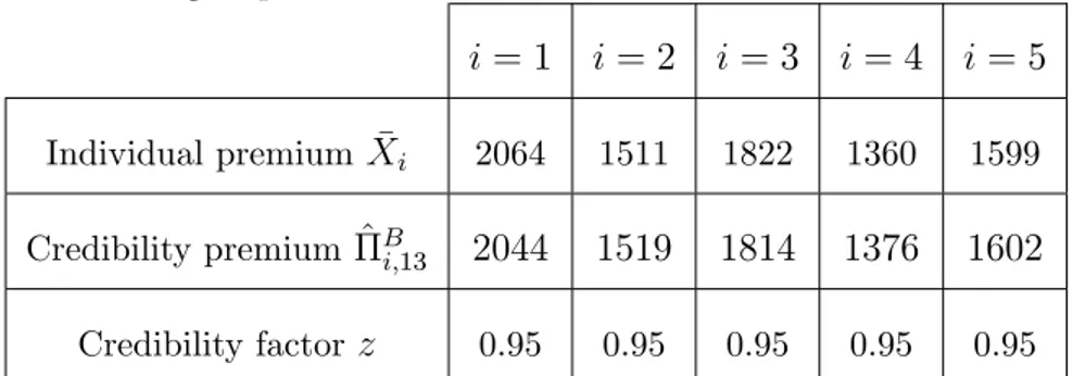
The other combinations of distributions known to yield exact credibility premiums are presented in table (1:1).

(36)

f (x _{j )} Bernoulli( ) Geometric( ) Exponential( ) N( ; 2 1)

( ) Beta( ; ) Beta( ; ) Gamma( ; ) N( ; 2

2)

f ( _{j X}

¯) Beta ~1; ~1 Beta ^2; ^2 Gamma ~3; ~3 N ~; ~

2 2 ( ) 1 1 m ₊ ₁ ₁ PB + P ixi + +n +Pixi +n 1 +Pixi +n 1 n 22x + 21 n 2 2+ 21 z _{n+ +}n _n+n ₁ _n+n ₁ n n+ 2 1 2 2

Table 1.1 - Bayesian credibility models for certain conjugate distributions pairs

~1; ~1 + P jxj; + n P ixj ~2; ~2 ( + n; + P ixj) ~3; ~3 ( + n; + P ixj) ~; ~2₂ 2 2 P jxj+ 21 n 2 2 + 21 ; 21 22 T 2 2 + 21

Table 1.2 - New parameters of the posterior distribution

The table (1:1) contains the distributions which are members of the so-called exponential f amily. [32] uni…ed the results of this table in an elegant way.

Goel in [24] conjectured that only combinations of unidimensional exponential family members with their natural conjugate priors yield linear Bayesian premiums. If Goel is correct, then the only Bayesian premiums that are exact credibility premi-ums are the ones found in the Table 1.1 above.

(37)

We have two practical problems is Bayesian credibility:

The Bayesian premium is a credibility premium in certain cases only,

The premium on subjective assumptions for the distributions of i and Xi j i:

So far we have only considered one particular risk and we have derived the cred-ibility estimator based only on the observations of this particular risk. In practice, however, one usually has observations of a whole portfolio of similar risks numbered i = 1; 2; :::; I:

We denote by X = (X11; :::; XIn)the observation vector of risk with i = 1; 2; :::; I

and t = 1; 2; :::; n: The portfolio is composed of I insureds each characterized by an observable random risk parameter i (risk pro…le). We now assume that for each risk

in the portfolio, i and Xi ful…l the assumptions of the simple credibility model, i.e. i

and Xi are the outcomes of the two-urn model described above, applied independently

to all risks i. We then arrive at the simple Bühlmann model published in the seminal paper “Experience Rating and Credibility” (see [7]).

1.3.1 Model Assumptions

(B1) : The random variables are, conditional on i; independent with the same

(38)

( ) = E [Xij j i] ; 2_{( ) = V ar [X}

ij j i] ;

(B2) :The pairs ( 1 ; X1) ; :::; ( I; Xn)are independent and identically distributed.

Remark 1.2

- By Assumption (B2), an heterogeneous portfolio is modelled. The risk pro…les 1; 2; :::; I are independent random variables drawn from the same urn with

struc-tural distribution ( ). Hence, the risks in the portfolio have di¤erent risk pro…les (heterogeneity of the portfolio). On the other hand, the risks in the portfolio have something in common: a priori they are equal, i.e. a priori they cannot be recognized as being di¤erent.

We now want to …nd the credibility estimator in the simple Bühlmann model. i.e., we want to estimate for each risk i its individual premium ( i). Hence, there is not

just one credibility estimator, but rather we want to …nd the credibility estimators of ( i) for i = 1; 2; :::; I: By de…nition, these credibility estimators ( i) have to

be linear functions of the observations. But here the second question arises: linear in what? Should the credibility estimator of ( i) just be a linear function of the

observations of risk i, or should we allow for linear functions of all observations in the portfolio?. Hence, there are always two items to be speci…ed with credibility esti-mators: the quantity that we want to estimate and the statistics that the credibility estimator should be based on.

(39)

function of all observations in the portfolio, i.e. the Bühlmann credibility estimator

B

i;n+1 of ( i)is by de…nition the best estimator in the class

B i;n+1: B i;n+1 = c i 0+ I X j=1 n X t=1 ci_jtXjt; ci0; c i jt 2 R:

Because of independence between contracts, we know that the credibility premium of contract i is a function of its observations only, we can write it in this form:

B i;n+1= c0+ n X t=1 ctXit:

Taking partial derivatives with respect to c0 and ct, t = 1; :::; n, we have:

c0 = E [ ( i)] n X t=1 ctE [Xit] = (1 nc) m; c1 = ::::::: = cn= c = a an + s2 ; Then, B i;n+1 = ncXi+ (1 nc) m; = zXi+ (1 z) m; (1.10) Where

(40)

z = n n + k = n n + s_a2; Xi = 1 n n X t=1 Xit; k = s 2

a :is called the credibility coe¢ cient,

s2 = E 2( ) ; a = V ar [ ( )] :

Remark 1.3

The structure parameter s2 _{is a global measure of the stability of the portfolio’s}

claim experience. s2 _{is sometimes called the “homogeneity within the insureds”: The}

lower the value of s2; the more stable the portfolio’s claim experience, the larger the credibility factor.

The structure parameter a is a measure of the stability of the various individ-ual risk premiums and is sometimes referred to as the “homogeneity between the insureds”: In other words, a is an indicator of the heterogeneity of the portfolio’s experience. The greater the heterogeneity of a portfolio, the more important is the weight given to individual experience. Hence, as a increases, z increases also.

(41)

Example 1.2 (Poisson-gamma) Taking f (x _{j ) =} x_e x! ; x = 0; 1; ::: and ( ) = ( ) 1 e ; > 0; > 0; > 0:

We know that ( ) = E [X _{j ] =} and 2_{( ) = var [X}

j ] = ; consequently, m = E [ ] = ; s2 = E [ ] = ; a = V ar [ ] = ₂; k = s 2 a = ; z = n n + ; Finally,

(42)

B i;n+1 = n n + Xi+ 1 n n + : Example 1.3 (geometric-beta) Suppose f (x _{j ) = (1} )x; x = 0; 1; ::: and ( ) = ( + ) ( ) ( ) 1₍₁ ₎ 1 ; 0 < < 1; > 0; > 0; ( ) = 1 ; 2_{( ) =} 1 2 ; m = 1; k = s 2 a = 1; z = n n + 1; Then B i;n+1= n n + 1Xi+ 1 n n + 1 1:

(43)

The parametric approach has a limited interest in practice, because its necessity to knowing f (x j ) and ( ) :We assume, as many actuaries do in practical situations, that we know nothing about such probability distributions. These actuaries feel more comfortable in relying exclusively on the data, rather than making subjective judgments about the prior mean and other parameter values. These actuaries estimate the parameters of interest using the available data.

Using the non parametric approach, we replace the pure Bayesian approach by the empirical Bayesian approach.

Estimation of the structure parameters

The structure parameters m; s2_;_{and a are unknown in practice. Hence, they must}

be estimated from the entire portfolio data.

We employ the following estimators for m; s2_;_{and a, respectively:}

^ m = X = 1 I I X i=1 Xi = 1 In I X i=1 n X t=1 Xit; where Xi = 1 n n X t=1 Xit; ^ s2 = 1 I I X i=1 ^ s2_i = 1 I (n 1) I X i=1 n X t=1 Xit Xi 2 ;

(44)

where ^ s2_i = 1 (n 1) n X t=1 Xit Xi 2 ; and ^ a = 1 I 1 I X i=1 Xi X 2 ^s2 n; = 1 I 1 I X i=1 Xi X 2 1 In (n 1) I X i=1 n X t=1 Xit Xi 2 :

It turns out that ^m, ^s2_{, and ^}_a_{are unbiased estimators of m; s}2_;_{and a, respectively.}

The estimators of k and z are then ^k = s^_^_a2 and ^z = n

n+^k; where neither ^k nor ^z is an

unbiased estimator. Finally, the Bühlmann estimate is:

^B

i;n+1 = ^zXi + (1 z) ^^ m; for i = 1; 2; :::; I:

It is possible that â can be negative, an undesirable result since variances must, of course, be nonnegative. In practice, we suppose â0 = max (â; 0) which is a biased estimator. The non parametric approach is illustrated in the following examples.

(45)

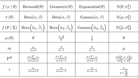
An insurance company has two group workers’ compensation policies. The ag-gregate claim amounts in thousands of dinars for the …rst three policy years are summarized in the table below. Using Bühlmann’s model to estimate the aggregate claim amount during the fourth policy year for each of the two group policies. We don’t make any assumptions about the probability distribution of aggregate claim amounts.

Aggregate claim amounts

Group Policy year

policy 1 2 3

1 5 8 11

2 11 13 12

Table 1.3 - Aggregate Claim Amounts

Solution:

Since there are two group policies and three years of experience data for each, we have I = 2 and n = 3: The observed claim vectors are X1 = (X11; X12; X13) = (5; 8; 11)

and X2 = (X21; X22; X23) = (11; 13; 12)respectively, for the two policies. Since:

X1 = 1 n n X t=1 X1t= 5 + 8 + 11 3 = 8; and

(46)

X2 = 1 n n X t=1 X2t= 11 + 13 + 12 3 = 12;

Then, the estimate of the overall mean, ^m; is

^ m = X = 1 I I X i=1 Xi = 8 + 12 2 = 10; Furthermore, since ^ s2₁ = 1 (n 1) n X t=1 X1j X1 2 = 1 2 (5 8) 2 + (8 8)2+ (11 8)2 = 9; and ^ s2₂ = 1 (n 1) n X t=1 X2j X2 2 = 1 2 (11 12) 2 + (13 12)2+ (12 12)2 = 1;

The estimate of the expected process variance is

^ s2 = 1 I I X i=1 ^ s2_i = 1 2(9 + 1) = 5: The estimate of the variance of the hypothetical means is

^ a = 1 I 1 I X i=1 Xi X 2 s^2 n = 1 1 (8 10) 2 + (12 10)2 5 3 = 19 3 ; Then we have

(47)

^ k = ^ a = 19 3 = 19 = 0:78947;

Next, the estimated credibility factor for each group policy is

^

z = n

n + ^k =

3

3 + 0:78947 = 0:79167;

Finally, the estimated aggregate claim amounts for the fourth year are

^B 1;4 = ^zX1 + (1 z) ^^ m = (0:79167)(8) + (0:20833)(10) = 8:41666; ^B 2;4 = ^zX2 + (1 z) ^^ m = (0:79167)(12) + (0:20833)(10) = 11:58334; respectively. Example 1.5

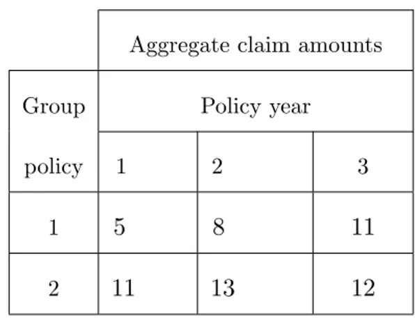
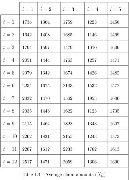
This example is from [25]; which is based on [27]. These informations represent the amount claim in automobile insurance between July 1970 and 1973 in 5 American states. We have I = 5 contracts and n = 12 experience periods. The average claim amounts Xit are presented in the following table.

(48)

i = 1 i = 2 i = 3 i = 4 i = 5 t = 1 1738 1364 1759 1223 1456 t = 2 1642 1408 1685 1146 1499 t = 3 1794 1597 1479 1010 1609 t = 4 2051 1444 1763 1257 1471 t = 5 2079 1342 1674 1426 1482 t = 6 2234 1675 2103 1532 1572 t = 7 2032 1470 1502 1953 1606 t = 8 2035 1448 1622 1123 1735 t = 9 2115 1464 1828 1343 1607 t = 10 2262 1831 2155 1243 1573 t = 11 2267 1612 2233 1762 1613 t = 12 2517 1471 2059 1306 1690

Table 1.4 - Average claim amounts (Xit)

in the Hachmeister portfolio

The estimators of the structure parameters are:

^ m = 1671; ^ s2 = 46040; ^ a = 72310;

(49)

i = 1 i = 2 i = 3 i = 4 i = 5

Individual premiumXi 2064 1511 1822 1360 1599

Credibility premium ^B_i;13 2044 1519 1814 1376 1602

Credibility factor z 0.95 0.95 0.95 0.95 0.95

Table 1.5 - Results with the Bühlmann model

Summary of the non parametric approach

Goal: To determine the compromise estimate of the aggregate claim amount for each of the I policyholders.

Step 1: Determine the number of policyholders, I 2:

Step 2: Determine the number of policy years of experience, n 2

Step 3: Compute the aggregate claim amount, Xit, for each policyholder during

each policy year.

Step 4: Compute the average claim amount, Xi:, over all policy years for each

policyholder.

Step 5: Compute the estimated overall mean, ^m.

Step 6: Compute the estimated expected process variance, ^s2.

Step 7: Compute the estimated variance of the hypothetical means, ^a. Step 8: Calculate ^k = ^s_^_a2:

Step 9: Compute the credibility factor, ^z = n

n+^k:

Step 10: Compute the Bühlmann credibility estimate, ^B

(50)

claim amount for each policyholder. Remark 1.4

Besides Bayesian and Bühlmann models, a number of other credibility models have also been introduced by various researchers like the Bühlmann-Straub model which generalized the Bühlmann model by associating a di¤erent credibility factors for each contract.

Moreover, we …nd models including the random coe¢ cients regression credibility model introduced by [27], the hierarchical credibility model and crossed classi…cation credibility model. For details and formulas see surveys by [7], [9], [10], [26] and [41].

(51)

Chapter 2 Credibility Premium Under

Entropy Loss Function

Under the frequentist paradigm of statistics, every parameter, , is assumed to be a …xed but unknown quantity with an underlying "true value". Statistical inference involves constructing either:

A point estimate of or

A con…dence interval around .

In contrast, under the Bayesian paradigm, every parameter is assumed to be a random variable. Before any data are observed, is assumed to have a particular prior distribution. After the observation of pertinent data, a revised or posterior distribution can be computed for via Bayes theorem.

(52)

A decision problem is generally based on 3 elements: Action (decision) space D:

Set of parameters :

Loss function L( ; ^):

In this chapter, we begin by giving some basic elements about decision theory and loss functions. After, instead of traditional squared error loss function, we de…ne and present the entropy loss function.

2.1 Basic elements

Let ^ 2 D a decision rule.

A loss function L( ; ^) is a measurable function ( _{D) with values in R}+ which

is de…ned as

8( ; ^) : L( ; ^) > 0: 8 ; 9 ~ : L( ; ~) = 0:

In order to obtain a point estimate of from its posterior distribution, it is nec-essary to specify a loss function of , L( ; ^), where we use ^ to denote an estimator of .

We can write L( ; ^): loss, if is the “true” parameter and ^ is the value taken by the estimator when the data is observed.

(53)

of that minimizes the expected value of L( ; ^).

From this, we derive the risk function of the estimator ^

R ; ^ := E hL( ; ^)i= Z

Rn

L( ; ^)dF (x) : (2.1)

The goal then is to …nd an estimator ^ 2 D, for which the risk function R ; ^ is as small as possible. In general, it is not possible to do this simultaneously for all values of i.e. there is no ^ which minimizes R ; ^ uniformly over . In F igure 2:1; we see an example, where depending on the value of , ^1 or ^2 has the smaller

value of the risk function.

(54)

The estimator ^ has two main properties: Admissibility:

^ is admissible if there is no estimator ~ such

R ; ~ R ; ^ ₈ and R 0; ~ R 0; ^ :

If ^ is unique, then ^ is admissible. Minimaxity: ^ is minimax if 8~; sup R ; ^ R ; ~ ; i.e. sup R ; ^ = inf ~ sup R ; ~ : Remark 2.1

In actuarial sciences, when we studying the derivation of credibility premiums, as a statistical decision-making process, some Bayesian premium estimators PB _of

the risk premium ( ) are derived under the symmetric squared error loss function (SELF, henceforth); L( ( ) ; PB) = ( ) PB 2;which is often used also because it does not lead to extensive numerical computation because the Bayesian premium PB _{which minimizes the expected value of the loss function is the mean of the}

pos-terior distribution of , but the SELF considers a same penalty for a policyholder to be under or overcharged and gives no credit to situations in which the policyholder

(55)

ous examples in the literature that suggest the use of loss function associated with estimation or prediction that should assign a more severe penalty for overestimation than underestimation or vice versa (see:[48]; [6]; and [36]). Hence, the use of the symmetric SELF is critical and it is bene…cial to consider some loss functions -like entropy loss- which assigned less or more penalty for being under or overcharged.

2.2 The entropy loss function

In many practical situations, it appears to be more realistic to express the loss in terms of the ratio ^;in this case, [11] proposed a loss function which is called general entropy Loss function (which is also known as Stein loss), it is a useful asymmetric loss when giving credit to under and overestimation which has this form

L( ; ^) = ^ !q

q ln ^ !

1; q_{6= 0;} (2.2)

whose minimum occurs at ^ = ;

q is the loss parameter which re‡ects the departure from symmetry. The loss parameter q allows di¤erent shapes of this loss function. For q > 0, a positive error (overestimation) has a more serious e¤ect than a negative error, and for q < 0, a negative error (underestimation) has a more serious e¤ect than a positive error.

(56)

E hL( ; ^)i= ^

q

E q_jX

¯ q ln ^ + q ln ( ) 1

To achieve the minimum in the above equation, the derivative must be set to zero, namely d d E h L( ; ^)i= q ^ q 1 E q_jX ¯ q ^ = 0; ^q _{= E} q jX ¯ 1 ; ^ = E q jX_¯ 1 q _: _(2.3)

provided that the expectation E q_jX

¯ exists and is …nite.

As we know, the objective in the actuarial science is to …nd the Bayesian estimator of the individual premium ; under the entropy loss, we have

L( ( ) ;PB_ENT) = P B ENT ( ) q q ln P B ENT ( ) 1; q6= 0; Then PB_ENT = E ( ) q_jX ¯ q : (2.4)

In the rest of this work, we assume the original form where q = 1 > 0; which has been used in [14] and [15]: Thus,

(57)

PB_ENT = E ( ) _jX

¯ :

Note that for q = 1, the Bayesian premium under this loss, PB

ENT, coincides with

the Bayesian premium under the SELF.

PB_ENT =PB_SELF:

If we use the exponential family and the conjugate priors, we …nd that the Bayesian premium under the entropy loss function is a credibility premium (compromise be-tween the prior mean and the mean of the current observations) only if q = 1:

Remark 2.2

The usual credibility formula holds whenever

Claim size distribution is a member of the exponential family of distributions,

Prior distribution conjugates with claim size distribution,

Squared error loss has been considered. As long as, one of these conditions is violent, the usual credibility formula no longer holds.

If we change the squared error loss by the entropy loss function (q 6= 1) and taking the copula Poisson-gamma mentioned in example 1.1, we have

PBENT = E ( ) 1 jX_¯ 1 = E 1_jX ¯ 1 = + n +P_ixi 1 1 = + P ixi 1 + n ;

(58)

Thus PB_ENT = n n + X + 1 n + : Bernoulli-Beta: PBENT = E ( ) 1 jX_¯ 1 = E 1_jX ¯ 1 = + + n 1 +P_ixi 1 1 = + P ixi 1 + + n 1; Thus PBENT = n n + + 1X + 1 n + + 1:

we remark that PBENT is not a linear combination of the observation mean and

mean of prior, it is just an a¢ ne function of the observation mean X , then, we have not a credibility formula.

P ayandeh (2010) ;using the mean square error minimization technique, develops a simple and practical approach to the credibility theory. Namely, he approximates the Bayes estimator with respect to a general loss function and general prior distribution by a convex combination of the observation mean and mean of prior, say, approximate credibility formula.

It is well known that Bayes estimator re‡ects properties of loss function and prior distribution (see Marchand and Payandeh, 2009). Therefore, it makes sense to consider a Bayes estimator, under an appropriate loss and prior distribution, as

(59)

parameter.

The following lemma considers a Bayes estimator as an appropriate estimator for parameter. Then, using the mean square error technique develops a new approach to approximate the Bayes estimator by the credibility formula.

Lemme 2.1 (P ayandeh 2010) : Suppose X1; X2; :::; Xngiven risk parameter are

iden-tical and independently distributed with ( ) = E [X _{j ] for i = 1; 2; :::; n: Moreover,} suppose that the risk parameter has a prior distribution with mean m , i.e., m = E [ ], and PB is a Bayes estimator with respect to loss function L and prior distribution .

Then, in the class of credibility premiums

P = Pz :where Pz = zX + (1 z) m; and z 2 [0; 1]

an estimator Popt; with

zopt =

E X m PB m

E X m 2 ; (2.5)

minimizes the mean squared error between PB _{and P} z; i.e.,

Popt = arg min E PB Pz 2

(60)

Proof. Mean square distance between two estimators PB and Pz can be readily

observed as

M SE (z) = E PB Pz 2

= E PB zX (1 z) m 2:

Taking derivative with respect to z @M SE (z)

@z = 2E X m

2

2zE X m PB m = 0;

Along with the fact that second derivative of M SE (z) with respect to z,

M SE00(z) = 2E X m 2; is nonnegative lead to the desire result.

Two-folded expectations in nominator and denominator of zopt given, the above

can be simpli…ed as E X m PB m = E cov X;PB _j + cov E X _j ; E PB _j + (m0 m) mP B m : where m0 = E [E [Xi j ]] ; mPB = E E PB _j for i = 1; 2; :::; n:

(61)

approximate credibility premium, given by Popt, coincides with the exact one.

Proof. If the exact credibility premium holds, the Bayes estimator PB can be written as PB _{= zX + (1} _{z) m. From this fact, one can observe that}

zopt = E X m PB m E X m 2 = E X m zX + (1 z) m m E X m 2 = E X m zX zm E X m 2 = zE X m X m E X m 2 = z:

(62)

Chapter 3 Bayesian Premium Estimators

under Squared Error, Entropy and

Linex Loss Functions: with

Informative and Non Informative

Priors

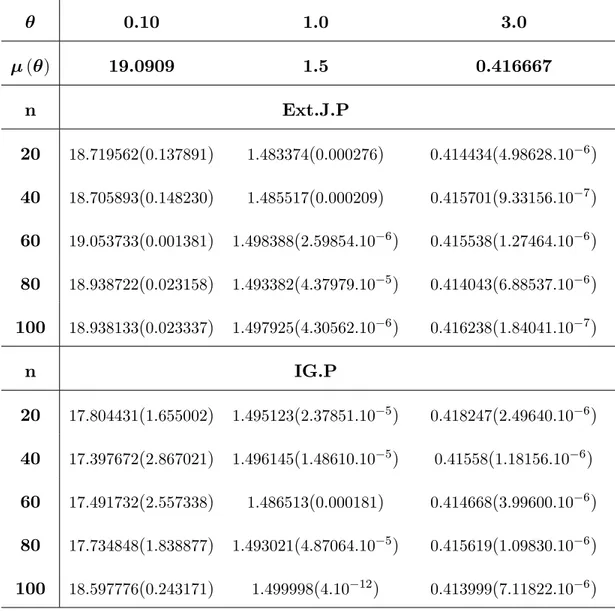
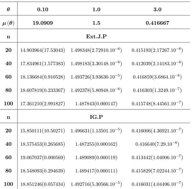
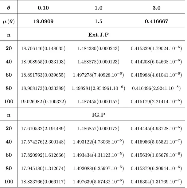
In this chapter, considering the Lindley distribution as conditional distribution of X j ; we focus on estimation of the Bayesian premium under three loss func-tions (squared error which is symmetric, linex and entropy which are asymmetrics), using non-informative and informative priors (the extension of Je¤reys and Inverted

(63)

ical approximation for computing the Bayesian premium.

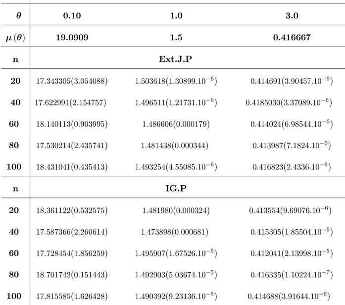
A comparison was made through a Monte Carlo simulation study on the perfor-mance of these estimators according to the mean square error (MSE). Results are summarized in tables and followed by concluding remarks.

3.1 Around Lindley distribution

In Bayesian analysis, the unknown parameter is regarded as being the value of a random variable from a given probability distribution, with the knowledge of some information about the value of parameter prior to observing the data x1; x2:::; xn.

The Lindley distribution is one of the most popular distributions of waiting time and reliability theory. It was originally developed by [39] and some classical statistics properties are investigated by [23]. [37] considered Lindley distribution for reliability estimation using maximum likelihood and Bayesian approach. [51] introduced a dis-crete version of Lindley distribution known as disdis-crete Poisson-Lindley distribution.

The distribution of zero-truncated Poisson-Lindley was introduced by [23] and [56] introduced the Negative Binomial distribution as an alternative to zero-truncated Poisson-Lindley distribution. [22] introduced a two parameter weighted Lindley dis-tribution and pointed that Lindley disdis-tribution is particularly useful in modeling biological data from mortality studies. In addition, [57] introduced a new distrib-ution, named gamma Lindley distribdistrib-ution, based on mixtures of gamma (2; ) and

(64)

one-parameter Lindley distributions which is useful in modeling lifedata. Recently, a study of the e¤ect of some loss functions on Bayes Estimate and posterior risk for the Lindley distribution are made by [50]:

Let x1; x2; :::; xn be independent and identically distributed from Lindley

distrib-ution with an unknown parameter . The probability density function is given by: 8 > > < > > : f (x; ) = 2_(1+x)e x 1+ ; x; > 0 0; otherwise. (3.1)

It can be written as a mixture of gamma distribution (2; ) with exponential distribution ( ), where p1 = ₊₁ and p2 = 1 p1:

The corresponding cumulative distribution function (c.d.f.) is:

F (x) = 1 + 1 + x

+ 1 e

x_; _{x > 0;} _{> 0:}

Many authors showed that (3:1) provides a better model for waiting times and survival times data than the exponential distribution.

However, due to the popularity of the exponential distribution, the Lindley dis-tribution has been overlooked in the actuarial literature and in many applied areas.

The expectation and the variance of Lindley distribution are

( ) = E [X _{j ] =} + 2 ( + 1); 2_{( )} _{= var [X} j ] = 2_{+ 4 + 2} 2 ( + 1)2 :

(65)

ley distribution is: L (x; ) = 2 1 + n n i=1(1 + xi) e Pn i=1xi_{; x;} _{> 0} _(3.2)

The logarithm of likelihood function is

ln L (x; ) = n ln 2 ln (1 + ) + n X i=1 ln (1 + xi) n X i=1 xi: Maximizing for d ln L (x; ) d = 0: We get x 2+ (x 1) 2 = 0; > 0:

Solving for we have

^ = 1 x +

q

(x 1)2+ 8x

2x :

It can be written under the form p(x)e_{q( )} x with p (x) = 1 + x;

(66)

q ( ) =

2

1 + ;

which means that it’s a member of the exponential family,

It is well known that, for Bayesian premium estimators, the performance depends on the form of the prior distribution and the loss function assumed.

3.2 Derivation of Bayesian premiums

To obtain Bayesian premium estimators, we assume that is a real valued random variable with probability density function ( ). Recall that the conditional distrib-ution of X j is the Lindley distribution and the distribution of is assumed to be known in the present section.

f ( _{j X}

¯) is the posterior distribution of given the data. In this section we consider the estimation of the Bayesian premium PB _{based on the above mentioned}

priors and loss functions.

3.2.1 Bayesian premium estimators under squared error loss

function

The squared error loss function was proposed by [38] and [10] to develop least squares theory. It is de…ned as

(67)

L(^; ) = ^ ;

To obtain Bayesian premium estimators, we write

L(PBSELF; ( )) = P B

SELF ( )

2

;

The Bayesian premium PBSELF is the estimator of the individual premium ( ), it

is to be chosen such that the posterior expectation of the squared error loss function

E L(PBSELF; ( )) = Z 1 0 L(PBSELF; ( ))f ( j X ¯) d = Z 1 0 PB_SELF ( ) f ( _{j X} ¯) d ; is minimum. Here PB_SELF = E [ ( ) _{j X} ¯] : (3.3) = Z 1 0 ( ) f ( _{j X} ¯) d ; ((3.4)) where ( ) = E [X _{j ] =} + 2 ( + 1); is the individual premium.

(68)

Posterior distribution using the extension of Je¤reys prior

Bayesian approach makes use of ones prior knowledge about the parameters as well as the available data. When ones prior knowledge about the parameter is not available or very little, it is possible to make use of the noninformative prior in Bayesian analysis.

Since we have no knowledge on the parameters, we seek to use the extension of Je¤reys’prior information, where Je¤reys’prior is the square root of the determinant of the Fisher information.

We …nd Je¤rey prior by taking ( ) =pI ( ); where

I ( ) = E @ 2_{ln f (x; )} @ 2 = 2_{+ 4 + 2} 2 (1 + )2 ; is the Fisher information.

The extension of Je¤reys distribution is assumed as non-informative prior for the parameter : It was proposed by [2] and [30], it is given as:

( ) = [I ( )]c = k 2 + 4 + 2 2_{(1 + )}2 c ; ; c > 0; k is a constant. (3.5)

Combining (3:5) with the likelihood function of the Lindley distribution, the pos-terior distribution of parameter given the data (X1; X2:::; Xn) is derived as follows:

(69)

f ( _{j X} ¯) = n i=1L (xi ; ) ( ) R1 0 n i=1L (xi ; ) ( ) d = 2(n c) (1+ )n+2c 2_{+ 4 + 2} c_e Pn i=1xi R1 0 2(n c) (1+ )n+2c 2_{+ 4 + 2} c_e Pn i=1xid ; > 0

According to the squared error loss function, the corresponding Bayesian premium estimator is derived by substituting the posterior distribution (3:5) in (3:3), as follows:

PB_SELF = Z 1 0 ( ) f ( _{j X} ¯) d = R₁ 0 2(n c) 1 (1+ )n+2c+1 2_{+ 4 + 2} c_{( + 2) e} Pn i=1xi_d R₁ 0 2(n c) (1+ )n+2c 2_{+ 4 + 2} c_e Pn i=1xid ; > 0 (3.6)

We know that only combinations of unidimensional exponential family members

with their natural conjugate priors yield linear Bayesian premiums (exact credibility formula) which are mentioned in the Table (1:1).

It may be noted here that the posterior distribution f ( j X_¯) takes a ratio form that it give not a credibility formula and involves an integration in the denominator and cannot be reduced to a closed form. Hence, the evaluation of the posterior expec-tation for obtaining the Bayesian premium of will be tedious. Among the various methods suggested to approximate the ratio of integrals of the above form, perhaps the simplest one is Lindley’s (1980) approximation method, which approaches the ratio of the integrals as a whole and produces a single numerical result. Thus, we propose the use of Lindley’s (1980) approximation for obtaining the Bayesian premium. Many

(70)

authors have used this approximation for obtaining the Bayes estimators for some distributions, see among others, [28] and [31].

If n is su¢ ciently large, according to Lindley (1980), any ratio of the integral of the form I (x) = E [h ( )] = R h ( ) exp [L ( ; x) + g ( )] d R exp [L ( ; x) + g ( )] d ; > 0 (3.7)

where h ( ) = function of only, L ( ; x) = log of likelihood, g ( )= log of prior of . Thus,

I (x) = h ^ + 0:5h ^h + 2^h ^p ^ i+ 0:5h ^h ^ L^ ^ i (3.8) where ^ = mle of = (x 1) + q (x 1)2+ 8x 2x ; x > 0: ^ h = @h ^ @^ ; ^ h = @2h ^ @^2 ;

(71)

^ p = @^ ; (3.9) ^ L = @2L ^ @^2 ; ^ = 1 ^ L ; ^ L = @3_{L ^} @^3 :

After substituting the value of f ( j X_¯), it may be written as:

PBSELF = E [ ( ) j X ¯] = R ( ) exp [L ( ; x) + g ( )] d R exp [L ( ; x) + g ( )] d ; > 0 (3.10) Where h ( ) = ( ) = + 2 ( + 1); L ( ; x) = 2n ln n ln (1 + ) n X i=1 xi+ n X i=1 ln (1 + xi) ; g ( ) = c ln 2+ 4 + 2 2 ln 2+ ;

(72)

^ h = 2 + 4 + 2 2₊ 2 ; ^ h = 2 4_{+ 14} 3_{+ 24} 2_{+ 16 + 4} 3 ( + 1)4 ; ^ p = 2c ₂ + 2 + 4 + 2 2 + 1 2₊ ; ^ L = 2n₂ + n (1 + )2; ^ = 2_{(1 + )}2 2n (1 + )2 n 2; ^ L = 4n₃ 2n (1 + )3; Then, we get PBSELF = E [ ( )j X ¯] = ^ + 2 ^ ^ + 1 + 2 6 6 6 4 2 6 6 6 4 ^4 +7^3+12^2+8^+2 ^3 (^+1)4 + 2c _^2^+2 +4^+2 2^+1 ^2_+^ ^2_+4^+2 ^2 +^ 2 ! 3 7 7 7 5 ^2 _{1 + ^} 2 2n 1 + ^ 2 n^2 3 7 7 7 5+ 2 6 4 2 6 4 ^2 _{1 + ^} 2 2n 1 + ^ 2 n^2 3 7 5 22 6 4 n 1 + ^ 3 2n ^3 3 7 5 2 6 4 ^2_{+ 4^ + 2} ^2_{+ ^} 2 3 7 5 3 7 5 : (3.11)