Features selection approaches for an objective control of cosmetic quality of coated surfaces

This is an author-deposited version published in: https://sam.ensam.eu Handle ID: .http://hdl.handle.net/10985/18718

To cite this version :

S BESSONNET, M EL MANSORI, S MEZGHANI, Nicolas CONIGLIO, R PEE, S PINAULT Features selection approaches for an objective control of cosmetic quality of coated surfaces -Surface Topography: Metrology and Properties - Vol. 8, n°2, p.024007 - 2020

Any correspondence concerning this service should be sent to the repository Administrator : archiveouverte@ensam.eu

Features selection approaches for an objective

control of cosmetic quality of coated surfaces

S. Bessonnet

, M. El Mansori

, S. Mezghani

, N. Coniglio

, R. Pee

, S. Pinault

1 Arts et Métiers ParisTech, MSMP Laboratory, Rue Saint Dominique, BP 508, 51006 Châlons-en-Champagne, France 2 Arts et Métiers ParisTech, MSMP Laboratory, Cours des Arts et Métiers, 13617 Aix-en-Provence, France

3 Texas A&M Engineering Experi ment Station, College Station, TX 77843, USA 4 ESSILOR International, 63 Boulevard Oudry, 94000 Créteil, France

* _{Corresponding author: Tel: +33 (0)6 25 05 62 95 Email: stephanebessonnet@gmail.com}

Received Date Line (to be inserted by Production) (8 pt)

Abstract

The cosmetic aspect is one of the main functions of industrial surfaces in numerous applications. Even the smallest surface defects may have a critical effect on the cosmetic tolerability of such industrial surfaces. Thus, surfaces are generally coated at the last manufacturing process stage to cover existing defects and to certify their cosmetic quality. The surface quality is however constantly controlled after coating that induces an increase of lead-time increase and production costs. This is due to a various flaw patterns and a lack of uncoated surfaces specifications. Hence, the identification of relevant surface morphological parameters underlies an objective and automatic cosmetic control performance. In fact, this relevant parameter selection allows tracking surface flaws during the coating finishing operation.

This paper presents a comprehensive overview of various feature selection tools for data analysis (Neighbourhood Component Analysis (NCA), ReliefF, Sequential wrapper method, Decision tree) to extract relevant information out of physical data. A design of experiment based on scratches test on amorphous polymers to generate typical controlled defects has been performed. Then, several cosmetic defects characteristics were extracted from experimental measurements. Feature selection approaches were applied and compared to determine the most relevant parameters. The advantages and limitations of each method for data analysis have been highlighted in the case of real engineering surface quality control.

Keywords: feature selection, cosmetic quality, surface defects, coating.

1. Introduction

Glassy polymers are usually used in optical applications like lenses (safety, or ophthalmic lenses), displays (aquarium displays) or protection (motorcycle visors) for their specific property to be transparent. The integrity of the surface is linked to the cosmetic appearance of the surface [1-4]. The cosmetic appearance is often difficult to quantify, and it is linked to human perception. The judgment and the expertise of a specialized operator is required for lens control. An operator checks for numerous types of surface defects like scratches, pits, and burnings after each key step of the finishing process. The focus for this study is scratches. A scratch is a defect which scatters light. It can become visible to the customer and decrease the quality of the surface [5].

A complex process called surfacing [3] is used to obtain the final surface of the polymer. Then, the surface is coated by a harder and transparent coating to make the polymer less sensitive to environment aggressions and to protect the surface integrity during the product life. Additionally, the coating has an optical filtration effect on the surface which allows some defects that are visible before the coating step to disappear after being coated. It is common practice today to conduct a first cosmetic control after the surfacing stage and a second after the coating stage to check the integrity of the polymer surface. If the surface is not in compliance with a certain standard, it will be rejected. However, there are many inaccuracies in the control. Some surfaces are rejected after the surfacing stage even though they are suitable for coating and some others that are validated after the surfacing stage are rejected after the coating.

To reduce the cost and to increase productivity, a laboratory method based on scratch experiments and statistical learning modelling is proposed. It streamlines the cosmetic control by classifying the surface only once after the surfacing stage. The classification inputs used for the models are limited to morphological surface parameters. This is because scratch can also occur due to a deviation during the surfacing process, a wrong manipulation of the equipment, or others erratic sources. The morphological surface parameters are independent of these sources of error. Consequently, this allows the operator to control for the surface and not the source of defects. A second aim of this classification is to evaluate the contribution of the inputs towards scratch formation. These inputs are the outputs of the previous process. The surface parameters that are analysed are surfacing targets for the polymer’s cosmetic appearance.

2. Experimental procedure and the dataset realisation

The objective of the experimental part of the study is to reproduce typical scratches observed during the cosmetic control of the lenses. MR7, a high optical index polymer, has been chosen for this study. It is produced by the Mitsui Company and is usually used for complex optical products. Table 1 shows the material properties of MR7 polymer.

Table 1 MR7 material properties

Property Value

Thermophysical Glass transition temperature (Tg) 93°C

Mechanical

Elastic modulus 4.4 GPa

Impact resistance 180 J/m²

Hardness 196 MPa

Physical Specific gravity 1.36 g/cm3

Optical Refractive index 1.665

Abbe number 30.3

MR7 samples were cut with machining processes comprising milling and diamond turning to obtain cylindrical shapes 1.5mm in height and 25mm in radius. The surfaces of the samples were finished by a free abrasive polishing process. The free abrasive particles scratch the surface stochastically, creating a smooth and transparent surface. The scratch dimensions depend on the particles’ shape and size. The surfaces were controlled to ensure that there were no visible scratches on the surface from the polishing (Fig 1) or the cleaning of the sample.

Next, the scratches were performed and characterised, following which the samples were coated by a dip-coating process. The workpiece is immersed in a varnish tank and drawn at constant speed. The dip-coating adheres by capillarity to the surface. The thickness of the coating is depending of the viscosity and the drawn speed. In this investigation, those parameters are maintained constant during the test. The coating thickness is about 3 µm on each face of the sample.

The surfaces were scratched with a Morphoscan Michalex (Fig 2.a) device at 20°C room temperature and 24% relative humidity. A load cell in the equipment controls an indenter to penetrate the surface and create the scratch. The sample is placed on top of an XY table which moves to propagate the scratch. The tests were performed with a controlled force and a constant velocity (100µm/min). Five indenters were used: a Berkovitch indenter and four spherical indenters with 2, 5, 10 and 20µm radius. The sizes of the four spherical indenters were chosen to fall within the free abrasive particle size distribution so as to simulate polishing scratches. The aim is to get several morphologies of the scratch with the different indenters.

Figure 1: Interferometer measurement of the polished surface of an MR7 sample

A total of 7 scratches were made on each surface: six with a constant load across the length of the scratch and one with an increasing load following a step function. The step function ranges from the minimum to the maximum load used on the constant load scratches. 11 load steps increasing linearly from the minimum to maximum were made. The objective is to test whether the behaviour of the coating is the same between a constant load and an increasing load.

Each sample is tested with one of the six indenters and one of three ranges of loads: 0-50 mN, 60-260mN and 300-500mN. The loads are shown in Table 2. The loads are described on the Table 2, three range of force were tested on each indenter: 0-50 mN, 60-260mN and 300-500mN. We note RH the scratches on the top of surface presented in figure 2.b, and we numerated them from 1 to 3, from the left to the right. The RB scratches are those made on the bottom of the surface. The RL scratch is the increasing scratch on the extreme left of the surface, the forces used during the scratch are detailed on the Table 2.

Figure 2: a) Morphoscan machine, b) Position of the scratches on the sample

Table 2: Summary of forces used for the scratches

During scratching, some of the polymer material in the furrow is pushed out to form ridges at the side. Those ridges could perturbate the coating flow. Hence, the scratches are spaced 8 mm apart to avoid any interactions between neighbouring scratches (Fig 2.b).

Characterisation of the scratch topography was done after allowing some time for material springback to occur [6]. The scratch topography was measured with a white-light Veeco interferometer (WYKO3300NT), which is an optical surface profiler. An area of length 1 mm and width between 56µm and 150µm was selected. The width was adapted to fit the scratch. The sampling is 192 nm. Then, 10 cross-sections were extracted from the selected areas, and seven parameters were computed (Fig 3.a):

 Depth: the vertical distance between the lowest point of the scratch and the mean line,  Exterior width: the horizontal distance between both ridges’ furthest point,

 Interior width: the horizontal distance between the highest point of both ridges,

b)

a)

 Ridge width: the horizontal distance between the points where the ridge goes above the mean plane. The larger ridge width of the two is taken,

 Ridge height: the vertical distance between the mean plane and the highest point of both ridges,  Slope: the absolute value of the angle between the vertical and the slope of the scratch on the mean

plane line. The average of the two slopes is taken,

 Area: the empty space between the mean plane line and the bottom of the scratch furrow.

Figure 3: a) extracted parameters from the scratch cross-section from b),

b) scratch measurement with a white light interferometer

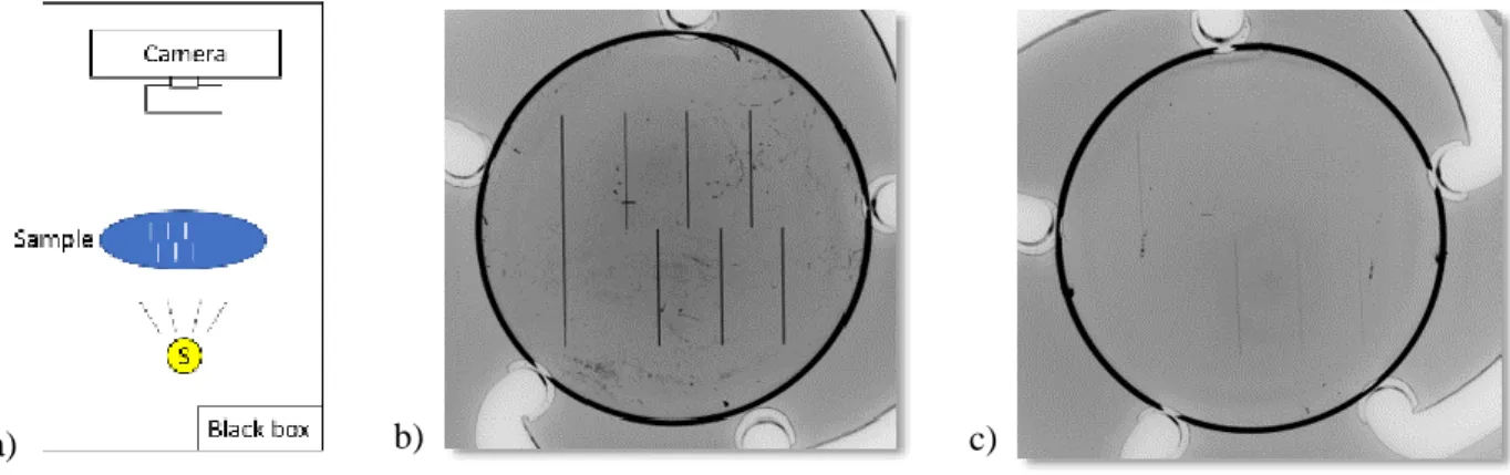
The scratches are classified into two classes: invisible or visible indexed with a Boolean criterion 1 and 0 respectively. The decision to classify a scratch as visible or invisible was made with a high-resolution picture taken in a controlled environment. The setup contains a black box used to remove parasitic light and a light source placed under the sample. The sample is laid on a support and a camera that is aligned above takes a photo (Fig. 4.a).

Figure 4: a) schema of the black box to take picture, b) picture of the sample before the coating (60-260 mN, 10µm spherical indenter) c) picture of the sample (b) after the coating (All RB scratches are visible, the RH3 is visible, then the RH2 and the RH1 are not visible)

b)

a)

First, the relationships to scratch visibility were explored relative to individual scratch parameters, but the visibility does not seem to be defined by a single parameter. Some parameters like the slope and the area are randomly distributed on either side, while others like the depth and the width parameters are not definitive. For instance, for the interior width (see Fig 4), if it is larger than 1µm, a scratch has a high chance to be visible. If it is larger than 2µm, a scratch will be completely visible. The interior width between 1 and 2 µm defines what we call the undetermined area for the classification. For a cosmetic control, the error will focus inside the undetermined area. A single parameter is not enough to definitively classify a scratch but using all of them will be too many parameters to follow for a streamlined control. The feature selection method is used in the following section to find an optimal subset to predict the classification of the scratch and to reduce or to eliminate the undetermined area.

Figure 5: Boolean decision versus the Depth, the Interior width, the Slope, and the Area. 3. The feature selection method

The feature selection approaches are divided into three categories: the filter, the wrapper and the embedded method. The performance of the method is mainly dependant of features and outputs because the algorithms are adapted of different kind of inputs and output relationships. Hence, several methods are considered for an overview of the classification.

3.1 The filter method:

In the feature selection approach, the filter method defines an optimal subset according to an independent measure like a distance (Euclidean or Manhattan distance). The filter method does not use any learning algorithm. Hence, they are often easier to code. However, filter methods omit the interaction between the features because the methods measure only the relevancy of the individual feature and not combinations of features. [7-16]

The NCA [15] algorithm is based on the neighbourhood component analysis (NCA). The goal is to define a

classification function f : ℝ𝑝_{→ {0,1}. The NCA uses a random reference element Xref from the data set. It evaluates}

the probability for an element Xi to be inside the class of Xref. This probability is estimated with the distance between the elements. It assumes that:

𝑃(𝑋𝑖∈ 𝑐𝑙𝑎𝑠𝑠(𝑋)) ∝ 𝑘 ∗ 𝑑𝑤(𝑋𝑟𝑒𝑓, 𝑋𝑖) (1)

The distance between Xi and Xj is computed as:

𝑑𝑤(𝑋𝑖, 𝑋𝑗) = ∑ 𝑤𝑝𝑟2|𝑋𝑖𝑟− 𝑋𝑗𝑟|

𝑝

𝑟=1

(2)

where 𝑤𝑝𝑟 is the weight of the variable in the classification. In our case, the function learns the feature weights by

a diagonal adaptation of neighbourhood component analysis (NCA) with regularization [15-16]. The method gives an optimal subset and the contribution of each parameter.

ReliefF:

The Relief-F method is an extension of the Relief algorithm developed by Kira and Rendell [13]. The ReliefF method is based on iterative adaptation of the given weight of the feature. A random Xi is taken and the algorithm searches the k nearest neighbours from the same group and the k nearest neighbours from each of the different groups. The k first is named the nearest hits Hj and the second group is called nearest misses Mj. The contribution of each group of the misses is weighted with the priority of group P(G). The weights of the feature F are updated with [9, 12, 17]: 𝑊[𝐹] = 𝑊[𝐹] − ∑𝑑𝑖𝑓𝑓(𝐹, 𝑋𝑖, 𝐻𝑗) (𝑚 ∙ 𝑘) 𝑘 𝑗=1 + ∑ [ 𝑃(𝐺) 1 − 𝑃(𝐺𝑟𝑜𝑢𝑝(𝑋𝑖)) ∗ ∑𝑑𝑖𝑓𝑓 (𝐹, 𝑋𝑖, 𝑀𝑗(𝐺)) (𝑚 ∙ 𝑘) ] 𝑘 𝑗=1 𝐺≠𝐺𝑟𝑜𝑢𝑝(𝑋_𝑖) (3) Where the function diff(F, X1, X2) is:

𝑑𝑖𝑓𝑓(𝐹, 𝑋1, 𝑋2) = {0 ; 𝑣𝑎𝑙𝑢𝑒(𝐹; 𝑋1

) = 𝑣𝑎𝑙𝑢𝑒(𝐹, 𝑋2)

1 ; 𝑜𝑡ℎ𝑒𝑟𝑤𝑖𝑠𝑒 (4)

ReliefF can also classify with missing data and produce multiples outputs whereas the Relief cannot. ReliefF does not return any subset but only the contribution of each parameter. Hence, the choice of the subset is often made using a few handpicked parameters or a threshold which defines the most relevant parameters.

3.2 The wrapper method:

The wrapper methods are usually more relevant than the filter methods because they use a learning algorithm. [7] The method evaluates each subset and not only the individuals feature to define the relevancy of the subset. The wrapper approaches select an optimal subset of features for the modelling. However, they are slower than the other methods because they check each subset successively, hence they are time-consuming and computing-intensive for a large number of features. The hybrid method (filter following by a wrapper method) is proposed to retain the classification performance with the wrapper method and evaluation of the most relevant inputs with the filter method. [9,12,17]

Forward sequential selection method (FSS):

FSS [14] is one of the most natural methods for finding the best feature subset. The algorithm starts with an empty subset and adds one feature into the subset. Then, all the combinations with two features are tested and if a combination is better than the single subset, the new feature is added. The algorithm continues with three features and so on. When the subset cannot be improved further, the algorithm stops and returns the subset as the optimal subset. A function which outputs a value for each subset is used to compare subsets.

The algorithm can be performed in the forward and backward directions. The forward algorithm starts with an empty subset and adds new features. On the contrary, the backward algorithm starts with the full set and removes features from the subset.

The algorithm returns an optimal subset without indication of the feature contributions. Hence, another algorithm is used to predict feature contributions based on this optimal subset.

3.3 The embedded method:

The embedded method performs feature selection during the algorithm’s execution [7-9,18-19]. The optimal subset is built into the classifier construction. The embedded method uses a learning algorithm like the wrapper method to include the feature interaction in the modelling. This method is usually quicker than the wrapper method because it is less computationally intensive [9].

Classification and regression tree (CART):

The algorithm called CART [19] computes the Gini parameters to choose the node at each level.

𝐺𝑖𝑛𝑖 = 1 − ∑ 𝑃𝑖2

𝑖

where Pi is the probability of an observation with feature i that is assigned to the correct node. The smallest Gini index is chosen as the next node on the tree and this goes on until the leaves of the tree are reached. A cross-validation is applied to improve the prediction.

4. Results and discussions

4.1 – Pertinence of the cross-sectional parameters

The figure 4.b and 4.c, shows the change in optical filtration of the scratches before and after the coating. However, all the scratches are not erased and more precisely those made with the highest loads appear lighter and are less obvious, but they are still visible. Hence, a threshold force can be defined to single out the scratches made invisible after coating. Nevertheless, this threshold force is depending of the indenter radius, it increases with the inverse of the radius (Fig 6). In fact, the stress is function of the ratio of the indenter to polymer surface contact and the radius of the indenter [20-22]. Hence, the smaller radius implies more stress and the deformation are more plastic, and more visible. The shape of the scratch is similar for a high or a low stress with a 'pile-up' edges around a furrow.

For an indenter, the threshold force is the same for the increasing-load scratches and the constant-load scratches. If we assume that a scratch will be similar at the same force, even at the threshold force, two parameters can be excluded: the scratch length and the morphological parameters in the scratch direction. In fact, in this study, the two parameters do not affect the scratch visibility. For this study, the increasing-load scratch is twice as long as the constant-load scratch, but it does not change the scratch. Additionally, morphological variation in the scratch direction, such as fish scales, were not observed (Fig.3b). If fish scales and damaged of the surface were observed

on the surface [23], it could affect the scratch visibility. These defects appear when a higher scratch velocity on the surface of the polymer is applied [24-26], but in this study the speed is low, and the scratch furrows are smooth.

Thus, the problem is reduced to a 2D problem since the variation in the scratch direction are not relevant in this study. Consequently, only the cross-section morphological parameters need to be considered.

Figure 6: Force threshold versus the indenters where the scratch becomes visible.

4.2 – Selection of the pertinent morphological parameters

To perform a feature selection, the data is divided randomly into two groups. The first is composed of 178 observations which is roughly 75% of the data,and is used to train the algorithms. The other 56 observations are exploited to validate the models by estimating the misclassification error.

The filter methods, NCA and ReliefF were applied on the dataset.

The NCA method proposes an optimal subset based only on the slope parameter. However, the slope parameter does not predict all validation dataand in fact, the model misses 28.6% of the values (Fig.10). The NCA, like the other filter method, does not consider the full subset and the interactions, but mainly feature by feature. It should be the reason why the NCA method has the worst performance of the tested methods.

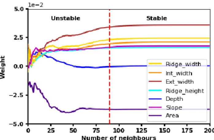
The first step to run the ReliefF algorithm is to set the number of neighbours used to compute the weights. The contributions of the inputs are unstable for a smaller number of neighbours (Fig.7). The smallest number of neighbours for the model to enter the stable weight domain is 90. Next, the ReliefF is run on the whole dataset to obtain the ranking and contribution weight of the parameters. The width parameters are the most pertinent parameters. The three parameters on the podium are the exterior width, the ridge width and the interior width, in descending order of weight. On the contrary, the depth and the area are excluded because parameters with negative weight are irrelevant [9, 13]. Finally, the slope is ranked fourth out of seven parameters, so its contribution with the ReliefF method is limited. However, since the optimal subset is not defined by the ReliefF algorithm, consequently, all the positive weight parameters including the slope are chosen .

Figure 7: Evolution of the ReliefF weights versus the number of neighbours.

Next, the Sequential algorithm is performed in the forward direction. The error is evaluated for all feature combinations to optimize the number of parameters needed to get the most accurate subset to predict and analyse the topic (Fig. 8). The misclassification error is stabilised at 4 features (Fig 8), so which means the other parameters do not continue to provide any more information: either those parameters are irrelevant, or they are correlated to other parameters already used in the subset. With all 7 parameters in the subset, the misclassification error increases again: the last parameter, the area, adds noise in the classification model.

The FSS returns only the optimal subset. Consequently, the model cannot estimate the contribution of each parameter in the subset. To get an outlook on the main contributors, the algorithm was repeated with one parameter each time. This singleton with the slope parameter classifies 81% of scratches. The model progresses to 85% accuracy (Fig.10) with 4 features. The subset is completed with the ridge width, the ridge height and the interior width.

The sequential method analyses all the features together, bringing the interaction of the parameters into play. In this study, the height and the width are analysed together as a new slope parameter. The ratio of the height and the width is approximately the slope, not inside of the scratch but on the ridge that we didn’t compute. In another example, the summation of the ridge width and the interior width are quasi-equal to the exterior width which is the most relevant parameter for the ReliefF algorithm. This might be the reason why the sequential method returns similar parameters to the ReliefF method.

Figure 8: Misclassification error in function of the number feature in the subset modelled by the sequential method.

The embedded method to complete the overview of the classification is the decision tree. The tree classifies the data with 4 parameters: the depth, the exterior width, the interior width and the slope. The classification is the most accurate with less than 10% error (Fig.10) with a short tree without any need to prune the tree. The first two branches containing the depth and exterior width nodes (Fig 9.a) divide the data into four domains (Fig 9.b). In the first domain with wide and deep scratches, the scratches are always visible. Similarly, in the second domain with wide and shallow scratches, the scratches are also visible. Hence, all wide scratches with an exterior width larger than 34.8µm are visible. In the third domain with shallow and narrow scratches, the visibility of the scratches is inconclusive. The scratches can be filtered with the interior width. When the exterior and the interior width of these scratches are almost the same, the slope is quasi-horizontal, and the scratch is invisible. When the interior width is small, the scratches become visible due to their ridges, small and sharp, and the model is able to extract this. The last domain with deep and narrow scratches is the hardest to classify. The most discriminative parameter is the slope but it only splits the data at 60%. Misclassification occurs more frequently in both the visible and invisible prediction due to an uncertainty on the slope limit.

Figure 9: a) A tree developed in the method a decision tree, b) Depth in function of the exterior width, in black the limit defined by the tree

The comparison of the different methods NCA, ReliefF, forward Sequential, and decision tree indicates a similar classification, in particular with the slope or with a width and height parameter combination. The accuracy of the model is the highest for the embedded method with 10% of misclassification, followed by the wrapper method (14.5%) and the filter method (28%). The reason for the smaller misclassification in the embedded and wrapped methods is because these two models analyse the interaction between the features, an important thing in this case due to the height and the width parameter interaction.

Figure 10: Misclassification error in function of the method. 4.3 – Optimal cosmetic classification subset

The Table 3 gathers the contribution of each parameters in function of the method. The feature selection methods excluded only one parameter, the area (Table 3). However, the other parameters can be used due to their physical link with the visibility. An optimal subset is proposed based on 4 features: the slope, the interior and exterior width and the depth.

The feature selection methods expose one main parameter: the slope. This parameter is physically linked to the reflection, the refraction, and the scattering of the light on a surface. The light is reflected from the normal of the surface and consequently the slope and this provides a local description of the surface orientation. It has remained a tricky parameter to manage on a surface because, there, it was measured inside the furrow, so it is a local parameter. It is likely to be one of the sources of the misclassification of the decision tree, or the NCA method, because the most selective slope could not be in the location that this parameter was computed. Hence, this parameter could be improved or optimized by different approaches, like the average of the slope [27], or the Rdq parameter, to improve the robustness of the prediction.

Moreover, it is known that an average human eye can discern a pattern of 90 µm from 30 cm away by a visual angle of 1/60° [24]. This identification is precisely the size of the scratch for the eye resolution and it is correlated with the selected parameters: the interior and the exterior width. Nevertheless, those parameters are relevant because the surface gradient is important on the cross-section. In the scratch direction, the gradient is too low to be pertinent. The interior width could be included even if the rank of this parameter is lower than the others because it is an input of the wrapper method and the embedded method and it can be used to get a more accurate prediction. This parameter is a stabiliser of the prediction for two possible reasons. First, the ratio of the depth to

interior width is an image of the main parameter, the slope. Second, the difference between the interior and the exterior width provides information on ridge width.

Then, to complete the optimal subset, the depth is the final candidate. This parameter is double, it is very selective with the decision tree method, but it was eliminated by all the other methods. In fact, it is not directly linked to the visibility of the scratch, because the depth is spread between 0 and 9µm, higher than the eye resolution. However, the shape of the indenter links the depth to the interior width, and their correlation is high, 0.91 (Pearson coefficient). Thus, the depth correlates with eye resolution due to the its correlation with the width of the scratch. Moreover, the ratio of depth to width is also correlated again to the slope. Nevertheless, these correlations could be made irrelevant in the case of a linear shape or a laser, because the depth would then be independent of the width. Finally, the optimal subset proposed is the same as the decision tree designs (Table 3), and it is confirmed by the other feature selection methods. Those parameters are coherent with the parameters studied for a non-coated polymer surface: the slope and the width of the defect. It confirms also the influence of the initial surface irregularities on the coating flow, even for the shallowest scratches.

Table 3: Summary of the parameter contributions.

5. Conclusion

To conclude, the first observations confirm a similar behaviour of the coating on the increasing scratch and the constant scratch with a same force threshold. Consequently, the morphological parameters in the scratching direction and the scratch length have been excluded from the inputs.

Four feature selection methods were studied to find an optimal subset to control and predict the cosmetic of the MR7 polymer surface after the coating with the surface after the surfacing process. The observations lead to exclude the area and the ridge parameters.

The slope is one of the main parameters. However, the slope is not enough to get a fine prediction as the NCA showed, and the subset should be completed with the exterior width exposed by ReliefF, the decision tree, and the sequential method in the interaction of the ridge width and the interior width. Then, the subset could be optimized with depth and the interior width to have an accurate prediction.

On the other hand, the four methods are necessary to have an overview of the parameter influences, on the classification. In fact, with a single method as a first approach, it’s easy to miss the relevant parameters like the depth only exposed by the decision Tree.

The study could be completed with a feature selection with a regression method to correlate the contrast after the coating to the same morphological parameters. In addition, the subset could be tested on laser scratching, or other speed conditions and on other polymers to validate it or to reinforce the model.

Lastly, the study could be opened on the coating process and the coating itself. In fact, the thickness, the viscosity of the coating or the process are variables which influence the cosmetic of the surface.

References

[1] M. El Mansori, S. Mezghani, H. Zahouani, F. Divo, Biomimetic touch perception of edge finish of ophthalmic lens, Wear, Volume 301, Issue 1-2, 362-369

[2] S. Mezghani, H. Zahouani, J.-J. Piezanowski, Multiscale characterizations of painted surface appearance by continuous wavelet transform, Journal of Materials Processing Technology, Volume 211, Issue 2, Pages 205-211 [3] S. Bessonnet, M. El Mansori, S. Mezghani, S. Pinault, Multi-scale computation of multistage manufacturing process signatures of glassy polymers multi-functionalisation, Procedia Manufacturing, Volume 26, Pages 681-689 [4] M. Gamble, S. Mezghan, M. El Mansori, F. Divo, Interferometric and microscopic measurements of surface finish appearance evaluations of ophthalmic lens edges, AIP Conference Proceedings Volume 1315, Issue 1, Pages 1353-1358

[5] M. Rebsamen, J-M. Boucheix, and M. Fayol. Quality control in the optical industry: From a work analysis of lens inspection to a training programme, an experimental case study. Applied Ergonomics, Volume 41, Issue 1, Pages 150-160, 2010.

[6] P. Kurkcu, L. Andena, A. Pavan, An experimental investigation of the scratch behaviour of polymers: 1. Influence of rate-dependent bulk mechanical properties, Wear, Volume 290–291, Pages 86–93, 2012

[7] A. Jović, K. Brkić and N. Bogunović, A review of feature selection methods with applications, Information and Communication Technology Electronics and Microelectronics (MIPRO) 2015 38th International Convention, Pages 1200-1205, 2015

[8] Y. Saeys, I. Inza and P. Larrañaga, A review of feature selection techniques in bioinformatics, Bioinformatics, Volume 23, Issue 19, Pages 2507–2517, 2007

[9] R. J. Urbanowicza, M. Meekerb, W. LaCavaa, R. S. Olsona, J. H. Moore Relief-Based Feature Selection: Introduction and Review, Biomedical Informatics, 2018

[10] V. Kumar and S. Minz, Feature Selection: A literature Review, Smart Computing Review, Volume 4, Issue 3, 2014

[11] C. Ding and H. Peng, Minimum Redundancy Feature Selection from Microarray Gene Expression Data, Journal of Bioinformatics and Computational Biology, Volume 03, Issue 02, Pages 185-205, 2005

[12] Theoretical and Empirical Analysis of ReliefF and RReliefF, Machine Learning, Volume 53, Issue 1–2, pp 23– 69, 2003

[13] K. Kira and L. A. Rendell, A practical approach to feature selection, ML92 Proceedings of the ninth international workshop on Machine learning, Pages 249-256, 1992

[14] K. Dunne, P. Cunningham, F. Azuaje, Solutions to Instability Problems with Sequential Wrapper-based Approaches to Feature Selection, Journal of Machine Learning Research, 2002

[15] W. Yang, K. Wang and W. Zuo, Neighborhood Component Feature Selection for High-Dimensional Data. Journal of Computers. Volume 7, Issue 1, Pages 161-168, 2012.

[16] W. Yang, K. Wang and W. Zuo, Fast neighborhood component analysis, Neurocomputing, Volume 83, Pages 31-37, 2012

[17] I. Kononenko, E. Simec, M. Robnik-Sikonj, Overcoming the myopia of inductive algorithms with RELIEFF, Applied Intelligence, Volume 7, Issue 1, Pages 39–55, 1997

[18] T. Waheed, R. B. Bonnell, S. O. Prasher, E. Paulet, Measuring performance in precision agriculture: CART— A decision tree approach, Agricultural Water Management, Volume 84, Issues 1–2, Pages 173-185, 2006

[19] Breiman L, Friedman JH, Olshen RA, Stone CJ. Classification and Regression Trees. Belmont California: Wadsworth, Inc.; 1984

[20] H. Pelletier, C. Gauthier, R. Schirrer, Comportement à la rayure de surfaces de polymères : comparaison entre mesures expérimentales et simulations numériques, 18ème Congrès Français de Mécanique, 2007

[21] H. Pelletier, C. Gauthier, R. Schirrer Relationship between contact geometry and average plastic strain during scratch tests on amorphous polymers, Tribology International, Volume 43, Pages 796–809, 2010

[22] H. Pelletier, A.-L. Durier, C. Gauthier, R. Schirrer Viscoelastic and elastic– plastic behaviors of amorphous polymeric surfaces during scratch, Tribology International, Volume 41, Pages 975– 984, 2008

[23] H. Jianga, R. L. Browninga, M. M. Hossaina, H.-J. Suea, M. Fujiwarab, Quantitative evaluation of scratch visibility resistance of polymers, Applied Surface Science, Volume 256, Pages 6324–6329, 2010

[24] C. J. Barr1, L. Wang, J. K. Coffey, and F. Daver, Influence of surface texturing on scratch/mar visibility for polymeric materials: a review, Journal of Materials Science, Volume 52, Issue 3, Pages 1221–1234, 2017

[25] J. Zhang, H. Jiang, C. Jiang, Q. Cheng, G. Kang, In-situ observation of temperature rise during scratch testing of poly(methylmethacrylate) and polycarbonate, Tribology International, Volume 95, Pages 1–4, 2016

[26] H. Jiang, R. Browning, H. Sue, Understanding of scratch-induced damage mechanisms in polymers, Polymer, Volume 50, Pages 4056–4065, 2009

[27] M. Hamdi, H-J. Sue, Effect of color, gloss, and surface texture perception on scratch and mar visibility in polymers. Materials and Design Volume 83, Pages 528–535, 2015