HAL Id: tel-03073054
https://pastel.archives-ouvertes.fr/tel-03073054
Submitted on 16 Dec 2020
HAL is a multi-disciplinary open access
archive for the deposit and dissemination of sci-entific research documents, whether they are pub-lished or not. The documents may come from teaching and research institutions in France or abroad, or from public or private research centers.
L’archive ouverte pluridisciplinaire HAL, est destinée au dépôt et à la diffusion de documents scientifiques de niveau recherche, publiés ou non, émanant des établissements d’enseignement et de recherche français ou étrangers, des laboratoires publics ou privés.
permanent magnet synchronous machine drives under
constraints on current and voltage for automotive
applications
Duc Tan Vu
To cite this version:
Duc Tan Vu. Fault-tolerant control of non-sinusoidal multiphase permanent magnet synchronous machine drives under constraints on current and voltage for automotive applications. Electric power. HESAM Université, 2020. English. �NNT : 2020HESAE040�. �tel-03073054�
ÉCOLE DOCTORALE SCIENCES DES MÉTIERS DE L’INGÉNIEUR
[L2EP – Campus de Lille]
THÈSE
présentée par :
Duc Tan VU
soutenue le : 24 novembre 2020
pour obtenir le grade de : Docteur d’HESAM Université
préparée à :
École Nationale Supérieure d’Arts et Métiers
Spécialité : Génie électrique
Fault-tolerant control of non-sinusoidal
multiphase permanent magnet synchronous
machine drives under constraints on current
and voltage for automotive applications
THÈSE dirigée par :[M. Eric SEMAIL] et co-encadrée par : [M. Ngac Ky NGUYEN]
Jury
M. Mohamed BENBOUZID, Professeur des universités, IRDL, Université de Bretagne Occidentale Président
M. Franck BETIN, Professeur des universités, LTI, Université de Picardie Jules Verne Rapporteur
M. Johan GYSELINCK, Professeur des universités, BEAMS, Université Libre de Bruxelles Rapporteur
Mme. Carole HENAUX, Maître de conférences HDR, LAPLACE-UPS-INPT, Université de Toulouse Examinatrice
M. Eric SEMAIL, Professeur des universités, L2EP, Arts et Métiers Sciences et Technologies/ENSAM Examinateur
M. Ngac Ky NGUYEN, Maître de conférences, L2EP, Arts et Métiers Sciences et Technologies/ENSAM Examinateur
T
H
È
S
E
i
Acknowledgments
This thesis has been carried out for three years and nine months, under the supervision of M. Eric SEMAIL and M. Ngac Ky NGUYEN. I can say that I am a very lucky student as my supervisors have been always available for discussions regardless of their busy schedules. Thus, there are a lot of things that I have learned from them. Without their support, I would not have been able to finish this research. I do not think that I could have found better supervisors for my PhD study. Therefore, I would like to express my special gratitude to M. Eric SEMAIL and M. Ngac Ky NGUYEN for their guidance, support, patience, and encouragement.
I would like to acknowledge the jury of my thesis defense. Despite the pandemic, all members of the jury have spent their time to give me their insightful comments and hard questions which have incented me to widen my research from various perspectives. I would like to thank M. Mohamed BENBOUZID, professor at Université de Bretagne Occidentale, France for being the president of the jury. I would like to thank M. Franck BETIN, professor at Université de Picardie Jules Verne, France, and M. Johan GYSELINCK, professor at Université Libre de Bruxelle, Belgium for being the reviewers of my thesis. I would like to thank Mme. Carole HENAUX, associate professor at Université de Toulouse, France for being the examiner of my thesis.
I would like to thank M. Alain BOUSCAYROL, head of the control team in L2EP laboratory for his valuable advice. I would like to thank Mme. Betty SEMAIL, director of L2EP laboratory, for her support from my early days in the laboratory. I also would like to thank all professors, colleagues, and staffs of L2EP as well as those at ENSAM, including laboratories LISPEN and LMFL.
I would like to express my gratitude to the Ministry of Education and Training, a representative of the Vietnamese government, for the four-year scholarship. I also would like to thank Campus France, a representative of the French government, together with ENSAM and CE2I project for their valuable support. My sincere thanks go to my dear colleagues at Thai Nguyen University of Technology for favorable conditions enabling me to pursue my PhD study.
I have experienced one of the most memorable periods in my life, as a PhD student, thanks to my wonderful friends. I am thankful to anh Kỳ, chị Xiaoxiao, Noé, Thùy Anh, Hai Long, anh Long, chị Thủy, anh Châu, Bảo Huy, Chi, Tiago, Hussein, Youssouf, Jinlin, Lamine, Keitaro, and all members of football team Les Ch’tis.
Last but not least, my profound gratitude goes to my family for supporting me unconditionally. This thesis is dedicated to my family, including my grandparents, my parents, my brothers, my sisters, especially my wife Vân Anh and my little daughter Hoàng Mai.
iii
Abstract
The electrification of transportation has been considered as one of solutions to tackle the shortage of fossil energy sources and air pollution. Electric drives for electrified vehicles, including pure electric and hybrid electric vehicles, need to fulfil some specific requirements from automotive markets such as high efficiency, high volume power and torque densities, low-cost but safe-to-touch, high functional reliability, high torque quality, and flux-weakening control. In this context, multiphase permanent magnet synchronous machine (PMSM) drives have become suitable candidates to meet the above requirements.
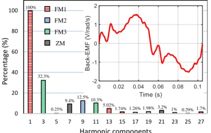
The main objective of this doctoral thesis is to propose and refine fault-tolerant control strategies for non-sinusoidal multiphase PMSM drives that require less constraints on their design. In addition, constraints on current and voltage defined by the inverter and the machine are considered to optimize the machine control under the non-sinusoidal condition without exceeding their allowable limits. Therefore, the system sizing is guaranteed, especially in flux-weakening operations. The proposed fault-tolerant control strategies, based on the mathematical model of multiphase drives, enrich the control field of multiphase drives by providing various control options. The selection of one of the proposed control options can be a trade-off between a high quality torque but a low average value and a high average torque but a relatively high ripple. The control and torque performances of the drives can be refined by using artificial intelligence with a simple type of artificial neural networks named ADALINE (ADAptive LInear NEuron). With self-learning ability, fast convergence, and simplicity, ADALINEs can be applied to industrial multiphase drives. All proposed control strategies in this doctoral thesis are validated with an experimental seven-phase PMSM drive. The non-sinusoidal back electromotive force (back-EMF) of the experimental seven-phase PMSM is complex with the presence of multi-harmonics. Experimental results verify the effectiveness of the proposed strategies, and their applicability in a multiphase machine with a complex non-sinusoidal back-EMF.
Keywords: Multiphase machine, seven-phase machine, non-sinusoidal back-EMF,
fault-tolerant control, optimal control under constraint, artificial intelligence, adaptive linear neuron, ADALINE.
v
Résumé
L'électrification des transports a été considérée comme l'une des solutions pour lutter contre la pénurie de sources d'énergie fossile et la pollution de l'air. Les entraînements électriques pour les véhicules électrifiés, y compris les véhicules électriques purs et électriques hybrides, doivent répondre à certaines exigences spécifiques des marchés automobiles, tels qu'un rendement élevé, des densités volumiques élevées de puissance et de couple, un coût faible avec une protection contre les risques électriques, une fiabilité fonctionnelle élevée, une qualité de couple élevée, et un contrôle de défluxage. Dans ce contexte, les entraînements de machines synchrones à aimants permanents (PMSM) polyphasées sont devenus des candidats appropriés pour répondre aux exigences citées ci-dessus.
L’objectif principal de cette thèse de doctorat vise à proposer et affiner des stratégies de commandes tolérantes aux défauts pour les entraînements de machines PMSM polyphasées non-sinusoïdales qui requièrent moins de contraintes lors de leur conception. Par ailleurs, les contraintes de courant et de tension définies par l’onduleur et la machine sont prises en compte pour optimiser en régime non-sinusoïdal le contrôle de la machine sans dépasser les limites admissibles. Cela permet idéalement un dimensionnement au plus juste et cela tout particulièrement dans la zone de défluxage. Les stratégies proposées de commandes tolérantes aux défauts, basées sur le modèle mathématique des entraînements polyphasés, enrichissent le domaine de contrôle des entraînements polyphasés en offrant de diverses options de contrôle. Le choix de l'une des options proposées de commande peut être un compromis entre un couple de haute qualité mais avec une valeur moyenne faible, et un couple moyen élevé mais avec une ondulation relativement élevée. Les performances de contrôle et de couple peuvent être affinées en utilisant l'intelligence artificielle avec un type simple de réseaux de neurones artificiels nommé ADALINE (neurone linéaire adaptatif). Grâce à leur capacité d'auto-apprentissage, à leur convergence rapide, et à leur simplicité, les ADALINE peuvent être appliqués aux entraînements polyphasés industriels. Toutes les stratégies de contrôle proposées dans cette thèse de doctorat sont validées avec un entraînement d’une machine PMSM à sept phases. La force électromotrice non-sinusoïdale de la machine PMSM à sept phases, relevée expérimentalement, est complexe avec la présence de plusieurs harmoniques. Les résultats expérimentaux vérifient l'efficacité des stratégies proposées, et leur applicabilité dans une machine polyphasée avec une force électromotrice non-sinusoïdale complexe.
Mots clés : Machine polyphasée, machine à sept phases, force électromotrice non-sinusoïdale,
commande tolérante aux défauts, commande optimale sous contrainte, intelligence artificielle, neurone linéaire adaptatif, ADALINE.
vii
Contents
Acknowledgments ... i Abstract ... iii Résumé ... v Nomenclature ... xiList of figures ... xvi
List of tables ... xxv
Introduction ... 1
Chapter 1. Multiphase Drives: Opportunities and State of the Art ... 5
1.1. Multiphase drives for automotive applications ... 5
Multiphase drives: a suitable candidate for EVs ... 5
1.1.1.A. Low power per phase rating for safe EVs ... 6
1.1.1.B. Fault-tolerant ability for high functional reliability ... 6
1.1.1.C. Low ripple torques for smooth EVs ... 7
1.1.1.D. More possibilities of stator winding configurations ... 8
1.1.1.E. Electromagnetic pole changing by imposing harmonics of current ... 8
Opportunities for multiphase drives in automotive applications ... 9
Recent projects on multiphase drives ... 11
1.1.3.A. MotorBrain project ... 11
1.1.3.B. CE2I project ... 12
Section summary ... 12
1.2. General model of a multiphase PMSM ... 12
Natural frame model ... 13
Decoupled stator reference frame model ... 13
Rotor reference frame model ... 15
1.3. State of the art in the control field of multiphase drives ... 16
Existing control techniques of multiphase drives in healthy mode ... 16
1.3.1.A. FOC ... 16
1.3.1.B. DTC ... 18
1.3.1.C. MPC ... 19
viii
1.3.2.A. Possible faults in multiphase drives ... 20
1.3.2.B. Categorization based on criteria of new current references for fault-tolerant operations ... 21
1.3.2.C. Categorization based on types of MMFs for fault-tolerant operations ... 21
1.3.2.D. Categorization based on modeling of multiphase drives for fault-tolerant operations ... 22
1.3.2.E. Categorization based on control techniques for fault-tolerant operations ... 22
1.4. Objectives of the doctoral thesis ... 23
1.5. Conclusions ... 25
Chapter 2. Modeling and Control of Multiphase Drives ... 27
2.1. Modeling and control of a multiphase drive in healthy mode... 27
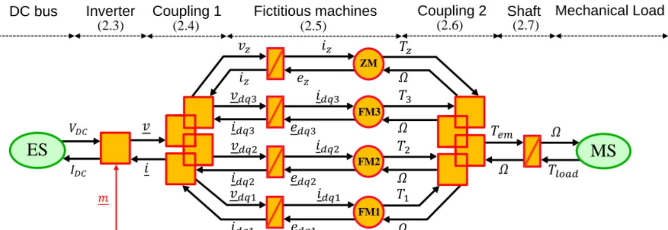
The case study: a seven-phase PMSM ... 27
Energetic Macroscopic Representation for modeling and control ... 29
2.1.2.A. The representation of the electric drive model ... 29
2.1.2.B. The representation of the electric drive control ... 32
Control scheme with an optimal control strategy under constraints on RMS current and peak voltage in healthy mode ... 34
Control performances of a seven-phase PMSM drive in healthy mode ... 36
2.1.4.A. Assumptions and experimental setup descriptions ... 36
2.1.4.B. Optimal calculations under constraints on RMS current and peak voltage .... 38
2.1.4.C. Verification with experimental results for healthy mode ... 39
2.2. Control of a multiphase drive in an OC fault without reconfigurations ... 44
An OC fault in a seven-phase PMSM drive ... 44
Control performances in an OC fault without reconfigurations ... 45
2.2.2.A. Current control performance ... 45
2.2.2.B. Torque performance ... 46
2.2.2.C. Constraints on RMS current ... 46
2.2.2.D. Comparative summary ... 47
2.3. Fault-tolerant control for a multiphase drive ... 48
Introduction to proposed fault-tolerant control methods ... 48
Method (I): new current references determined from decoupled reference frames 50 2.3.2.A. Principle of method (I) ... 50
ix
2.3.2.B. Method (I)-1 ... 53
2.3.2.C. Method (I)-2 ... 53
2.3.2.D. Method (I)-3 ... 54
2.3.2.E. Comparative analyses of calculated results by the proposed options of method (I) ... 55
2.3.2.F. Verification with experimental results for method (I) ... 60
Method (II): new current references determined from reduced-order transformation matrices ... 65
2.3.3.A. Principle of method (II) ... 65
2.3.3.B. Method (II)-RCA (Robust Control Approach) ... 69
2.3.3.C. Method (II)-SCL (Similar Copper Losses) ... 69
2.3.3.D. Summary of current design options in method (II) ... 71
2.3.3.E. Comparative analyses of calculated results with methods RCA and (II)-SCL ... 72
2.3.3.F. Verification with experimental results for method (II) ... 75
Method (III): new current references determined from natural frame ... 80
2.3.4.A. Principle of method (III)... 80
2.3.4.B. Sinusoidal phase currents for sinusoidal back-EMFs ... 81
2.3.4.C. Sinusoidal phase currents for non-sinusoidal back-EMFs ... 83
2.3.4.D. Non-sinusoidal phase currents for non-sinusoidal back-EMFs ... 85
2.3.4.E. Summary of current design options in method (III) ... 90
2.3.4.F. Comparative analyses of calculated results with methods (III)-1 and (III)-2 . 90 2.3.4.G. Verification with experimental results for method (III) ... 93
Comparative analyses of fault-tolerant control methods (I), (II) and (III) ... 98
2.3.5.A. Comparisons in terms of control facilitation ... 98
2.3.5.B. Comparisons in terms of torque, copper loss, and speed range ... 98
2.3.5.C. Comparisons of three remarkable methods using radar charts ... 100
2.3.5.D. Comparisons with recent studies ... 101
2.4. Conclusions ... 101
Chapter 3. Enhancements of Multiphase Drive Performances with Adaptive Linear Neurons ... 103
x
Artificial neural networks and adaptive linear neurons ... 103
Possible applications of ADALINEs in the electric drive ... 105
3.2. Control quality in healthy mode ... 105
Impacts of unwanted back-EMF harmonics and the inverter nonlinearity ... 106
3.2.1.A. Impacts of unwanted back-EMF harmonics ... 106
3.2.1.B. Impacts of the inverter nonlinearity ... 107
3.2.1.C. Summary of the impacts of unwanted back-EMF harmonics and the inverter nonlinearity ... 108
Eliminations of current harmonics in rotating frames ... 109
3.2.2.A. The conventional control scheme with the back-EMF compensation ... 109
3.2.2.B. The proposed control scheme to eliminate current harmonics in rotating frames ... 109
3.2.2.C. Verification with experimental results ... 111
3.2.2.D. Torque performance after eliminating current harmonics in rotating frames ... 114
Direct eliminations of torque ripples in healthy mode ... 115
3.2.3.A. The proposed control scheme to directly eliminate torque ripples in healthy mode ... 115
3.2.3.B. Comparisons with the vectorial approach by real-time simulation results ... 116
3.2.3.C. Verification with experimental results ... 118
3.3. Control quality in faulty mode ... 122
Direct eliminations of torque ripples in faulty mode with method (III)-2 ... 122
3.3.1.A. Harmonic components of torque and the proposed control structure... 122
3.3.1.B. Verification with experimental results ... 123
Current control improvements in faulty mode with method (II)-RCA ... 126
3.3.2.A. Time-variant current references ... 126
3.3.2.B. Proposed control structure to use time-constant d-q current references ... 127
3.3.2.C. Verification with experimental results ... 130
3.4. Conclusions ... 133
General conclusions and Perspectives ... 135
References ... 138
xi
Nomenclature
Abbreviations
AC Alternating Current
ADALINE ADAptive LInear NEuron
AI Artificial Intelligence
ANN Artificial Neural Network
BEV Battery Electric Vehicle
CBPWM Carrier Based Pulse Width Modulation
CCS-MPC Continuous Control Set Model-based Predictive Control
CE2I The Intelligent Integrated Energy Converter project
DC Direct Current
DoF Degrees of Freedom
DTC Direct Torque Control
EMF Electromotive Force
EMR Energetic Macroscopic Representation
ES Electrical Source
est, est estimated
EV Electrified Vehicle
exp, exp experimental or experiment
FCV Fuel Cell Vehicle
FL Fuzzy Logic
FM Fictitious Machine
FOC Field-Oriented Control
FS-MPC Finite Set Model-based Predictive Control
HEV Hybrid Electric Vehicle
HM Healthy Mode
ICE Internal Combustion Engine
IGBT Insulated-Gate Bipolar Transistor
IM Induction Machine
xii
LMS Least Mean Square
mea, mea measured
MMF Magnetomotive Force
MPC Model-based Predictive Control
MS Mechanical Source
MTPA Maximum Torque Per Ampere
OC Open Circuit
opt, opt optimal or optimization
PI Proportional Integral
PIR Proportional Integral Resonant
PMSM Permanent Magnet Synchronous Machine
pu per unit
PWM Pulse Width Modulation
PWM-DTC Pulse Width Modulation Direct Torque Control
RCA Robust Control Approach
ref, ref reference
RMS Root Mean Square
SC Short Circuit
SCL Similar Copper Losses
ST-DTC Switching Table Direct Torque Control
SVPWM Space Vector Pulse Width Modulation
VSI Voltage Source Inverter
ZM Zero-sequence Machine
Parameters, variables, matrices, and vectors
T
Clarkefault
7-by-6 Clarke transformation matrix when phase A is opened
TClarke1
,
TPark1
6-by-6 new Clarke and Park matrices for the first harmonic of current
TClarke3
,
TPark3
6-by-6 new Clarke and Park matrices for the third harmonic of current[L] n-by-n inductance matrix in natural frame
xiii
[Lαβ] n-by-n inductance matrix in the decoupled stator reference (α-β) frames
[TClarke] n-by-n Clarke transformation matrix
[TPark] n-by-n Park transformation matrix
∆T Torque ripple
A, B, C, D, E, F, G Names of phases of a 7-phase machine
e n-dimensional back-EMF vector in natural frame
edq n-dimensional back-EMF vector in the rotor reference (d-q) frames
edqj 2-dimensional back-EMF vector of two-phase fictitious machine j in the
rotor reference (d-q) frames
En1, En3 Amplitudes of the first and third harmonics of a speed-normalized back-EMF in natural frame, respectively
enA…enG Speed-normalized back-EMFs of phases A to G
Ey The squared error of the ADALINE output
eαβ n-dimensional back-EMF vector in the decoupled stator reference (α-β)
frames
fm Friction coefficient of the rotor load bearings
i n-dimensional phase current vector in natural frame
IDC DC-bus current
idq n-dimensional current vector in the rotor reference (d-q) frames
idqj 2-dimensional current vector of two-phase fictitious machine j in the rotor reference (d-q) frames
Ipeak_lim Limit of the peak phase currents
IRMS Highest RMS current among all phases
IRMS_j RMS current of phase j
IRMS_lim Limit of the RMS phase currents
iαβ n-dimensional current vector in the decoupled stator reference (α-β)
frames
J Cost function in MPC
Jm Moment of inertia of the electric drive and mechanical load
kR Repartition coefficient vector
L Self-inductance of one phase
xiv
L2 Inductance of the second fictitious machine
L3 Inductance of the third fictitious machine
Lz, Lz1, Lz2 Inductances of the zero-sequence machines
M1 Mutual inductance between two phases shifted an angle of 2π/n
M2 Mutual inductance between two phases shifted an angle of 4π/n
M3 Mutual inductance between two phases shifted an angle of 6π/n
n The number of phases of an electric machine
ℕ, ℕ0 Sets of natural numbers without zero and with zero
p Number of pole pairs
Pem Output mechanical power
Ploss Total copper loss
Rs Stator winding resistance of one phase
s Laplace operator
sj, s̅j Switches of leg j of an inverter,
𝑠1,n Switching signal vector for n phases
t Time
T1 Torque of the first fictitious machine
T2 Torque of the second fictitious machine
T3 Torque of the third fictitious machine
Tave Average torque
Tem Electromagnetic torque
Tem_exp Experimental electromagnetic torque
Tem_opt Optimal electromagnetic torque from the offline optimizations
Tload Load torque
Tz Torque of the zero-sequence machine
v n-dimensional phase voltage vector in natural frame
VDC DC-bus voltage
vdq n-dimensional voltage vector in the rotor reference (d-q) frames
vdqj 2-dimensional voltage vector of two-phase fictitious machine j in the rotor reference (d-q) frames
xv
Vlim Limit of the peak phase voltages in experiments
Vlim_opt Limit of the peak phase voltages for the offline optimization
Vpeak Highest peak phase voltage among all phases
vαβ n-dimensional voltage vector in the decoupled stator reference (α-β)
frames
w Weight vector of an ADALINE
wk The kth weight of an ADALINE
x A general n-dimensional vector of machine parameters in natural frame
x One of machine parameters (current i, back-EMF e, or voltage v), or one
of axes (d1, q1, d9, q9, d3, q3) in d-q frames
xdq A general n-dimensional vector of machine parameters in the rotor
reference (d-q) frames
xin Input vector of an ADALINE
xink The kth input of an ADALINE
xαβ A general n-dimensional vector of machine parameters in the decoupled
stator reference (α-β) frames
y Output of an ADALINE
δ Spatial angular displacement of two adjacent phases (equal to 2π/n for a
n-phase machine)
η Learning rate of an ADALINE
θ Electrical position
Ω Rotating speed
Ωbase Base speed
Ωmax Maximum speed
xvi
List of figures
Fig. 1.1. A n-phase machine fed by a n-leg VSI in an EV. ... 5
Fig. 1.2. Different possibilities of stator winding configurations for five-phase machines: star (a), pentagon (b), pentacle (c), and corresponding torque-speed characteristics (d) [45, 46]. ... 8
Fig. 1.3. Electromagnetic pole changing in multiphase drives for speed range extensions: p pole pairs (a), a combination of p and 3p pole pairs (b), and a more general case (c). ... 9
Fig. 1.4. The highly compact electric motor prototype without using rare earth metals in MotorBrain project [58] (a), and the model of an integrated machine in CE2I project [59] (b). ... 11
Fig. 1.5. The schematic diagram of a n-phase multiphase PMSM... 12
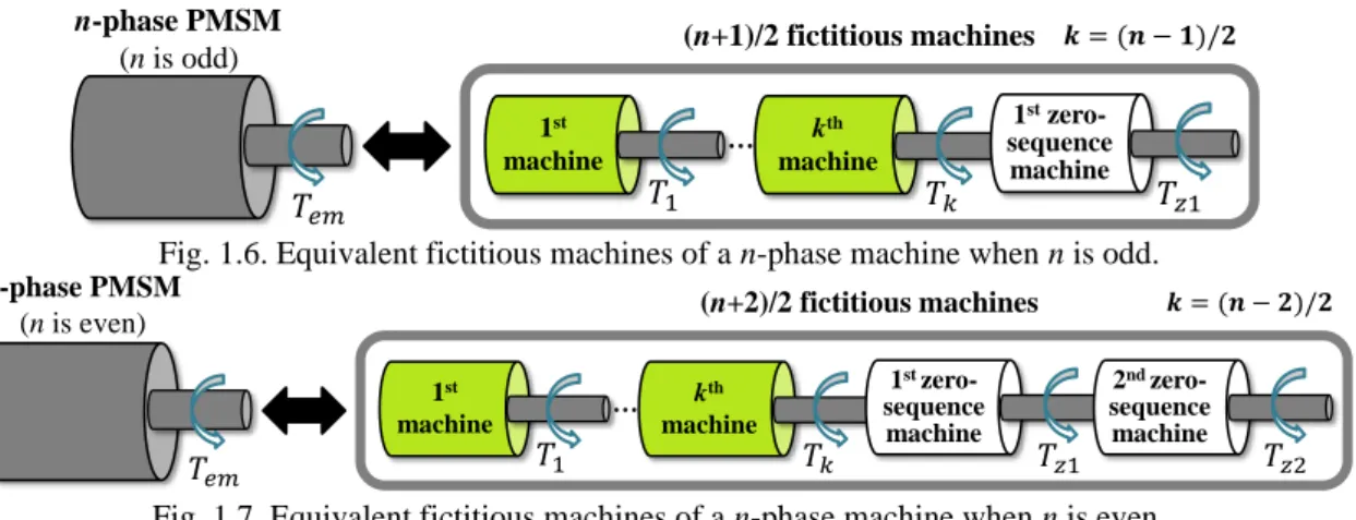
Fig. 1.6. Equivalent fictitious machines of a n-phase machine when n is odd. ... 14
Fig. 1.7. Equivalent fictitious machines of a n-phase machine when n is even. ... 14
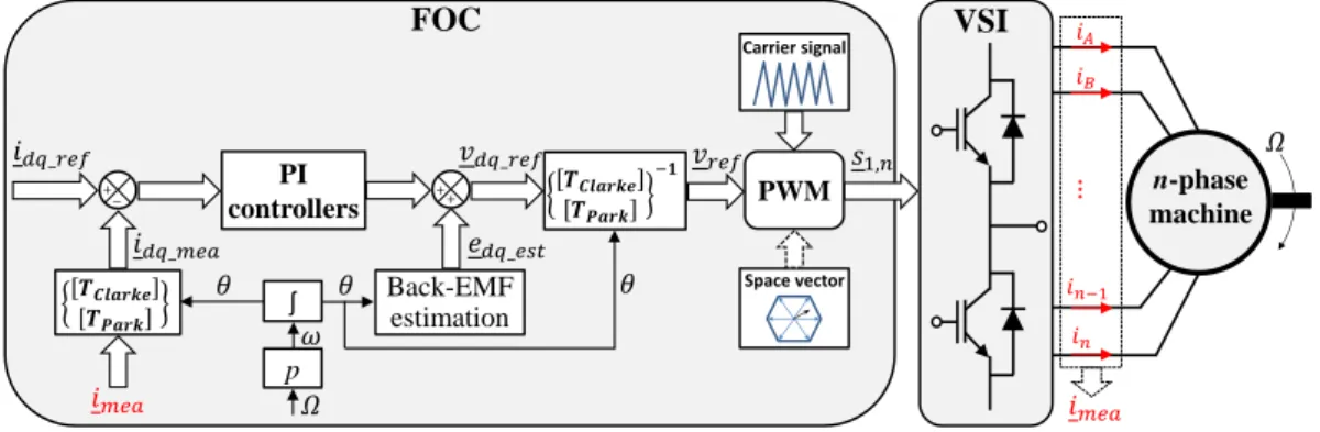
Fig. 1.8. The inner control loop of a n-phase PMSM drive based on FOC technique. ... 17
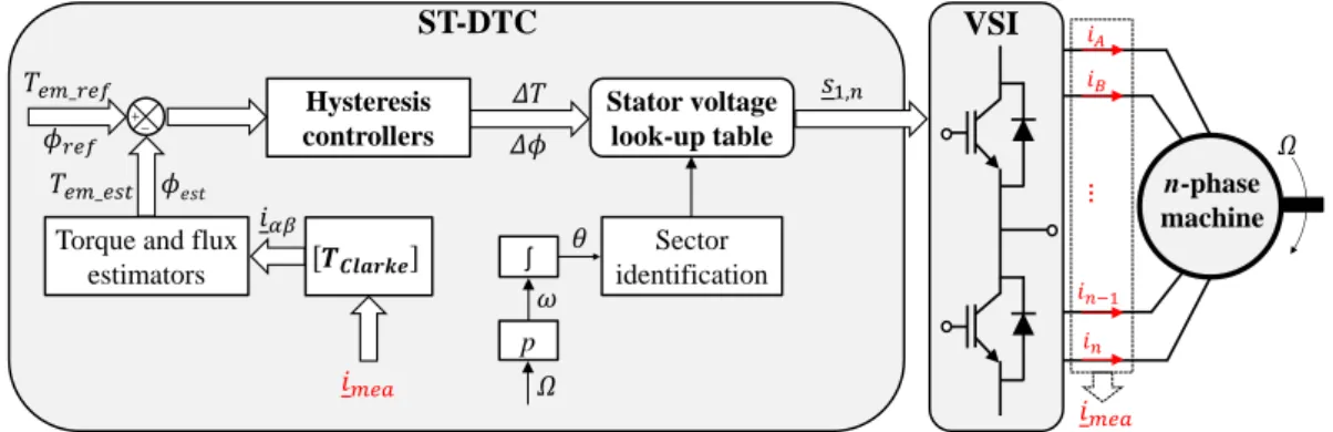
Fig. 1.9. The inner control loop of a n-phase PMSM drive based on ST-DTC technique. ... 18
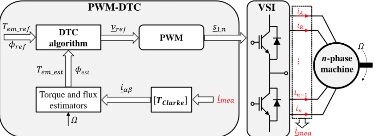
Fig. 1.10. The inner control loop of a n-phase PMSM drive based on PWM-DTC technique. ... 19
Fig. 1.11. The inner control loop of a n-phase PMSM drive based on FCS-MPC technique. . 19
Fig. 1.12. Different types of faults in a n-phase drive. ... 20
Fig. 1.13. Multiphase drives in EVs with two driving modes. ... 24
Fig. 2.1. Schematic diagram of a seven-phase PMSM. ... 27
Fig. 2.2. Decomposition of a seven-phase machine into four fictitious machines. ... 29
Fig. 2.3. Representation of the model of a seven-phase PMSM drive using EMR. ... 30
Fig. 2.4. The general control scheme of a seven-phase PMSM drive with speed and current control represented by EMR. ... 32
Fig. 2.5. The control scheme of a seven-phase PMSM drive with current control represented by EMR. ... 34
Fig. 2.6. The control scheme of a seven-phase PMSM drive in healthy mode with the optimal control strategy under constraints on RMS current and peak voltage, represented by EMR. ... 36
Fig. 2.7. Experimental test bench of the seven-phase PMSM drive. ... 37
Fig. 2.8. The measured speed-normalized back-EMF and harmonic spectrum of the experimental seven-phase PMSM. ... 38
xvii
Fig. 2.9. (Calculated result) Optimal torque-speed characteristic (a), all RMS phase currents (b), and all peak phase voltages (c) in terms of speed under constraints on RMS current and peak voltage in healthy mode. ... 39 Fig. 2.10. (Experimental result) Currents in (d1-q1) frame in terms of time at 20 rad/s with id1_ref=0 A and iq1_ref=12.7 A (a), and in terms of speed (b) in healthy mode. ... 39 Fig. 2.11. (Experimental results) Currents in (d9-q9) frame in terms of time at 20 rad/s with id9_ref=0 A and iq9_ref=1.6 A (a), and in terms of speed (b) and in healthy mode. ... 40 Fig. 2.12. (Experimental result) Currents in (d3-q3) frame in terms of time at 20 rad/s with id3_ref=0 A and iq3_ref=4.1 A (a), and in terms of speed (b) in healthy mode. ... 40 Fig. 2.13. (Experimental result) Torques in terms of time at 20 rad/s (a), and torque-speed characteristics (b) in healthy mode. ... 41 Fig. 2.14. (Experimental result) Phase currents in terms of speed, and current waveforms at 20 and 55 rad/s in healthy mode. ... 42 Fig. 2.15. (Experimental result) Phase voltage references in terms of speed, and voltage reference waveforms at 20 and 55 rad/s in healthy mode. ... 42 Fig. 2.16. An OC fault happens in phase A of a seven-phase PMSM drive. ... 44 Fig. 2.17. (Experimental result) Measured currents in (d1-q1) frame (a), (d9-q9) frame (b), and (d3-q3) frame (c) when phase A is open-circuited without any reconfigurations at 20 rad/s. ... 45 Fig. 2.18. (Experimental result) Torques in healthy mode and when phase A is open-circuited without any reconfigurations at 20 rad/s. ... 46 Fig. 2.19. (Experimental result) Measured phase currents in healthy mode (a), and when phase A is open-circuited without any reconfigurations (b), at 20 rad/s. ... 46 Fig. 2.20. General scheme of the proposed fault-tolerant control methods when phase A is open-circuited. ... 49 Fig. 2.21. The control scheme of a seven-phase PMSM drive for faulty modes with an optimal control strategy under constraints on current and voltage, represented by EMR. ... 50 Fig. 2.22. Desired currents (iα1, iβ1, iα3, iβ3) (a), and (id1, iq1, id3, iq3) (b), at 20 rad/s with (id1=0 A, iq1=12.7 A, id3=0 A, iq3=4.1 A). ... 51 Fig. 2.23. Circles created by desired currents (iα1, iβ1) (a), and (iα3, iβ3) (b). ... 51 Fig. 2.24. Desired currents (iα2, iβ2, iz) (a), currents (id9, iq9, iz) (b), and phase currents (c), at 20 rad/s with method (I)-1 for an OC fault in phase A to preserve the healthy-mode torque (id1=0 A, iq1=12.7 A, id3=0 A, iq3=4.1 A)... 56 Fig. 2.25. Desired currents (iα2, iβ2, iz) (a), currents (id9, iq9, iz) (b), and phase currents (c), at 20 rad/s with method (I)-2 for an OC fault in phase A to preserve the healthy-mode torque (id1=0 A, iq1=12.7 A, id3=0 A, iq3=4.1 A)... 56
xviii
Fig. 2.26. Desired currents (iα2, iβ2, iz) (a), currents (id9, iq9, iz) (b), and phase currents (c), at 20 rad/s with method (I)-3 for an OC fault in phase A to preserve the healthy-mode torque (id1=0 A, iq1=12.7 A, id3=0 A, iq3=4.1 A)... 56 Fig. 2.27. Desired currents (iα2, iβ2, iz) (a), currents (id9, iq9, iz) (b), and phase currents (c), at 20 rad/s with method (I)-1 for an OC fault in phase A under constraints on RMS current and peak voltage (id1=0 A, iq1=6.4 A, id3=0 A, iq3=3.2 A). ... 58 Fig. 2.28. Desired currents (iα2, iβ2, iz) (a), currents (id9, iq9, iz) (b), and phase currents (c), at 20 rad/s with method (I)-2 for an OC fault in phase A under constraints on RMS current and peak voltage (id1=0 A, iq1=7.9 A, id3=0 A, iq3=3.8 A). ... 58 Fig. 2.29. Desired currents (iα2, iβ2, iz) (a), currents (id9, iq9, iz) (b), and phase currents (c), at 20 rad/s with method (I)-3 for an OC fault in phase A under constraints on RMS current and peak voltage (id1=0 A, iq1=7.9 A, id3=0 A, iq3=0.5 A). ... 58 Fig. 2.30. (Calculated result) Optimal post-fault torque-speed characteristics (a), all RMS phase currents (b) and all peak phase voltages (c), in terms of speed under constraints on RMS current and peak voltage with methods (I)-1, (I)-2, and (I)-3 when phase A is open-circuited. ... 59 Fig. 2.31. (Experimental result) Currents in (d1-q1) frame in terms of speed with method (I)-2 (a), and with method (I)-3 (b), when phase A is open-circuited. ... 61 Fig. 2.32. (Experimental result) Currents in (d3-q3) frame in terms of speed with method (I)-2 (a), and with method (I)-3 (b), when phase A is open-circuited. ... 61 Fig. 2.33. (Experimental results) Currents in (d9-q9) frame in terms of time at 20 rad/s with method (I)-2 (a), and with method (I)-3 (b), when phase A is open-circuited. ... 61 Fig. 2.34. (Experimental result) Torque in three operating states including healthy mode, an OC fault in phase A without reconfigurations, and when method (I)-2 (a) and method (I)-3 (b) are applied. ... 62 Fig. 2.35. (Experimental result) Post-fault torque-speed characteristics under an OC fault in phase A with method (I)-2 (a), and with method (I)-3 (b). ... 62 Fig. 2.36. (Experimental result) Phase currents in terms of speed, and current waveforms at 20 and 55 rad/s with method (I)-2 under an OC fault in phase A. ... 63 Fig. 2.37. (Experimental result) Phase currents in terms of speed, and current waveforms at 20 and 55 rad/s with method (I)-3 under an OC fault in phase A. ... 63 Fig. 2.38 (Experimental result) Phase voltage references in terms of speed, and current waveforms at 20 and 55 rad/s with method (I)-2 under an OC fault in phase A. ... 64 Fig. 2.39 (Experimental result) Phase voltage references in terms of speed, and current waveforms at 20 and 55 rad/s with method (I)-3 under an OC fault in phase A. ... 64 Fig. 2.40. The 1st harmonic components of the 6 remaining healthy phase currents determined with method (II)-RCA when phase A is open-circuited. ... 69
xix
Fig. 2.41. The 1st harmonic components of the 6 remaining healthy phase currents determined with method (II)-SCL when phase A is open-circuited. ... 70 Fig. 2.42. Calculations of time-variant d-q current references by using new reduced-order and classical transformation matrices for the pre-fault control scheme when phase A is open-circuited. ... 71 Fig. 2.43. Desired d-q currents (a), phase currents (b), d-q current references for control (c), with method (II)-RCA for an OC fault in phase A to preserve the healthy-mode torque at 20 rad/s with (id11=0 A, iq11=15.7 A, id33=0 A, iq33= -5 A). ... 72 Fig. 2.44. Desired d-q currents (a), phase currents (b), d-q current references for control (c), with method (II)-SCL for an OC fault in phase A to preserve the healthy-mode torque at 20 rad/s with (id11=0 A, iq11=15.7 A, id33=0 A, iq33= -5 A). ... 72 Fig. 2.45. (Calculated result) Torques under an OC fault in phase A generated with method (II)-RCA and method (II)-SCL at 20 rad/s when the 1st, 3rd and 9th harmonics of the
back-EMFs are considered. ... 73 Fig. 2.46. (Calculated result) Optimal torque-speed characteristics (a), all RMS phase currents (b), and all peak phase voltages (c), in terms of speed under constraints on RMS current and peak voltage with methods (II)-RCA and (II)-SCL when phase A is open-circuited. ... 75 Fig. 2.47. (Experimental result) Currents in (d1-q1) frame at 20 rad/s with method (II)-RCA (a), and with method (II)-SCL (b), when phase A is open-circuited. ... 76 Fig. 2.48. (Experimental result) Currents in (d3-q3) frame at 20 rad/s with method (II)-RCA (a), and with method (II)-SCL (b), when phase A is open-circuited. ... 76 Fig. 2.49. (Experimental results) Currents in (d9-q9) frame at 20 rad/s with method (II)-RCA (a), and with method (II)-SCL (b), when phase A is open-circuited. ... 76 Fig. 2.50. (Experimental result) Torque in three operating states at 20 rad/s including healthy mode, an OC fault in phase A without reconfigurations, and when method (II)-RCA (a) and method (II)-SCL (b) are applied. ... 77 Fig. 2.51. (Experimental result) Post-fault torque-speed characteristics under an OC fault in phase A with method (II)-RCA (a), and with method (II)-SCL (b). ... 77 Fig. 2.52. (Experimental result) Phase currents in terms of speed, and current waveforms at 20 and 47 rad/s with method (II)-RCA under an OC fault in phase A. ... 78 Fig. 2.53. (Experimental result) Phase currents in terms of speed, and current waveforms at 20 and 47 rad/s with method (II)-SCL under an OC fault in phase A. ... 79 Fig. 2.54 (Experimental result) Phase voltage references in terms of speed, and current waveforms at 20 and 47 rad/s with method (II)-RCA under an OC fault in phase A. ... 79 Fig. 2.55 (Experimental result) Phase voltage references in terms of speed, and current waveforms at 20 and 47 rad/s with method (II)-SCL under an OC fault in phase A. ... 80
xx
Fig. 2.56. Impacts of φi (a) and ki (b) on the average torque and the ripple torque when new phase current references are determined in (2.77) and (2.84) for an OC fault in phase A. ... 89 Fig. 2.57. The current reference of a remaining phase determined in (2.77) and (2.84), and the considered experimental speed-normalized back-EMF at 20 rad/s for an OC fault in phase A. ... 89 Fig. 2.58. Impacts of ke on the average torque and the ripple torque when new phase current references are determined in (2.77) and (2.84) for an OC fault in phase A. ... 89 Fig. 2.59. Desired phase currents (a), and d-q currents (b), with method (III)-1 for an OC fault in phase A to preserve the healthy-mode torque at 20 rad/s (Im1=9.3 A). ... 90 Fig. 2.60. Desired phase currents (a), and d-q currents (b), with method (III)-2 for an OC fault in phase A to preserve the healthy-mode torque at 20 rad/s (Im1=8.7 A). ... 91 Fig. 2.61. (Calculated result) Optimal torque-speed characteristic (a), all RMS phase currents (b), all peak phase voltages (c), in terms of speed under constraints on RMS current and peak voltage with methods (III)-1 and (III)-2 when phase A is open-circuited. ... 92 Fig. 2.62. (Experimental result) Currents in (d1-q1) frame at 20 rad/s with method (III)-1 (a), and with method (III)-2 (b), when phase A is open-circuited. ... 93 Fig. 2.63. (Experimental result) Currents in (d3-q3) frame at 20 rad/s with method (III)-1 (a), and with method (III)-2 (b), when phase A is open-circuited. ... 94 Fig. 2.64. (Experimental results) Currents in (d9-q9) frame at 20 rad/s with method (III)-1 (a), and with method (III)-2 (b), when phase A is open-circuited. ... 94 Fig. 2.65. (Experimental result) Torque in three operating states including healthy mode, an OC fault in phase A without reconfigurations, and when method 1 (a) and method (III)-2 (b) are applied. ... 94 Fig. 2.66. (Experimental result) Post-fault torque-speed characteristics under an OC fault in phase A with method (III)-1 (a), and with method (III)-2 (b). ... 95 Fig. 2.67. (Experimental result) Phase currents in terms of speed, and current waveforms at 20 and 47 rad/s with method (III)-1 under an OC fault in phase A. ... 96 Fig. 2.68. (Experimental result) Phase currents in terms of speed, and current waveforms at 20 and 47 rad/s with method (III)-2 under an OC fault in phase A. ... 96 Fig. 2.69. (Experimental result) Phase voltage references in terms of speed, and current waveforms at 20 and 47 rad/s with method (III)-1 under an OC fault in phase A. ... 97 Fig. 2.70. (Experimental result) Phase voltage references in terms of speed, and current waveforms at 20 and 47 rad/s with method (III)-2 under an OC fault in phase A. ... 97 Fig. 2.71. (Calculated result) Torque-speed characteristics in healthy mode and under an OC fault in phase A applying the seven proposed control methods. ... 99 Fig. 2.72. (Experimental result) Comparisons using radar charts: optimal calculated results (a), experimental results (b), with Tave, ∆T, and Ploss at 20 rad/s. ... 100
xxi
Fig. 3.1. A general structure of an ADALINE. ... 104 Fig. 3.2. The effect of learning rate η on the convergence of weights: η is too low (a), η is too high (b), η is suitable (c). ... 105 Fig. 3.3. The control scheme of current ix under the impacts of the unwanted back-EMF harmonic ex and the inverter nonlinearity with “dead-time” voltage vx_dead without any compensations (x can be d1, q1, d9, q9, d3, or q3). ... 108 Fig. 3.4. The conventional control scheme of current ix under the impacts of the unwanted back-EMF harmonic ex and the “dead-time” voltage vx_dead with the back-EMF compensation ex_com (x can be d1, q1, d9, q9, d3, or q3). ... 109 Fig. 3.5. The proposed control scheme of current ix with current harmonic eliminations by using the ADALINE compensation (𝑣𝑥_𝑐𝑜𝑚) (x can be d1, q1, d9, q9, d3, or q3). ... 110 Fig. 3.6. (Experimental result) Currents in (d1-q1) frame (a), (d9-q9) frame (b), and (d3-q3) frame (c) with the back-EMF compensation for current harmonics in rotating frames at 20 rad/s in healthy mode. ... 111 Fig. 3.7. (Experimental result) Currents in (d1-q1) (a), currents in (d9-q9) (b), currents in (d3 -q3) (c) without and with the ADALINE compensation for current harmonics in rotating frames at 20 rad/s in healthy mode. ... 112 Fig. 3.8. (Experimental result) Harmonic weights for currents in (d9-q9) (a), currents in (d9 -q9) frame without (b) and with (c) the ADALINE compensation for current harmonics in rotating frames at 20 rad/s in healthy mode. ... 112 Fig. 3.9. (Experimental result) Harmonic weights for currents in (d3-q3) (a), currents in (d3 -q3) frame without (b), and with (c) the ADALINE compensation for current harmonics in rotating frames at 20 rad/s in healthy mode. ... 112 Fig. 3.10. (Experimental result) Phase-A current without (iA_no_com) and with the ADALINE compensation for current harmonics in rotating frames (iA_com) (a), harmonic spectrums of phase-A current without (b) and with (c) the ADALINE compensation at 20 rad/s in healthy mode. ... 113 Fig. 3.11. (Experimental result) Currents with variable speeds in (d1-q1) frame (a), in (d9 -q9) frame (b), and in (d3-q3) frame (c) with the ADALINE compensation in healthy mode. 113 Fig. 3.12. (Experimental result) Currents with variable current references in (d1-q1) frame (a), in (d9-q9) frame (b), and in (d3-q3) frame (c) with the ADALINE compensation in healthy mode at 20 rad/s. ... 113 Fig. 3.13. (Experimental result) Torques in one period at 20 rad/s in healthy mode after the eliminations of current harmonics in rotating frames. ... 114 Fig. 3.14. The proposed structure using an ADALINE to directly eliminate torque ripples in healthy mode. ... 115
xxii
Fig. 3.15. (Real-time simulation result) Torque and current control performances at 20 rad/s (a), and at 60 rad/s (b) in healthy mode with 4 operating stages (η=0.0001 for torque eliminations in stages 3 and 4). ... 117 Fig. 3.16. (Experimental result) The optimal calculated torque-speed characteristics (a), experimental torque-speed characteristics without (b) and with (c) the torque ripple elimination in healthy mode. ... 118 Fig. 3.17. (Experimental result) Phase currents (a), and phase voltage references (b) in terms of speed and time with the torque ripple elimination in healthy mode. ... 119 Fig. 3.18. (Experimental result) Torque, torque harmonic weights, and current control performances with the ADALINE learning process (η=0.001) (a), and in one period from the 40th second at 20 rad/s (b) in healthy mode. ... 120
Fig. 3.19. (Experimental result) Torque, torque harmonic weights (η=0.001), and current control performances in response to the rotating speed from 20 to 35 rad/s, then to 20 rad/s, including current reference variations in healthy mode. ... 121 Fig. 3.20. The proposed structure using an ADALINE to directly eliminate torque ripples in faulty mode with method (III)-2. ... 123 Fig. 3.21. (Experimental result) The optimal calculated torque-speed characteristics (a), the experimental torque-speed characteristics without (b) and with (c) the torque ripple elimination when phase A is open-circuited. ... 123 Fig. 3.22. (Experimental result) Phase currents (a), and phase voltage references (b) in terms of speed and time with the torque ripple elimination when phase A is open-circuited. ... 124 Fig. 3.23. (Experimental result) Torque, torque harmonic weights with the learning process at 20 rad/s to eliminate torque ripples when phase A is open-circuited with method (III)-2 and η=0.001. ... 124 Fig. 3.24. (Experimental result) Torque and current control performances in one period from the 10th second (without the torque ripple elimination) (a), and from the 20th second (with
the torque ripple elimination and η=0.001) (b) when phase A is open-circuited with method (III)-2. ... 125 Fig. 3.25. (Experimental result) Torque and harmonic weights (η=0.001) when the rotating speed changes from 20 to 30 rad/s and then returns to 20 rad/s under an OC fault in phase A. ... 126 Fig. 3.26. Time-variant d-q current references generated with method (II)-RCA for the pre-fault control scheme. ... 127 Fig. 3.27. The new control structure using real-time current learning RTCL for an OC fault with method (II) represented by EMR. ... 128 Fig. 3.28. The detailed structure of RTCL in the new control structure represented by a block diagram. ... 128 Fig. 3.29. The structure of the ADALINE used in RTCL. ... 129
xxiii
Fig. 3.30. The flowchart of the ADALINE learning process in response to changes of the rotating speed and current references. ... 130 Fig. 3.31. (Experimental result) Torque in healthy mode, an OC fault without any reconfigurations, with method (II)-RCA in the pre-fault control structure, and with method (II)-RCA in the new control structure using RTCL at 35 rad/s. ... 131 Fig. 3.32. (Experimental result) Phase currents in healthy mode, an OC fault without any reconfigurations, with method (II)-RCA in the pre-fault control structure, and with method (II)-RCA in the new control structure using RTCL at 35 rad/s. ... 131 Fig. 3.33. (Experimental result) The learning process of phase-B current with harmonic weights (η=0.001) (a), phase current convergence (b), separated harmonics (c) by RTCL at 35 rad/s. ... 132 Fig. 3.34. (Experimental result) Control performances with the new control structure using RTCL at 35 rad/s: (id11, iq11) (a), (id91, iq91) (b), ix1 (c), (id33, iq33) (d), (id93, iq93) (e), ix3 (f). ... 132 Fig. 3.35. (Experimental result) Dynamic performances with method (II)-RCA in the new control structure using RTCL: variable rotating speed (a), variable current references at 26 rad/s (b). ... 133 FIG. B.1. (Calculated result) Torque-speed characteristics under constraints on RMS current and peak voltage when two phases are open-circuited. ... 151 FIG. B.2. (Experimental result) Torque-speed characteristics (a), torques in terms of time at 20 rad/s without and with new current references (b) for an OC fault in phases (A-B). ... 151 FIG. B.3. (Experimental result) Measured phase currents (a), and phase voltage references (b) with new current references for an OC fault in phases (A-B). ... 151 FIG. C.1. Une machine à n phases alimentée par un onduleur de source de tension à n bras dans un EV. ... 153 FIG. C.2. Différents types de défauts dans un entraînement à n phases. ... 154 FIG. C.3. Les entraînements polyphasés dans les véhicules électriques avec deux modes de conduite. ... 156 FIG. C.4. Schéma général des méthodes de commande tolérante aux défauts lorsque la phase A est ouverte. ... 159 FIG. C.5. (Résultat numérique) Caractéristiques couple-vitesse en mode sain et en mode dégradé de circuit ouvert en phase A, en appliquant les sept méthodes de commande proposées. ... 159 FIG. C.6. (Résultat expérimental) Les caractéristiques couple-vitesse calculées optimales (a), les caractéristiques couple-vitesse expérimentales sans (b) et avec (c) l'élimination d'ondulation de couple lorsque la phase A est ouverte... 160 FIG. C.7. (Résultat expérimental) Couple en mode sain, en mode dégradé sans des reconfigurations, en mode dégradé avec la méthode (II)-RCA dans l'ancienne structure de
xxiv
contrôle, et en mode dégradé avec la méthode (II)-RCA dans la nouvelle structure de contrôle en utilisant RTCL à 35 rad/s. ... 160
xxv
List of tables
Table 1.1. Fictitious machines, reference frames, and associated harmonics of a n-phase machine. ... 14 Table 2.1. Four fictitious machines with corresponding reference frames and associated harmonics of a seven-phase machine (only odd harmonics). ... 29 Table 2.2. Electrical parameters of the experimental seven-phase PMSM drive. ... 37 Table 2.3. Comparisons between optimal and experimental results in healthy mode under constraints on RMS current and peak voltage at 20 rad/s. ... 43 Table 2.4. Experimental RMS currents in all phases when phase A is open-circuited without any reconfigurations at 20 rad/s. ... 46 Table 2.5. Comparisons between experimental results in healthy mode and when phase A is open-circuited without any reconfigurations at 20 rad/s. ... 47 Table 2.6. Description of the three options in method (I). ... 52 Table 2.7. Calculated RMS values of all phase currents and the zero-sequence current with methods (I)-1, (I)-2, and (I)-3 for an OC fault in phase A to preserve the healthy-mode torque at 20 rad/s. ... 57 Table 2.8. Comparisons between calculated results with methods (I)-1, (I)-2, and (I)-3 for an OC fault in phase A to preserve the healthy-mode torque at 20 rad/s. ... 57 Table 2.9. Calculated RMS values of all phase currents and the zero-sequence current with methods (I)-1, (I)-2, and (I)-3 for an OC fault in phase A under constraints on RMS current and peak voltage at 20 rad/s. ... 58 Table 2.10. Comparisons between calculated results with methods (I)-1, (I)-2, and (I)-3 for an OC fault in phase A under constraints on RMS current and peak voltage at 20 rad/s. ... 59 Table 2.11. Comparisons between the calculated base and maximum speeds with methods (I)-1, (I)-2, and (I)-3 for an OC fault in phase A under constraints on RMS current and peak voltage. ... 60 Table 2.12. Experimental RMS currents in all phases with methods (I)-2 and (I)-3 for an OC fault in phase A under constraints on RMS current and peak voltage at 20 rad/s. ... 63 Table 2.13. Comparisons between experimental results with methods (I)-2 and (I)-3 for an OC fault in phase A under constraints on RMS current and peak voltage at 20 rad/s. ... 65 Table 2.14. Description of the two options in method (II). ... 71 Table 2.15. Calculated RMS currents in all phases with methods (II)-RCA and (II)-SCL for an OC fault in phase A when the healthy-mode torque is preserved at 20 rad/s. ... 73 Table 2.16. Comparisons between calculated results with methods (II)-RCA and (II)-SCL for an OC fault in phase A when the healthy-mode torque is preserved at 20 rad/s. ... 73
xxvi
Table 2.17. Calculated RMS currents in all phases with methods (II)-RCA and (II)-SCL under constraints on RMS current and peak voltage at 20 rad/s when phase A is open-circuited. ... 74 Table 2.18. Comparisons between calculated results with methods (II)-RCA and (II)-SCL under constraints on RMS current and peak voltage at 20 rad/s when phase A is open-circuited. ... 74 Table 2.19. Comparisons between the calculated base and maximum speeds with methods (II)-RCA and (II)-SCL for an OC fault in phase A under constraints on RMS current and peak voltage. ... 75 Table 2.20. Experimental RMS currents in all phases with methods (II)-RCA and (II)-SCL under constraints on RMS current and peak voltage at 20 rad/s. ... 78 Table 2.21. Comparisons between experimental results with methods (II)-RCL and (II)-SCL under constraints on RMS current and peak voltage at 20 rad/s. ... 80 Table 2.22. Description of the two options in method (III). ... 90 Table 2.23. Calculated RMS currents in all phases with methods (III)-1 and (III)-2 for an OC fault in phase A when the healthy-mode torque is preserved at 20 rad/s. ... 91 Table 2.24. Comparisons between calculated results with methods (III)-1 and (III)-2 for an OC fault in phase A when the healthy-mode torque is preserved at 20 rad/s. ... 91 Table 2.25. Comparisons between calculated results with methods (III)-1 and (III)-2 under constraints on RMS current and peak voltage at 20 rad/s. ... 92 Table 2.26. Comparisons between the calculated base and maximum speeds with methods (III)-1 and (III)-2 for an OC fault in phase A under constraints on RMS current and peak voltage. ... 93 Table 2.27. Experimental RMS currents in all phases with methods (III)-1 and (III)-2 under constraints on RMS current and peak voltage at 20 rad/s when phase A is opened... 95 Table 2.28. Comparisons between experimental results with methods (III)-1 and (III)-2 under constraints on RMS current and peak voltage at 20 rad/s. ... 98 Table 2.29. Current references in d-q frames for control generated in healthy mode and in a post-fault operation with methods (I), (II), and (III). ... 98 Table 2.30. Comparisons between healthy mode, an OC fault in phase A without reconfigurations, and post-fault operations with methods (I), (II), and (III) under constraints on RMS current and peak voltage at 20 rad/s. ... 99 Table 3.1. Fictitious machines, d-q reference frames, and several associated odd harmonics in natural frame of a seven-phase machine. ... 106 Table 3.2. Current harmonics in d-q frames caused by unwanted back-EMF harmonics and the inverter nonlinearity with “dead-time” voltages in a seven-phase machine. ... 108
xxvii
Table 3.3. Torque ripples generated by unwanted back-EMF harmonics in fictitious machines of a seven-phase machine. ... 114 Table 3.4. Possible harmonic components of the torque generated with method (III)-2. ... 122 TABLE A.1. Several EMR elements in the model of an energetic system. ... 148 TABLE A.2. Several EMR elements in the control scheme of an energetic system. ... 149
1
Introduction
In 1830s, the idea of using electric machines for the traction of vehicles, known as Electrified Vehicles (EVs), was introduced. However, constraints on production costs, volume, and mass of batteries hindered their commercialization process. In recent decades, fossil energy sources have been sharply declining, and environmental pollution has been becoming a serious global problem. Meanwhile, significant improvements on batteries have been achieved. Therefore, since 1990s, EVs have been slowly emerging and becoming an effective commercial solution to deal with the energy and environmental crises. An EV can be either a combination of an electric drive and a thermal engine in a hybrid electric vehicle (HEV) or a pure electric vehicle. The pure electric vehicle can be a fuel cell vehicle (FCV) or a battery electric vehicle (BEV). BEVs and FCVs with zero emission have constraints on production costs and technology. Meanwhile, HEVs with low emission become more interesting in automotive industry because the rate of hybridization can be adjusted [1].
In general, an EV is a sophisticated combination of electrical and automotive engineering. Regarding electrical engineering, electric drives play an important role in operations of EVs. They generally consist of electric machines, power electronics converters, energy supplies, control systems, and energy management strategies. The electric drive technologies applied to EVs are mainly dependent on the electric machine technologies: DC, AC induction (IM), and AC synchronous. It is noted that DC technology is no longer attractive due to its maintenance requirements and mechanical limitations. Currently, permanent magnet synchronous machines (PMSMs) are more found in HEVs in which spatial constraints are important. Meanwhile, IMs and DC-excited synchronous machines, without high-cost permanent magnets, are more observed in BEVs [2].
There have been several main requirements for electric drives to guarantee high-performance electromechanical conversions of EVs at variable speeds and variable torques. These requirements will be explained in the following paragraphs as follows:
High efficiency
Electric drives for EVs are required to have high efficiency for optimal energy consumption. In fact, the use of electric drives in vehicles increases the system efficiency because the efficiency of electric machines is higher than that of Internal Combustion Engines (ICEs). In addition, electric drives can recover the regenerating braking energy. However, at the present time, the electric energy storage for EVs is a challenge and therefore high-efficiency electric drives can increase the driving range or reduce the need for a huge battery capacity in EVs. Using PMSMs can be a solution [3].
2
High volume densities
High volume power density (kW/m3) and high volume torque density (Nm/m3), collectively known as high volume densities, are important criteria for electric drives of EVs, especially of HEVs. In the limited space of EVs, these high volume densities can reduce the size of electric drives. The high volume torque density is mainly important at low speed for accelerations and uphill climbs. Meanwhile, the high volume power density is crucial in the constant power range of EVs. These requirements can be satisfied by using PMSMs with higher volume densities than IMs, DC-excited synchronous machines and DC machines with the same torque and power [1, 3-5].
Low-cost but safe-to-touch
To meet the first and second criteria about high efficiency and high volume densities, PMSMs are considered as a high potential candidate. However, the use of permanent magnets results in high-cost machines, making PMSMs less interesting than IMs. For the mass market of EVs, low production costs can ensure an affordable price of EVs, making them become more attractive to customers. Therefore, a compromise between a low cost, high efficiency and high volume densities need to be made.
Besides the low-cost criterion, EVs need to be safe for humans. In this case, a low-voltage standard (< 48 V) can be a solution for the electrical safety margin. Low-voltage drives can avoid the high-voltage electric shock as well as expensive complex requirements for circuit insulations and powerful electronic devices. Therefore, protection costs are decreased. In addition, the battery management can be easier because the number of battery cells in series is reduced, facilitating the degradation detection of battery cells through variations of cell voltages. In recent years, 48 V electric drives have significantly drawn the attention of EV researchers [6-12]. Nevertheless, for a given power, currents in DC bus and phase windings in the low-voltage electric drives are obviously much higher than conventional drives, leading to a big challenge of electric drives.
High functional reliability
High functional reliability is a prime consideration in electric transportation systems [13, 14] in which electric drives have ability to tolerate faults in power converters or electric machine windings. Specifically, power converter components including power semiconductors, gate drives, and capacitors have been reported as the most fragile elements in electric drives [15]. Faults in power converters are hardly predicted even when several improvements have been proposed in [16]. Therefore, the fault-tolerant capability for electric machines and power converters has become a solution to avoid breakdowns or even damage of EVs, increasing their functional reliability. Besides, voltages and currents of electric machines in EVs are required to respect their limits in all operating modes such as healthy, faulty, accelerating and decelerating. The possibility of operating well with a derated power under a defective condition makes post-fault electric drives more acceptable, avoiding a costly safety margin in the context of a mass market.
3
High torque quality
An operation with a low-ripple torque is an important criterion in all electric drives, especially in automotive applications, to ensure smooth accurate driving, especially at low speed [5]. Torque ripples severely deteriorate the EV performances when producing undesirable mechanical vibrations and acoustic noise, decreasing control precision of drivers [17, 18]. Therefore, torque ripples need to be reduced even eliminated in electric drives for automotive applications in all operating modes. It means that electric drives can operate in healthy and faulty conditions with constant or low-ripple torques. Therefore, the technologies for electric machines as well as electric drives with corresponding control strategies need to be properly chosen to improve the performance quality of EVs.
Flux-weakening control
EVs need to operate at high speed in many circumstances, for example a drive on highways. Therefore, electric drives for EVs are required to operate in the flux-weakening region, known as the constant power region [1]. In fact, an EV can reach a high speed if its power is high enough. However, the use of the flux-weakening strategy can avoid the oversizing of electric drives. In flux-weakening control, the tractive torque is reduced when the rotating speed is above the base speed. Therefore, limits of current and voltage are respected, especially at high speed. In classical three-phase drives, the flux-weakening strategy can be analytically presented.
The above requirements for electric drives used in EVs can be summarized as follows:
1) High efficiency for optimal consumption of embedded energy supply. 2) High volume power and torque densities due to limited spaces in EVs. 3) Low-cost for affordable EVs in the mass market but safe for human touches. 4) High functional reliability with fault-tolerant ability and respect for electrical limits. 5) High torque quality for smooth EVs with low vibrations and acoustic noise.
6) Flux-weakening control for high-speed driving without oversized electric drives.
These requirements are considered as challenges that can be contradictory with the classical solutions. Therefore, flexible compromises need to be made. To alleviate these contradictions, the research on new solutions with more degrees of freedom (DoF) is of interest. In this doctoral thesis, electric drives with n phases (n > 3), known as multiphase drives, having more DoF for control and design compared to classical three-phase drives, will be considered.
This thesis will be presented in three chapters. Chapter 1 will discuss several distinct properties that open up opportunities for multiphase drives in automotive applications. Indeed, despite some drawbacks, multiphase drives are considered as a suitable candidate for EVs. After modeling a general multiphase drive, recent studies in the control field of multiphase drives will be categorized and analyzed. These analyses combined with the six above requirements for electric drives allow to address objectives of this doctoral thesis.
4
Chapter 2 will present the modeling and control strategies of a specific multiphase drive in healthy mode and especially under a single-phase open-circuit (OC) fault. Control strategies for two-phase OC faults are briefly presented in Appendix B. These control strategies are based on the mathematical model of the drive in which a seven-phase PMSM is used for illustrations. The approaches in this doctoral thesis can be applied to other electric drives with different numbers of phases. In addition, constraints on current and voltage are always imposed in control schemes to guarantee high functional reliability and flux-weakening operations of the multiphase drives.
In Chapter 3, the performances, either in healthy mode or faulty mode, of the considered multiphase drive with the strategies proposed in Chapter 2 will be improved by using artificial intelligence. As a result, current control and torque quality will be enhanced regardless of uncertainties and imperfections of the multiphase drive. Moreover, the knowledge of harmonic components in signals of the drives allows a fast response of control (fast convergence) and avoids the calculation burden. Therefore, the applicability of the proposed strategies to industrial electric drives is improved.
5
Chapter 1. Multiphase Drives: Opportunities
and State of the Art
1.1. Multiphase drives for automotive applications
Multiphase drives: a suitable candidate for EVs
The use of classical machines with only three coupling phases, or rather the use of Voltage Source Inverters (VSIs) with only three legs, is a limitation imposed by the past. It is noted that these electric drives cannot work properly when one phase is not supplied. This historical property induces an important constraint on the safety margin for VSIs and electric machines. To release this constraint, electric drives of which VSIs have more than three legs will be considered in this doctoral thesis. These electric drives are called multiphase drives. Owing to more legs as well as phases, multiphase drives have more DoF for design and control. In this subsection, multiphase drives will be compared with different existing solutions regarding the requirements for electric drives in the EV mass market presented in the Introduction of this doctoral thesis.
A general multiphase drive with n phases (n > 3) fed by a n-leg VSI and DC-bus voltage in automotive applications is described in Fig. 1.1. The electric drive provides a traction force to an EV (wheel and chassis) through a gearbox. The first study of a multiphase drive, a five-phase IM fed by a VSI, was proposed in 1969 [19]. However, at that time, the attention to this proposed five-phase machine was still limited. The interest in multiphase machines for variable-speed electric drives has only been growing significantly in recent decades. It is thanks to evolutions in some specific areas such as power electronics converters and digital signal processors. Another reason for this emergence is that the in-depth knowledge about multiphase drives has been significantly advanced [20-23].
Fig. 1.1. A n-phase machine fed by a n-leg VSI in an EV.
Based on the spatial displacement between two adjacent phases, multiphase machines can be divided into symmetrical (with a spatial phase shift angle of 2π/n) and asymmetrical machines (with several sets of phases such as 2 sets of three phases for a six-phase machine) [24, 25]. If the rotor construction is considered, there are mainly induction and synchronous multiphase
n Wheel Chassis Ftraction Fenvironment B vvehicle Tem Gearbox A n-1 iA in IDC … iB in-1 … VDC … n-phase machine VSI
6
machines. An induction machine using a squirrel-cage rotor has been interesting due to low-cost materials. Meanwhile, a synchronous multiphase machine can be with PM excitation, with field windings, or of reluctance type [21, 26, 27]. Like three-phase PMSMs, multiphase PMSMs are interesting due to their advantages such as high efficiency and high volume densities. Therefore, multiphase PMSMs can meet the first two requirements for electric drives in EVs (see Introduction) but using high-cost PMs is one of their drawbacks.
The other requirements can be met by exploiting the following distinct properties of multiphase drives.
1.1.1.A. Low power per phase rating for safe EVs
As analyzed in the third requirement of EVs (see Introduction), a safe-to-touch EV is supplied by a low voltage. Consequently, the current per phase rating becomes higher than that of an EV supplied by a higher voltage with the same power. Therefore, several transistors with a given commercial affordable rating can be used in parallel to make a synthetic transistor with a higher rating. However, the synchronization of these parallel transistors during their lifetime is a challenge since their aging is not the same. As a failure of a single transistor induces higher currents in the remaining healthy transistors, a safety margin becomes needful to ensure a sufficient reliability. Consequently, the oversizing of the transistors is practically necessary. For example, when a phase of a three-phase machine is obtained by putting k windings in parallel, it is possible to supply the machine with k three-phase star windings by k three-leg VSIs [28]. As a result, a 3k-phase machine is then obtained with the same properties of a three-phase machine. The requirement is a perfect synchronization of all three-leg VSIs. On the other hand, circulations of parasitic currents are observed between the windings of different three-phase star windings. Moreover, in case of a fault in one winding of one three-three-phase star winding, the supply of the entire corresponding three-phase winding is removed. This approach is quite simple and used in industrial solutions. A huge power loss in case of a fault of one transistor and the complicated transistor synchronization are its main drawbacks. Therefore, we will not consider this kind of machines in our work.
Eventually, it is concluded that the use of multiphase machines to split the power across a high number of phases and inverter legs is interesting. The current per phase rating of converters and machine windings is lower compared to conventional three-phase drives with the same DC-bus voltage and power [21, 22]. Therefore, it is possible to use two power electronics switches per leg instead of a set of parallel switches, improving the reliability of the electric drives [29]. This feature of multiphase drives enables EVs to be supplied by a low voltage such as 48 V with a power greater than 10 kW, the minimum power for hybridization. As a result, safe-to-touch EVs become more feasible with multiphase drives [30].
1.1.1.B. Fault-tolerant ability for high functional reliability
Fault tolerance is one of the major advantages of multiphase machines [21-23, 27, 31] that can meet the fourth requirement of EVs about high functional reliability (see Introduction). There are various faults including Open Circuit (OC) and Short Circuit (SC) faults that can suddenly happen in power converters (switches), phase lines, or stator windings. These faults can

![Fig. 1.2. Different possibilities of stator winding configurations for five-phase machines: star (a), pentagon (b), pentacle (c), and corresponding torque-speed characteristics (d) [45, 46]](https://thumb-eu.123doks.com/thumbv2/123doknet/2898764.74529/39.892.119.783.311.482/different-possibilities-configurations-machines-pentagon-pentacle-corresponding-characteristics.webp)