A Context-Based Measure for Discovering Approximate Semantic Matching between Schema Elements

(1)

HAL Id: lirmm-00113849

https://hal-lirmm.ccsd.cnrs.fr/lirmm-00113849

Submitted on 1 Dec 2006

HAL is a multi-disciplinary open access

archive for the deposit and dissemination of

sci-entific research documents, whether they are

pub-lished or not. The documents may come from

teaching and research institutions in France or

abroad, or from public or private research centers.

L’archive ouverte pluridisciplinaire HAL, est

destinée au dépôt et à la diffusion de documents

scientifiques de niveau recherche, publiés ou non,

émanant des établissements d’enseignement et de

recherche français ou étrangers, des laboratoires

publics ou privés.

A Context-Based Measure for Discovering Approximate

Semantic Matching between Schema Elements

Fabien Duchateau, Zohra Bellahsene, Mathieu Roche

To cite this version:

Fabien Duchateau, Zohra Bellahsene, Mathieu Roche. A Context-Based Measure for Discovering

Ap-proximate Semantic Matching between Schema Elements. RR-06053, 2006, pp.11. �lirmm-00113849�

(2)

A Context-based Measure for Discovering

Approximate Semantic Matching between Schema

Elements

Abstract— The possibility to query heterogeneous and se-mantically linked data sources depends on the ability to find correspondences between their structure and/or their content. Unfortunately, most of the tools used nowadays to discover those mappings are either manual or semi-automatic. In this article we present an automatic method to calculate the similarity measure between two schema elements. Furthermore, a tool has been implemented, Approxivect, based on the approximation of terminological methods and on the cosine measure between context vectors. Another important feature of our tool is that our method does not use any dictionary or language-based knowledge and works in specialized domain areas. Finally, we have performed experiments showing that our tool provides good results regarding those provided by COMA++. More precisely, it appears that Approxivect, when its parameters are tuned in optimum configurations, discovers most of the relevant couples in the top ranking while COMA++ only finds half of the mappings. Keywords : semantic similarity, semantic schema matching, node context, terminological algorithms

I. INTRODUCTION

Interoperability among applications in distributed environments, including today’s World-Wide Web and the emerging Semantic Web, depends critically on the ability to map between them. Unfortunately, matching between schemas is still largely done by hand, in a labor-intensive and error-prone process. As a consequence, semantic integration issues have become a key bottleneck in the deployment of a wide variety of information management applications. The high cost of this bottleneck has motivated numerous research activities on methods for describing, manipulating and (semi-automatically) generating schema mappings.

The schema matching problem consists in identifying one or more terms in a schema that match terms in a target schema. The current semi-automatic matchers calculate various similarities between elements and they keep the couples with a similarity above a certain threshold. They also display all discovered mappings so that the user might select the relevant ones. The main drawback of the matching tools is that if they miss a relevant mapping, because its similarity is just below the threshold, there is no possibility for the user to know them. Thus the user must find it manually in the schemas. There exists many techniques to evaluate the

similarity between two terms, and it should be possible to find a combination that satisfy a good ranking of the plausible couples, with if possible many of the relevant couples.

There are many terminological approaches for calculating the similarity measures : the Levenhstein distance, the Jaro Winkler distance, the n-grams, the Jaccard distance, etc. Some of them are character-based, others use the tokenization process. However they are not sufficient to obtain all relevant similarities between two schemas. For example some irrelevant similarities may be discovered with polysemic terms. On the other hand, the cosine measure is widely spread in the natural language processing domain. It enables to calculate the similarity between two vectors, each of them composed of character strings. Thus our idea is to combine some terminological measures with the cosine measure.

In this paper we present a method to calculate a similarity measure between two elements. Contrary to similar works, this approach is automatic, it does not use any dictionnary or ontology and is both language and domain independent. Our approach is specifically designed for schemas and consists in using both terminological algorithms and structural rules. Indeed the terminological approaches enable to discover elements represented by close character strings. On the other hand, the structural rules are used to define the notion of context of a node. This context includes some of its neighbours, each of them is associated a weight representing the importance it has when evaluating the contextual node. Vectors composed of neighbour nodes are compared with the cosine measure to detect any similarity. Finally the different measures are aggregated for all couples of nodes. A tool has also been implemented, Approxivect, based on the approximation of terminological methods and on the cosine measure between context vectors. Approxivect can either rank in descending similarity all possible couples or display the ones whose similarity is above a certain threshold. This tool has not been designed for discovering mappings. However, it can be enhanced later on for the schema matching scenario or ontology alignment.

(3)

Here we outline the main contributions of our work :

• We designed the Approxivect approach to evaluate the

similarity between two terms from different schemas. This method is both automatic and not language-dependent. It does not rely on dictionnaries or ontologies. It is also quite flexible with different parameters.

• We described the notion of context for a schema node. And a formula enables to extract this context from the schema for a given node.

• An experiment section allows to judge on the results pro-vided by Approxivect. It also enables to fix the values of some parameters. COMA++ discovers half of the relevant similar elements while Approxivect, tuned in optimum configuration, enables to discover all the relevant couples of elements.

The rest of the paper is structured as follows: first we give some definitions and preliminaries in Section II; Section III contains the related work; in Section IV, an outline of our Approxivect method is described and illustrated by an example; in Section V, we present the results of our experiments; and in Section VI, we conclude and outline some future work.

II. PRELIMINARIES

In this section we give some general definitions and intro-duce the similarity measure used later on in this paper. A. Definitions

Definition 1 : A schema is a labeled unordered tree S = (VS,ES,rS, label)with :

• VS is a set of nodes; • rS is the root node;

• ES ⊆ VS × VS is a set of edges;

• label VS → Λ where Λ is a countable set of labels.

Definition 2 : Let V be the domain of schema nodes, the similarity measure, is a concept whereby two or more terms are assigned a metric value based on the likeness of their meaning / semantic content [1]. In the case of two schema nodes, this is a value V × V → <, noted sim(n, n’), defined for two nodes n and n’. Note that the semantic similarity depends on to the method used to calculate it. In general, a zero value means a total dissimilarity whereas the 1 value stands for totally similar concepts.

Definition 3 :A mapping is a non-defined relationship rel between nodes of different schemas VS and VS0 :

VS × VS0 → rel

The relationship between nodes can include synonyms, equality, hyperonyms, hyponyms, etc. The similarity measure between the two nodes may be compared with a certain

threshold, defined by an expert, to determine if two elements should be mapped.

Example of schema matching: Consider the two following schemas used in [2]. They represent organization in universities from different country and have been widely used in the litterature.

images/schema1.eps

Fig. 1. Schema 1 : organization of an Australian university.

images/schema2.eps

Fig. 2. Schema 2 : organization of a US university.

With those schemas, the ideal set of mappings given by an expert is {(CS Dept Australia, CS Dept U.S.), (courses, undergrad courses), (courses, grad courses), (staff, people), (academic staff, faculty), (technical staff, staff), (lecturer, assistant professor), (senior lecturer, associate professor), (professor, professor)}.

III. RELATED WORK

In this section, we describe related work on schema match-ing [3], [4], [5] and terminological approaches for computmatch-ing similarity measures [6].

A. Schema matching tools

Although Approxivect is not a matching tool, it enables to find similarities between schema elements so we decided to compare it with two matchers : COMA++ and Similarity Flooding. We limited the related work to those matchers because COMA++ is well-known to provide good matching results and Similarity Flooding uses structural rules like Approxivect.

(4)

COMA++

As described in [7], COMA++ is a hybrid matching tool that can incorporate many independent matching algorithms. Different strategies, for example the reuse-oriented matching or the fragment-based matching, can be included, offering dif-ferent results. When loading a schema, COMA++ transforms it into a rooted directed acyclic graph. Specifically, the two schemas are loaded from the repository and the user selects from the matcher library, the required match algorithms. For each algorithm, each element from the source schema is at-tributed a threshold value between 0 (no similarity) and 1 (total similarity) with each element of the target schema, resulting in a cube of similarity values. The final step involves combining the similarity values given by each matcher algorithm by means of aggregation operators like max, min, average... Finally, COMA++ displays all mapping possibilities and the user checks and validates their accuracy.

The advantage of COMA++ is the good matching quality and the ability to re-use mappings, while supporting many formats and ontologies. During the match process or at the end of the process, the user has the final decision to choose the appropriate mappings since COMA++ has done most of the work in selecting the potential matches. New matching algorithms can be added and the list of synonyms can be completed, thus offering advantages for specific field areas. It is also a good platform to evaluate and compare new matching algorithms.

However the weak point of COMA++ is the time required, both for adding the files into the repository and to match schemas. In a large scale context, spending several minutes with those operations can entail performance degradation and the other drawback is that it does not support the matching of many schemas directly.

COMA++ is more complete than Approxivect, it uses many algorithms and selects the most apropriate function to aggregate them. A comparison between COMA++ and Approxivect is shown in the experiments section.

Similarity Flooding

Similarity Flooding is an algorithm described in [8] and is based on structural techniques. Input schemas are converted into directed labeled graphs and the aim is to find relation-ships between those graphs. The structural rule used is the following : two nodes from different schemas are considered similar if their adjacent neighbours are similar. When similar nodes are discovered, this similarity is then propagated to the adjacent nodes until there is no changes anymore. As in most of matchers, Similarity Flooding generates mappings for the nodes having a similarity value above a certain threshold.

This algorithm mainly exploits the labels with some semantic-based algorithms, like String Matching, to determine the nodes to which it should propagate. Rondo, a tool that im-plements Similarity Flooding, has been implemented. Finally, it supports different formats like XML Schema and relational

database schemas.

Similarity Flooding does not give good results when labels are often identical, especially for polysemic terms. Thus involving wrong mappings to be discovered by propagating. Although it uses the neighbour nodes, it should be extended to work in a large scale context.

Approxivect uses the same structural rule stating that two nodes from different schemas are similar if most of their neighbour are similar. However, it is not possible to test Rondo with our own set of schemas.

B. Approaches based on the similarity measures of nodes There are many terminological measures which are often cited in the litterature [9], [10]. Here we describe the Jaro Winkler distance.

The Jaro-Winkler distance [11] is a measure of similarity between two strings. It is a variant of the Jaro distance metric. The Jaro distance metric states that given two strings s1 and

s2, their distance dj is : dj(s1, s2) = m 3a+ m 3b+ m − t 3m (1)

where m is the number of matching characters, a and b are the lengths of s1 and s2, respectively and t is the number of

transpositions.

Two characters from s1 and s2 respectively, are considered matching only if they are not farther than δ :

δ = max(a, b)

2 − 1 (2)

Each character of s1 is compared with all its matching

characters in s2. The number of matching (but different)

characters divided by two defines the number of transpositions.

Jaro-Winkler distance uses a prefix scale p which gives more favourable ratings to strings that match from the begining for a set prefix length l. Given two strings s1 and s2, their

Jaro-Winkler distance dwis:

dw= dj+ (l ∗ p ∗ (1 − dj)) (3)

where dj is the Jaro distance for strings s1 and s2, l is the

legth of common prefix at the start of the string and p is a constant scaling factor for how much the score is adjusted upwards for having common prefixes. This measure is very effective, especially for mispelled terms.

As Jaro-Winkler, with its character comparison and its transpositions, is quite close to n-grams and levenhstein

(5)

distance, thus we use n-grams and levenhstein distance in our Approxivect approach. These measures are described in the next section.

IV. APPROXIVECT

A. Overview of terminological techniques

1) n-grams: An n-gram is a sub-sequence of n items from a given sequence. n-grams are used in various areas of statistical natural language processing to calculate the number of n consecutive charcaters in different strings. In general, the n value vary between 1 and 5 and is often set to 3 [1], [12]. To measure the similarity of two elements, the following formula 4 issued from [1] gives a value in ]0,1] :

T ri(c1, c2) = 1

1 + |tr(c1)| + |tr(c2)| − 2 × |tr(c1) ∩ tr(c2)| (4) For example, consider the two character strings dept and department. Using tri-grams, we build the two sets {dep, ept} and {dep, epa, par, art, rtm, tme, men, ent}. The number of common occurences in these sets is 1. By applying the formula 4 on those sets, we obtain a similarity between dept and department :

T ri(dept, department) = 1

1 + 2 + 8 − (2 × 1)= 1

9 (5)

2) Levenhstein distance: The Levenhstein distance between two strings is given by the minimum number of operations needed to transform one source string into the target other, where an operation is an insertion, deletion, or substitution of a single character. The Levenhstein distance is the measure where all operation costs are set to 1. The Levenhstein similarity, noted LevSim, is a formula using the Levenhstein distance, noted L, and which processes a similarity measure between two strings :

LevSim(c1, c2) = max{0,min{|c1|, |c2|} − L(c1, c2)

min{|c1|, |c2|} } (6)

where ch1 and ch2 are two strings. The value given by the Levenhstein similarity formula is in [0,1], with the zero value denoting a dissimilarity and 1 a total similarity. Note that in the rest of the paper, we use either the term Levenhstein similarity or Levenhstein distance.

Following is a simple example for illustrating the formula 6 to obtain the Levenhstein similarity between dept and department :

LevSim(dept, department) = max{0,min{4, 10} − 6

min{4, 10} } = 0 (7)

However, as shown in the examples, those terminological techniques are not sufficient to discover similarities between two terms since they may produce wrong results due to homonyms, etc. They are often combined with other tech-niques. Thus we added some structural rules described in [13]:

• a leaf node is similar only similar to another leaf node • a non-leaf node is only similar to another non-leaf node • a node is similar to another one if their neighbour

nodes are similar. The next part introduces this notion of neighbour nodes.

B. Weight of context nodes

A specific feature of our approach is to consider the neighbour nodes. We called this notion the context, which represents, given a current node nc, the nodes denoted ni in

its neighbourhood. In fact, all nodes in the schema may be considered in the neighbourhood of nc. But it is quite obvious

that the closest nodes niare semantically closer to the node nc.

From this assumption, we calculate the weight of each node ni according to the node nc, which evaluates how important

the context node ni is for the node ni. First we calculate ∆ d

which represents the difference between the level of nc and

the level of ni :

∆d = |lev(nc) − lev(ni)| (8)

where lev(n) is the depth of the node n from the root. Then we can calculate the weight noted ω(nc, ni) between the nodes

nc and ni : ω(nc, ni) = ( _ω 1(nc, ni), if Anc(nc, ni) or Desc(nc, ni) ω2(nc, ni), otherwise (9)

where Anc(n, m) (resp. Desc(n, m)) is a boolean function indicating if node n is an ancestor (resp. descendant) of node m. This weight formula is divided into two cases, according to the relationship between the two concerned nodes. If n is an ancestor or a descendent of m, the formula 10 is applied. Else we apply formula 11. The idea behind this weight formula is based on the fact that the closer in the tree two nodes are, the most similar their meaning is.

ω1(nc, ni) = 1 +

K

∆d + |lev(nc) − lev(na)| + |lev(ni) − lev(na)|

(10)

ω2(nc, ni) = 1 +

K

2 × (|lev(nc) − lev(na)| + |lev(ni) − lev(na)|)

(6)

where na represents the lowest common ancestor to ncand

ni, and K is a parameter to allow some flexibility with the

context. It is described with more details in section IV-E. The value of this weight is in the interval ]1,2] for K = 1. Note that this formula, for a given node n, gives the same weight to all descendants and ancestors of this node n which are at the same level.

Example : Let consider the node Academic Staff from schema 1. We look for the importance of Staff for the node Academic Staff. As Staff is an ancestor of Academic Staff, we apply formula 10. ∆d, the difference between their levels in the tree hierarchy, is equal to 1. Their lowest common ancestor is Staff, and the difference of level between this common ancestor with itself is 0, while it is equal to 1 with the node Academic Staff, thus giving us the following result :

ω(AcademicStaf f, Staf f ) = 1 + 1 1 + 1 + 0=

3

2= 1.5 (12)

Now we look for the importance of the node Courses with regards to Academic Staff. They have no ancestor or descendent relationship, so the formula 11 is applied. Their lowest common ancestor is the root node, namely CS Dept Australia. Academic Staff is 2 levels far from the common ancestor, and Courses is 1 level far from it. The importance of Courses for the node Academic Staff gives :

ω(AcademicStaf f, Courses) = 1 + 1 2 × (2 + 1)=

7

6= 1.17 (13)

We can then generalize to obtain the following set of couples (neighbour, associated weight) which represents the context of the node Academic Staff. {(CS Dept Australia, 1.25), (Courses, 1.17), (Staff, 1.5), (Technical Staff, 1.25), (Lecturer, 1.5), (Senior Lecturer, 1.5), (Professor, 1.5) } Note that some parameters have influence on the context, as described in the experiments section.

C. Overview of Approxivect

One of the contributions in our approach consists in taking into account the context of the nodes. By context of a node n, we mean the keywords, the description in natural language and the neighbouring nodes of n. As the keywords and/or description of the elements are not always available, we mainly concentrate our work on the neighbouring nodes. Indeed those lasts correspond to specific information thus such knowledge is crucial to understand the meaning of the elements. However our method works with keywords and description as well.

To compare the context from one element, we first build a vector composed of its neighbour elements. This vector is

then called context vector. The aim is finally to compare two context vectors of elements from different schemas in order to evaluate their semantic similarity. This similarity may be determined by using the cosine measure which enables to compare two vectors [14]. The cosine measure is higher (close to 1) if the terms in the two vectors tend to have a close meaning. A such measure is already used in Information Retrieval and is explained later on. In the rest of this paper, we call CosineMeasure CM, the cosine measure between two relative context vectors.

As explained before, two context vectors tend to be close if the terms they gather tend to be close. Yet, in the real world, those terms may be different while having character string quite close. So the idea to solve this problem is to use some terminological algorithms presented in section II to replace character strings that have high lexical measures.

D. Detailed approach of Approxivect

Our Approxivect (Approximation of vectors) approach is based on two steps : first we replace terms in the context vectors when they have close character strings. This step uses the Levenhstein distance and 3-grams algorithms (see Section IV-A). In a second time, we calculate the cosine measure between two vectors to determine if their context is close or not.

1) Part one : replacing terms: The following describes in details the first part of Approxivect. The two schemas are traversed in preorder traversal and all nodes are compared two by two with the Levenhstein distance and the 3-grams. Both measures are processed and according to the adopted strategy1, the higher one or the average is kept. The obtained value is denoted SM for String Measure. If SM is above a certain threshold, which is defined by an expert, then some replacements may occur. The threshold will be discussed in section V. We decided to replace the term with the bigger number of characters by the term with the smaller number of characters. Indeed we consider that the smaller-sized term is more general than the bigger-sized one. This assumption can be checked easily since some terms may be written singular or plural. So we finally obtain after this first step the initial schemas that have possibly been modified with character string replacements.

We have also noticed the polysemia problem, where a word may have different meanings. The typical example is mouse, which can represent both an animal and a computer device. In those cases, the string replacement obviously occurs -but has no effect since the terms are similar. The similarity between the polysemic terms is not necessary high since in the next step, we use the context, namely the neighbour

1_{The maximum and average strategies reveals to be a good compromise in}

(7)

nodes, to calculate it.

2) Part two : measuring cosine with context vectors: In the second part of our algorithm, we traverse again the schemas - in which some string replacements may have occured due to Approxivect step 1. And the context vector of a current element is extracted in each schema. The neighbour elements composing this vector may be ancestors, descendants, siblings or further nodes of the current element, but each of them has a weight, illustrating the importance of this neighbour with regards to the current node. The two context vectors are compared using the cosine measure, in which we include the weight of the node. Indeed when counting the number of occurences of a term, we multiply this number by its weight. This process enables to calculate CM, the cosine measure between two context vectors, and thus the similarity between the two nodes related to these contexts too. The cosine measure [14] is widely used in Information Re-trieval. The cosine measure between the two context vectors, noted CM, is given by the following formula :

CM (v1, v2) =

v1· v2

p

(v1· v1)(v2· v2)

(14)

CM is in the interval [0,1]. A result close to 1 indicates that the vectors tend in the same direction, and a value close to 0 denotes a total dissimilarity between the two vectors.

Example : After Approxivect step 1, the following replacement occured : Faculty ↔ Academic Staff. Consider the two current nodes Staf f and P eople respectively from schemas 1 and 2. Their respective and limited2 _context

vectors, composed of couples of a neighbour node and its associated weight, are {(CS Dept Australia, 1.5), (Faculty, 1.5), (Technical Staff, 1.5) } and {(CS Dept U.S., 1.5), (Faculty, 1.5), (Staff, 1.5) }. As the only common term between the two vectors is F aculty with a weight of 1.5, the cosine measure between those context vectors is 0.44.

Finally we obtain two similarity measures, SM and CM, the first one based on terminological algorithms while the second takes into account the neighbour nodes. Here again, a strategy must be adopted to decide how to aggregate those similarity measures. The maximum and the average have been chosen because they generally give better results in the experiments than other formulas where one of the measure is privileged3_{. In the end of the process, Approxivect ranks all}

element couples with their corresponding similarity.

As the aim of Approxivect does not concern performances, we did not bother to optimize the algorithm. Thus the

2_{To clarify the example, the context has been voluntary limited thanks to}

the parameters

3_{Those experiments are not shown in the section V to avoid overloading it}

schemas are traversed twice but it is possible to do it only once if some structures are used to store processed measures. The obtained results depends on th tuning of the parameters, so in the next part we firstly give more details about them.

E. Parameters in Approxivect

Like most of the matchers, our approach include many parameters. Although this may be seen as a drawback, since a domain expert is often required to tune them, this is com-pensated by the fact that our application is generic and works with no dictionnary and whatever the domain or language is.

• NB LEVELS: this parameter is used to know the number of levels, both up and down in the hierarchy, to search in to find the context nodes. It is used in combination with

MIN WEIGHT. Note that we could have divided it into two parameters, one for the number of levels up in the tree, and the second one for the number of levels down in the hierarchy.

• MIN WEIGHT: combined with NB LEVELS, it represents the minimum weight to be accepted as a context node. This is quite useful to avoid to have many cousin nodes - that does not have a significant importance - included in the context.

• REPLACE THRESHOLD : this threshold is the minimum value to be reached to do any replacement between two terms.

• SIM THRESHOLD: this threshold is the minimal value to be reached to accept a similarity between two schema nodes based on terminological measures.

• K : this coefficient used in the weight formula 9 allows more flexibility. Indeed it represents the importance we give to the context when measuring similarities. Thus a high value forKimplies that the context is very important where a value close to 1 indicates that the context should not be too much taken into consideration.

Given that the number of parameters is important, a such application need to be tuned correctly to give acceptable results [15]. In the next section, we describe some configurations that give good results and we provide some experimental data.

V. EXPERIMENTS

For these experiments, we have used typical evaluation measures to analyse the results of Approxivect. They are presented in the next subsection.

A. Precision, recall, and F-measure

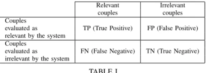
Precision is an evaluation criterion very appropriate to the framework of an unsupervised approach. Precision calculates the proportion of relevant couples of elements extracted among extracted couples. Using the notations of table I, the precision is given by the formula (15).

P recision = T P

(8)

A 100% precision means that all the couples extracted by the system are relevant.

Another typical measurement of the machine learning ap-proach is recall which computes the proportion of relevant couples of elements extracted among relevant couples. The recall is given by the formula (16).

Recall = T P

T P + F N (16)

A 100% recall means that all relevant couples of elements have been found. This measurement is adapted to the supervised machine learning methods where all positive examples (relevant couples of elements) are known.

Relevant Irrelevant couples couples Couples

evaluated as TP (True Positive) FP (False Positive) relevant by the system

Couples

evaluated as FN (False Negative) TN (True Negative) irrelevant by the system

TABLE I

CONTINGENCY TABLE AT THE BASE OF EVALUATION MEASUREMENTS.

It is often important to determine a compromise between recall and precision. We can use a measurement taking into account these two evaluation criteria by calculating the F-measure [16] :

F − measure(β) = (β

2

+ 1) × P recision × Recall

(β2_{× P recision) + Recall} (17)

The parameter β of the formula (17) regulates the respective influence of precision and recall. It is often fixed at 1 to give the same weight to these two evaluation measurements.

B. Evaluation protocol

To evaluate the results of our work, we need an oracle that we can trust. We choose the domain expert as an oracle. Although it may be considered as a tiresome task because of the manual checking, dictionnaries like Wordnet [17] would not have been efficient. Indeed the schemas contains some acronyms or terms that need to be tokenized.

The aim of this evaluation is to show that Approxivect finds higher similarity measures for similar elements. So the idea is to sort all discovered similarities and to check if the similar elements are in the top of this ranking. We then calculate the precision, recall and F-measure on the top-third of the ranking. The schemas used in the following experiments are Figure 1 and Figure 2. When matching the two schemas, an expert

should discover 9 relevant possibilities. Approxivect returns a ranking of 39 similarities, sorted by descending similarity measure. An extract of this ranking4 is shown in table II. In the relevance column, a + denotes a true positive (TP) whereas an empty cell stands for a false positive (FP). Note that when two couples with the same similarity are discovered, Approxivect ranks them in a random order.

Rank Element from Element from Similarity Relevance schema 1 schema 2 Measure

1 Professor Professor 1.0 + 2 CS Dept Australia People 0.46

3 Courses Grad Courses 0.41 + 4 CS Dept Australia CS Dept U.S. 0.36 + 5 Courses Undergrad Courses 0.28 + 6 Academic Staff Faculty 0.25 + 7 Staff People 0.23 + 8 Technical Staff Staff 0.21 + 9 Senior Lecturer Assistant Professor 0.16

10 Professor Assistant Professor 0.16

11 Senior Lecturer Associate Professor 0.16 + 12 Professor Associate Professor 0.16

13 Senior Lecturer Professor 0.16 ... ... ... ...

TABLE II

AN EXAMPLE OFAPPROXIVECT RANKING

Example : With the table II, we can calculate the measures explained in V-A. The precision is the number of discovered true positives on the number of both TP and FP. Actually the sum of TP and FP represents the number of extracted couples by Approxivect.

P recision = 8

8 + 5= 0.62 (18)

Then we can calculate the recall, which is the number of true positives on the number of both TP and FN. The sum of TP and FN can also be seen as the number of all relevant couples.

Recall = 8

8 + 1 = 0.89 (19)

Finally, we can obtain the F-measure which represents the compromise between precision and recall. We set the β parameter to 1.

F − measure = 2 × 0.62 × 0.89

0.62 + 0.89 = 0.73 (20)

Next we discuss each parameter, except for

SIM THRESHOLD, which is tuned to 0, because our aim is to rank the similarities. So we need them all. In the

4_{The parameters used for this example are :} _{NB LEVELS} _{= 1,} _RE

(9)

following tables, lev means Levenhstein distance and 3gram stands for tri-grams. Their aggregation is noted SM, and we selected two ways of aggregating those similarities: the maximum, noted max(lev, 3gram), and the average, noted

lev+3gram

2 . CM represents the cosine measure between the

context of two elements and it is aggregated with SM either by choosing the maximum, noted max(SM, CM), or by calculating the average SM +CM₂ . The given results only concerns the first third of the ranked similarities. This to show that Approxivect ranks the relevant similarities at the top of the ranking couples.

Discussion about NB LEVELS

Here we vary theNB LEVELSparameter to know if it is in-teresting to include in the context far ancestors or deep descen-dents. The other parameters are fixed : MIN WEIGHTis set to 1 so that we accept all the neighbours,REPLACE THRESHOLD

to 0.2 and K to 1.

Precision Recall F-measure

NB LEVELS= 1 max(lev, 3gram) 0.31 0.45 0.37

lev+3gram

2 0.62 0.89 0.73 NB LEVELS= 2 max(lev, 3gram) 0.46 0.67 0.55

lev+3gram

2 0.39 0.56 0.46

TABLE III

EXPERIMENTS ON NB LEVELS WITH MAX(SM , CM )

NB LEVELS= 1 max(lev, 3gram) 0.39 0.56 0.46

lev+3gram

2 0.31 0.45 0.37

TABLE IV

EXPERIMENTS ON NB LEVELS WITHSM +CM₂

The tables III and IV show that the number of levels should not be too high. Good results are obtained when it is set to 1, but they decrease with higher values. So the context should be limited to the first or second levels, to the nodes that are semantically closer. Note that this parameter could have been studied deeper : the number of levels up and down could have been different, so that either the ancestors or the descendants are prioritized.

Discussion about REPLACE THRESHOLD

Here we vary the REPLACE THRESHOLD parameter, which is the minimum threshold so that two terms are replaced. The adopted strategy between the terminological algorithms, namely the maximum or the average, is an important criteria since it is used to calculate the similarity that is compared

to this threshold parameter. The goal of this experiment is to demonstrate that replacing too many strings might involve bad results. Indeed there is no guarantee that the replacements are done on relevant similar couples. In the tables V and VI, the Repl column indicates the number of replacements. The other parameters are fixed :MIN WEIGHTis set to 1,NB LEVELSto 1 andKto 1. For the same reason as before,SIM THRESHOLD

is set to 0.

Repl Precision Recall F-measure

REPLACE max(lev, 3gram) 4 0.31 0.45 0.37 THRESHOLD = 0.2 lev+3gram₂ 2 0.62 0.89 0.73

REPLACE max(lev, 3gram) 1 0.54 0.78 0.64

THRESHOLD = 0.3 lev+3gram₂ 1 0.54 0.78 0.64

TABLE V

EXPERIMENTS ON REPLACE THRESHOLD WITH MAX(SM , CM )

On the first line of table V, the following 4 replacements occur :

• Professor ↔ Professor

• Courses ↔ Grad Courses

• Senior Lecturer ↔ Undergrad Courses

• Lecturer ↔ Courses

On these 4 replacements, 2 of them are false positives. Thus involving bad results when the context is then used to discover similarities. So it is better to avoid too many replacements.

Repl Precision Recall F-measure

TABLE VI

EXPERIMENTS ON REPLACE THRESHOLD WITHSM +CM₂

With a threshold above 0.3, precision and recall do not vary anymore. As the schemas used are quite small, there are not so many replacements occuring. Thus this parameter may need to be tested against larger schemas. Besides the Levenhstein distance and the 3-grams are maybe not sufficient enough to decide whether or not to replace terms. They focuse on the characters in the terms and could be completed by another algorithm that works on the tokens of a term.

Discussion about K

TheKparameter is used in the weight formula 9. Increasing

K implies to give more importance to the context. In this experiment, the other parameters are fixed : MIN WEIGHT is set to 1, NB LEVELS to 1, REPLACE THRESHOLD to 0.2 and

(10)

Precision Recall F-measure K= 1 max(lev, 3gram) 0.31 0.45 0.37 lev+3gram 2 0.62 0.89 0.73 K= 2 max(lev, 3gram) 0.23 0.34 0.27 lev+3gram 2 0.62 0.89 0.73 K= 4 max(lev, 3gram) 0.23 0.34 0.27 lev+3gram 2 0.62 0.89 0.73 TABLE VII

EXPERIMENTS ON K WITH MAX(SM , CM )

K= 1 max(lev, 3gram) 0.39 0.56 0.46 lev+3gram 2 0.54 0.78 0.64 K= 2 max(lev, 3gram) 0.31 0.45 0.37 lev+3gram 2 0.54 0.78 0.64 K= 4 max(lev, 3gram) 0.31 0.45 0.37 lev+3gram 2 0.62 0.89 0.73 TABLE VIII EXPERIMENTS ON K WITHSM +CM₂

Varying the K parameter is interesting. When using the maximum between the Levenhstein distance and the 3-grams, increasing K gives worse results. On the contrary, with the average between the two distances, increasing K enables to rank better the relevant couples. And the more we increaseK, the higher rank the relevant couples have. But with K above 4, results seem to be constant. So K depends on the adopted

strategy. But this experiment conforts the idea that the average between the terminological algorithms gives better results.

Discussion about MIN WEIGHT

Finally this last parameter is a constraint for the context and aims at showing the importance of the closest elements : if the weight of a node is not above theMIN WEIGHTthreshold, then it is not included in the context. The weight, given by the formula 9, is in the interval [1, K+1], and as we set K

to 1 for these experiments, the weight may vary between [1, 2]. With a MIN WEIGHT of 1, all neighbour nodes are

included in the context - if the other constraints are respected, namely NB LEVELS. Here we set NB LEVELS to 1, so the parent, children, siblings and cousins may be included in the context. By changingMIN WEIGHTto 1.25, this context is then restricted to the parent, children and siblings. And when set to 1.5, only the parent and children are included in the context. The other parameters are fixed : Kis set to 1,NB LEVELSto 1, REPLACE THRESHOLD to 0.2 and SIM THRESHOLDto 0.

So including the cousins in the context is not recommended. However we notice that those good results quickly decrease when the context is very limited, namely to the parent and children of a node. Indeed the similarity measure found in those cases quickly reaches values near 0 in the ranking table. Note that in table IX, we have a configuration that enables to find all the relevant similarities in the first third of the ranking.

MIN WEIGHT= 1 max(lev, 3gram) 0.31 0.45 0.37

lev+3gram

2 0.62 0.89 0.73 MIN WEIGHT= 1.25 max(lev, 3gram) 0.31 0.45 0.37

lev+3gram

2 0.69 1 0.82 MIN WEIGHT= 1.5 max(lev, 3gram) 0.39 0.56 0.46

lev+3gram

2 0.39 0.56 0.46

TABLE IX

EXPERIMENTS ON MIN WEIGHT WITH MAX(SM , CM )

MIN WEIGHT= 1 max(lev, 3gram) 0.39 0.56 0.46

lev+3gram

2 0.39 0.56 0.46

TABLE X

EXPERIMENTS ON MIN WEIGHT WITHSM +CM₂

General discussion

The main conclusion of these experiments is that the maximum between the cosine measure (CM) and the string mesure (SM) combined with the average between Levenhstein distance and 3-grams offer better results.

Approxivect has many parameters that need to be tuned. Although this may be seen as a drawback, it is quite obvious that some of them should not be too high. For example, Approxivect should limit the context nodes to the first or second level up and down in the hierarchy. And the context should include the descendants, ancestors and siblings, but should avoid the cousin nodes. According to the adopted strategy (maximum or average), the importance of the context may be increased a little. The threshold to replace terms must be tested with larger schemas. The parameter SIM THRESHOLD, which has not been tested here, might be used to only discover the similarities above a certain threshold. However using this parameter is probably not sufficient enough to discover mappings, or it must be completed by some algorithms to select the relevant couples in the ranking. Finally a machine learning system could be an interesting future work in order to tune automatically these parameters.

C. Comparison with COMA++

To our knowledge there is no tool that tries to rank the similarities between elements of two schemas. So to compare our work, we decided to use some matching tools. But the matchers do not offer the possibility to rank all the similarities they processed. Instead they display the mappings, namely the couples of elements they consider similar. So we apply COMA++ on the same schemas 1 and 2. All the COMA++ strategies have been tried and the best obtained results are

(11)

shown in the following table XI. All those discovered map-pings are relevant.

Element from Element from Similarity schema 1 schema 2 Measure

Courses Grad Courses 0.5041725 Courses Undergrad Courses 0.5041725 Professor Professor 0.53545463 Technical Staff Staff 0.5300107 CS Dept Australia CS Dept U.S. 0.52305263

TABLE XI

RESULTS OBTAINED WITHCOMA++ON SCHEMAS1AND2

COMA++ found 5 mappings on the 9 relevant similarities, implying that 4 mappings are never discovered. The recall is 0.56, the precision is obviously 1 since the extracted list gives only the relevant similarities. We obtain a F-measure equal to 0.72. Even if it is quite difficult to compare those figures, Approxivect has in the optimal configurations a F-measure equal or above to 0.73. Those configuration enables to discover between 7 and 9 relevant similarities, compared to the 5 given by COMA++.

Our aim is not to find mappings - our algorithm has not been designed for that since it does not include as many algorithms as matching tools5 _{- but the comparison with}

COMA++ might help to judge on the results of Approxivect.

VI. CONCLUSION

In this paper we have proposed an hybrid method, Approxivect, to measure the similarity between two elements of different schemas. Some interesting features include the language and domain independance, and the fact that it does not use any dictionnary or ontology. Indeed Approxivect is based on the notion of context of a schema node and on different terminological measures. The context of a given node includes some of its neighbours according to the value of Approxivect parameters and the weight formula. The Levenhstein distance and 3-grams are commonly used to compare character strings, and are well suited in our method. They are completed by the cosine measure, which evaluates the similarity between two sets of terms. The combination of those measures enables to find similarities between couples of elements, the terminological measures ensuring to detect the terms whose terminologies are close while the context allows to discover similarities between the other terms. The experiments section showed that Approxivect gives good results. By ranking all similarities found by our approach, we notice that most of the relevant couples were ranked in the beginning of the ranking. By comparing the results with COMA++, it appears that Approxivect, when its parameters are tuned in optimum configurations, discovers most of the relevant couples in the top ranking while COMA++ only finds half of the mappings. The experiments

5_{However it could be enhanced to reach this goal}

also enabled to fix some parameters, and some of them could be improved by deeper tests.

This work is essentially a first step, and it involves many perspectives in different domain applications. The first one would be to use other algorithms to compare terms, like the one presented in the related work section. Another future work concerns the schema matching : Approxivect could be enhanced with more algorithms to extract mappings from the ranking. And in a large scale schema matching scenario, with a dynamic environment, it may be a good idea to use the context. Instead of sending a whole schema or a random part of it on the network, determining a subtree that includes the important context nodes seems to be a good idea to spare resources [18]. This approach consisting in processing the semantic proximity between schema elements may also be an important task when building automatically ontologies [19] or to align them [12], [20]. Finally machine learning techniques could bring more flexibility by tuning automatically the parameters. Even if our experiments showed a good configuration of the parameters, some specific domains might need softer or harder constraints. Thus machine learning would result in a process without the expert intervention.

REFERENCES

[1] D. Lin, “An information-theoretic definition of similarity,” in Proc. 15th International Conf. on Machine Learning. Morgan Kaufmann, San Francisco, CA, 1998, pp. 296–304. [Online]. Available: citeseer.ist.psu.edu/95071.html

[2] A. Doan, J. Madhavan, P. Domingos, and A. Halevy, “Ontology matching: A machine learning approach,” in Handbook on Ontologies, International Handbooks on Information Systems, 2004.

[3] E. Rahm and P. A. Bernstein, “A survey of approaches to automatic schema matching,” VLDB Journal: Very Large Data Bases, vol. 10, no. 4, pp. 334–350, ???? 2001. [Online]. Available: citeseer.ist.psu.edu/rahm01survey.html

[4] M. Yatskevich, “Preliminary evaluation of schema matching systems,” University of Trento, Tech. Rep. DIT-03-028, Informatica e Telecomu-nicazioni, 2003.

[5] J. Tranier, R. Barar, Z. Bellahs`ene, and M. Teisseire, “Where’s charlie: Family-based heuristics for peer-to-peer schema integration,” in Proc of IDEAS, 2004, pp. 227–235.

[6] A. Maedche and S. Staab, “Measuring similarity between ontologies,” in Proc. of the European Conference on Knowledge Acquisition and Management - EKAW, 2002, pp. 251–263. [Online]. Available: citeseer.ist.psu.edu/maedche02measuring.html

[7] D. Aumueller, H. Do, S. Massmann, and E. Rahm, “Schema and ontology matching with coma++,” in SIGMOD 2005, 2005.

[8] S. Melnik, H. G. Molina, and E. Rahm, “Similarity flooding: A versatile graph matching algorithm and its application to schema matching,” in Proc. of the International Conference on Data Engineering (ICDE’02), 2002.

[9] J. Euzenat et al., “State of the art on ontology matching,” Knowledge Web, Tech. Rep. KWEB/2004/D2.2.3/v1.2, 2004.

[10] W. Cohen, P. Ravikumar, and S. Fienberg, “A comparison of string distance metrics for name-matching tasks,” in In Proceedings of the IJCAI-2003., 2003. [Online]. Available: citeseer.ist.psu.edu/cohen03comparison.html

[11] W. Winkler, “The state of record linkage and current research problems,” in Statistics of Income Division, Internal Revenue Service Publication R99/04, 1999.

[12] H. Kefi, “Ontologies et aide à l’utilisateur pour l’interrogation de sources multiples et hétérogènes,” Ph.D. dissertation, Université de Paris 11, 2006.

[13] J. Madhavan, P. Bernstein, and E. Rahm, “Generic schema matching with cupid,” in VLDB01, 2001.

(12)

[14] R. Wilkinson and P. Hingston, “Using the cosine measure in a neural network for document retrieval,” in Proc of ACM SIGIR Conference, 1991, pp. 202–210.

[15] M. Sayyadian et al., “Tuning schema matching software using synthetic scenarios,” in Proceedings of the 31th VLDB Conference, 2005. [16] C. Van-Risbergen, Information Retrieval. 2nd edition, London,

Butter-worths, 1979.

[17] G. Miller, R. Beckwith, C. Fellbaum, D. Gross, and K. Miller., “Intro-duction to WordNet: an on-line lexical database,” International Journal of Lexicography, vol. 3, no. 4, pp. 235–244, 1990.

[18] P. Bouquet, L. Serafini, and S. Zanobini, “Peer-to-peer semantic coordination,” Journal of Web Semantics, vol. 2, no. 1, pp. 81–97, 2004. [Online]. Available: http://www.websemanticsjournal.org/ps/pub/2005-6 [19] N. Aussenac-Gilles and D. Bourigault, “Construction d’ontologies `a

partir de textes,” in Actes de TALN03, vol. 2, 2003, pp. 27–47. [20] A. Doan, J. Madhavan, P. Domingos, and A. Halvey, “Learning to map