Human Capital Investment by the Poor: Informing Policy with Laboratory and Field Experiments

Texte intégral

(1)2010s-33. Human Capital Investment by the Poor: Informing Policy with Laboratory and Field Experiments Catherine Eckel, Cathleen Johnson, Claude Montmarquette. Série Scientifique Scientific Series. Montréal Août 2010. © 2010 Catherine Eckel, Cathleen Johnson, Claude Montmarquette. Tous droits réservés. All rights reserved. Reproduction partielle permise avec citation du document source, incluant la notice ©. Short sections may be quoted without explicit permission, if full credit, including © notice, is given to the source..

(2) CIRANO Le CIRANO est un organisme sans but lucratif constitué en vertu de la Loi des compagnies du Québec. Le financement de son infrastructure et de ses activités de recherche provient des cotisations de ses organisations-membres, d’une subvention d’infrastructure du Ministère du Développement économique et régional et de la Recherche, de même que des subventions et mandats obtenus par ses équipes de recherche. CIRANO is a private non-profit organization incorporated under the Québec Companies Act. Its infrastructure and research activities are funded through fees paid by member organizations, an infrastructure grant from the Ministère du Développement économique et régional et de la Recherche, and grants and research mandates obtained by its research teams. Les partenaires du CIRANO Partenaire majeur Ministère du Développement économique, de l’Innovation et de l’Exportation Partenaires corporatifs Banque de développement du Canada Banque du Canada Banque Laurentienne du Canada Banque Nationale du Canada Banque Royale du Canada Banque Scotia Bell Canada BMO Groupe financier Caisse de dépôt et placement du Québec Fédération des caisses Desjardins du Québec Gaz Métro Hydro-Québec Industrie Canada Investissements PSP Ministère des Finances du Québec Power Corporation du Canada Raymond Chabot Grant Thornton Rio Tinto State Street Global Advisors Transat A.T. Ville de Montréal Partenaires universitaires École Polytechnique de Montréal HEC Montréal McGill University Université Concordia Université de Montréal Université de Sherbrooke Université du Québec Université du Québec à Montréal Université Laval Le CIRANO collabore avec de nombreux centres et chaires de recherche universitaires dont on peut consulter la liste sur son site web. Les cahiers de la série scientifique (CS) visent à rendre accessibles des résultats de recherche effectuée au CIRANO afin de susciter échanges et commentaires. Ces cahiers sont écrits dans le style des publications scientifiques. Les idées et les opinions émises sont sous l’unique responsabilité des auteurs et ne représentent pas nécessairement les positions du CIRANO ou de ses partenaires. This paper presents research carried out at CIRANO and aims at encouraging discussion and comment. The observations and viewpoints expressed are the sole responsibility of the authors. They do not necessarily represent positions of CIRANO or its partners.. ISSN 1198-8177. Partenaire financier.

(3) Human Capital Investment by the Poor: Informing Policy with Laboratory and Field Experiments* Catherine Eckel†, Cathleen Johnson ‡, Claude Montmarquette§. Résumé Le but de cette étude est de recueillir des informations pour concevoir une politique publique afin d’inciter les pauvres à investir en capital humain. Nous utilisons l’approche expérimentale pour mesurer les préférences et les choix de la population ciblée. Nous avons recruté 256 sujets à Montréal. 72 % avaient un revenu inférieur à 120 % pour cent du seuil de faible revenu de Statistique Canada. La combinaison de mesures d'enquête et les décisions réelles nous permettent de mieux comprendre l'hétérogénéité individuelle dans les réponses aux différents niveaux de subvention. Deux caractéristiques comportementales, la patience (désir d’épargne) et l'attitude envers le risque, sont essentielles à la compréhension des déterminants de l'investissement éducatif pour les personnes à faible revenu dans cette expérience. La décision d’investir dans l'éducation d'un membre de la famille est quelque peu différente de celle d'investir dans sa propre éducation. Encore une fois, les participants les plus patients sont les plus susceptibles d'épargner pour l'éducation d'un membre de la famille, mais au contraire, investir dans sa propre éducation, l'attitude d'un sujet vis-à-vis le risque ne joue aucun rôle. Mots clés : choix intertemporels, expériences sur le terrain, les attitudes visà-vis le risque, travailleurs pauvres. *. We thank Kate Krause, Scott Murray, Arthur Sweetman, Glenn Harrison, Jeff Carpenter, and participants at various seminars for their helpful comments and suggestions. Special thanks to Nathalie Viennot-Briot for her programming expertise and Jean-François Houde for his assistance in conducting the experimental sessions. We are indebted to Jean-Pierre Voyer for securing the funding for this research and for his commitment to investigating policy through experimentation. This work was funded under a contract through the Social Research and Demonstration Corporation from Human Resources Development Canada, Applied Research Branch. Any remaining errors are the sole responsibility of the authors. † School of Economics, Political and Policy Sciences, University of Texas at Dallas, eckelc@utdallas.edu. ‡ Affiliation University of Arizona and CIRANO, cathleen@email.arizona.edu. § CIRANO and University of Montreal, montmarc@cirano.qc.ca..

(4) Abstract The purpose of the study is to collect information that can be used to design a policy to induce the poor to invest in human capital. We use laboratory experimental methodology to measure the preferences and choices of the target population of a proposed government policy. We recruited 256 subjects in Montreal, Canada; 72 percent had income below 120 percent of the Canadian poverty level. The combination of survey measures and actual decisions allows us to better understand individual heterogeneity in responses to different subsidy levels. Two behavioral characteristics, patience and attitude towards risk, are key to understanding the determinants of educational investment for the low-income individuals in this experiment. The decision to save for a family member’s education is somewhat different from that of investing in one’s own education. Again, patient participants were more likely to save for a family member’s education, but in contrast to investing in one’s own education, a subject’s attitude towards risk played no role. Keywords: Intertemporal choice, field experiments, risk attitudes, working poor Codes JEL : C93, D91, D81.

(5) I.. Introduction. Returns to investment in human capital have been high in the last half of the 20th century, but at the bottom of the income distribution, the decision to invest in education beyond high school is still seen as complex and risky (Chen, 2002). To the educated, investment in education seems the obvious and only way to escape poverty, yet the poor avoid such investments. We report the results of a study designed to understand why the poor fail to invest in human capital. The purpose of the study is to collect information that can be used to design a policy to induce the poor to save and invest in human capital. We use laboratory experimental methodology to measure the preferences and choices of the target population of a proposed government policy. Note that our purpose is not to evaluate such a policy; in particular, we do not attempt to discover the return to additional human capital investment. Instead, we focus on preferences for education, and assess the response of the choices of the poor population to various subsidy levels. Laboratory experimentation as a research tool is widely applied to study the design of institutions, to test the implications of game theory, and to examine individual decision-making. In contrast, our approach is to use experiments as tools in the field to measure the underlying preferences of the poor, and to examine their actual choices to invest in human capital in a field experiment. Experimental research provides a potentially fruitful approach to collecting information in order to design, calibrate, and estimate the impact and cost of specific government policies.1 Our study is notable in several respects. First, our subjects are the target population for the proposed policy intervention: the adult working poor in Canada. We recruited 256 subjects in Montreal, Canada; 72 percent had income below 120 percent of the Canadian poverty level.2 Thus we examine the response of subjects who represent the population of interest, and gauge their responsiveness to a range of policy parameters. Second, the study combines attitudinal survey questions with incentivized choices -- experiments – involving real choices between 1. Roth (2002) makes the case for the use of experimental research in the design of market and nonmarket institutions. His discussion focuses on the use of experiments to estimate the response of markets and other institutions to changes in structure and parameters. Our study focuses on the direct measurement of preferences. 2 Statistics Canada annually publishes a set of measures called the low income cut-offs (LICOs). Roughly speaking, the cut-offs mark income levels in which people have to spend disproportionate amounts of their income on food, shelter, and clothing. The LICOs vary by family size and size of community. Before-tax income cut-offs were used in view of the fact that before-tax income data was collected from the respondents. 1.

(6) amounts of money and policy-relevant alternatives to assess policy impact. The experiments are of two types: one type involves decisions that are designed to measure the subjects’ risk attitudes and time preferences; the second type consists of decisions trading designed to measure willingness to invest in education for themselves or for family members. In this second set of choices, subjects choose between cash amounts and higher amounts that are earmarked for educational investment. The combination of survey measures and actual decisions allows us to better understand individual heterogeneity in responses to different subsidy levels. A third innovation is that the experiments, especially those involving actual human capital decisions, involve high stakes. Subjects make 63 decisions, with $25-$600 CA at stake: at the end of the experiment, one decision is chosen randomly for payment.. Average earnings were $147. including a $12 show-up fee. Our study provides high-stakes measures of risk, time preference, and savings choices. In particular the incentives are high enough that subjects could increase human capital investment by taking one or more courses at a Montreal technical, career, trade or community college.3 Our data permit an unusually rich analysis of the decision to invest in human capital. Controlling for demographic characteristics such as age, sex, family structure and income, we can examine the role of risk attitudes and time preference in the investment decision. We also can test for the responsiveness of various subsets of the poor population to subsidies targeted toward their own education as well as that of their children. In section II, we discuss the human capital decision of the adult poor. In section III, we present our research design and methods. The experimental results are discussed in section IV. A concluding section ends the paper.. II.. The Human Capital Decision of Adults When considering an investment in education, it is well known that an individual will. consider opportunity cost along with evaluating the potential benefit. Traditional research has focused mainly on the decision to enter the labor market or to continue formal training. Risk attitudes and a preference for current consumption over future consumption are recognized as important factors contributing to the schooling decision (Weiss, 1972). The importance of credit. 3. See www.canadian-universities.net for a listing of such schools. At the time of the study, single courses cost $30$300. 2.

(7) constraints for some groups was also investigated, but remains an unsettled issue (Dynarski, 2002). Aversion to debt among low-income individuals may also play a role (Eckel et al. 2007). The context of the investment decision may differ considerably, depending on the age of the decision maker. Adults may see the choice very differently from high-school age decision makers. Some adults might have experienced personal failures such as marital difficulties, unstable working conditions with recurrent spells of unemployment, or prior low-returning educational investments. Furthermore, adults with children face additional time and financial constraints. Thus, for adults, the decision to undertake an educational program appears more complex and more risky than for younger decision makers. For poor adults, all of the considerations listed above will be compounded with financial constraints. This suggests that the barriers to a decision to accept and invest in educational opportunities for the adult poor are numerous and important. Consideration of the role of individual attitudes towards risk and consumption over time in the education decision are not new in the human capital literature. Levahari and Weiss (1974) produced an early study on the role of risk and uncertainty on investment in human capital using a Fisherian two-period model. They show that uncertainty is an important factor, but that the effect of increased uncertainty is ambiguous and is content and context-dependent. For Chen (2002), reluctance to attend college by some young people is explained by the risks of investment in education that result from incomplete information about individual ability, the quality of education and unanticipated modifications in labor market conditions. Chen suggests that when discussing investment in human capital, it is important to distinguish attitudes toward risk from perceptions of risk. A risk-averse high school student might prefer education to the labor market if she perceives the risk in the labor market to be greater than continuing with her schooling. For this person, the labor market is not only risky, but also uncertain because of her lack of experience in that sector of activity. For a labor market participant, the situation is essentially reversed: an investment in human capital appears more risky or uncertain than what she might have experienced in the labor market. Therefore, with the same risk-averse attitude, a person of school age will prefer to continue with her investment in education, while an adult will prefer to remain in the labor market. Time preference is also a key factor in the decision to invest in human capital. The decision to forego current for future consumption is fundamental for human capital theory, which. 3.

(8) relies heavily on the discounted utility model first proposed by Samuelson (1937).4 Human capital investment features early costs and returns late in the life cycle. In the standard decision framework with perfect credit markets, individuals maximize the present value of lifetime income using market interest rate to discount future earnings and allocate consumption over time according to their own rate of time preference (see Heckman, Lochner and Todd, 2008 for a thorough discussion on the earning function and rates of return). Our experiment also may inform the debate on the importance of liquidity constraints in human capital decisions by adults. In a study of the Pell Grant education-funding program, Stefor and Turner (2002) show that changes in the availability of US Federal aid have a significant effect on the schooling enrollment of adults. Bound and Turner (2002) find that the net effects of funding through the G.I. Bill led to substantial gains in the post-secondary educational attainment of World War II veterans, comparable to recent estimates of enrollment responses to changes in tuition rates. Our study also examines willingness to make investments in human capital for a family member. In the experiment the identity of the family member is not restricted, but in practice subjects typically considered the education of a child in their household. For this decision, the effect of a decision-maker’s own risk and time preferences are likely to be less relevant. The risk of failure then applies to others, and patience or future orientation may also be less critical when decisions are made for children or other family members.. Furthermore, in this situation. borrowing constraints might become the most important issue for poor families, even when parents are fully cognizant of the importance of investing in the human capital of their children. Empirical evidence that the rate of return for education is higher for low-income youth is consistent with binding liquidity or borrowing constraints. (See Keane (2002) for a discussion of the limitations of this evidence.) However, studies by Cameron and Heckman (1998), Keane and Wolpin (2001), and Keane (2002) produce structural estimates to suggest that borrowing constraints have had little effect on college attendance decisions. Human-capital accumulation prior to college age is seen as playing a much more important role. Thus, if schooling decisions. 4. This model assumes that a person’s preferences are time-consistent: that he will make the same choice no matter when he or she is asked. In a review of empirical and experimental studies of discount rates, Frederick, Loewenstein and O’Donoghue (2002) note evidence that discount rates are not constant. They conclude that discount rates may decline over time, gains are discounted more than losses, and small amounts more than large amounts. The impact of these issues has not been worked out in the context of human capital investment decisions. 4.

(9) come earlier in the family life cycle, these authors consider that government policies might have a major impact on the children of poor families.. III.. Research Design and Methods This section describes the design and operational details of the laboratory experiment. To. maximize the policy relevance of the results, we recruited subjects from the population that the policy is designed to target. Recruitment efforts were organized through YMCA and work recruitment centers, whose membership included many working poor. To advertise and recruit for the experiment, a brief notice was posted in low-income neighborhoods and distributed at community group meetings. No information about the purpose of the study was revealed; potential subjects were told only that they would be paid a $12 show-up fee, and would have the opportunity to earn more in the course of the 90-minute study. Subjects volunteered for the experiment by calling ahead and agreeing to show up at a time and location identified by the experimenters. All of the experimental sessions were held in Montreal over a period of three weeks in November 2000. A total of 256 subjects participated; summary sample statistics are shown in Table 1, with comparisons to population groups. Sixty-three percent had family income less than the Statistics Canada low-income cut-off (LICOs) for their family size and composition.5 Average total family income for the entire sample was approximately $22,500 CAD. Seventy-two percent of the subjects were labor market participants, either employed or unemployed. Two thirds of the subjects were women. Participants were far from uneducated: on average, they reported completing 13 to 14 years of schooling: 78 percent held a high-school diploma, and 26 percent reported completing a university degree.6 Nor were the subjects without assets or access to capital markets: 26 percent owned a car, and 54 percent possessed a credit card. A significant fraction planned for the future: 47 percent declared that they made regular contributions to a savings account, and 27 percent contributed to a retirement plan. 5. The LICOs vary based on family size and location. In 2000, for a family of four in an urban setting, the before-tax LICO was 24,565 (See Statistics Canada 2001 for details). 6 Some participants who had not been targeted by the recruitment efforts were still able to learn about the experiment. Word of mouth about the experience and the potential for substantial sums of cash traveled fast, even in a relatively large city like Montreal. The largest group of unintended recruits was full-time students; the 31 students represent 12 percent of the total number of subjects. Care was taken to identify this subgroup separately in the analysis. 5.

(10) Table 1: Sample and Population Characteristics, N=256 Population Mean 34.7a 0.447b 1.102b,c. Sample Mean 33.71 0.332 0.633. Std.Dev.. Minimum. Maximum. 10.43 0.472 0.953. 17 0 0. 70 1 4. Non-Labor Force* Student. n/a 0.182a. 0.121 0.121. 0.327 0.327. 0 0. 1 1. Schooling (years) High School Diploma University degree. n/a 0.796a 0.308c. 13.60 0.781 0.258. 2.81 0.414 0.438. 3 0 0. 16 1 1. Low Income (below 100% LICO). 0.231. 0.629. 0.449. 0. 1. Age Male Number of Children. *Main activity is housework or taking care of family n/a: not available a Population of the city of Montreal. b Poor population in Montreal. c Authors’ estimate based on census data.. 3.1 Procedure Once all participants were assembled, subjects were given a $12 show-up fee, and the potential for additional financial compensation was explained and demonstrated.. Subjects. completed the two components of the study, each of which was contained in a booklet for ease of administration and record keeping. One booklet contained 64 experimental decisions, and the other contained 43 questions collecting demographic and household information. Every effort was made to make the experiment accessible and non-threatening to all of the subjects. No computers were used, and simple devices like bingo balls and dice were used to generate random draws. Special attention was paid to the visual presentation and design of the experimental decisions. To ensure comprehension, a short set of practice decisions was incorporated into the instruction portion of the session. An example of each type of decision and the random draw process used to determine payment was illustrated in a six-decision practice. Instructions for the experiment are detailed in Appendix A. In the debriefing questionnaire, 95 percent of the subjects indicated that they were confident they would be paid in the way that was described to them in the experiment.. 6.

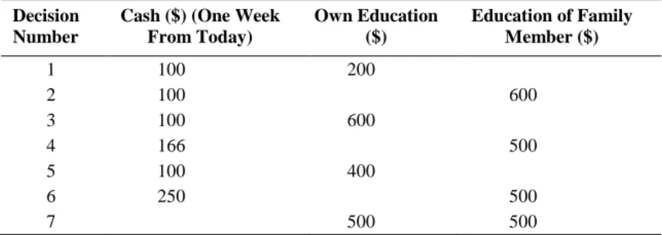
(11) At the end of the experiment one of the 64 experimental decisions was selected for payment using a bingo cage containing 64 balls, numbered 1 to 64. The number on the ball drawn from the cage identified the experimental decision for which they would be paid. If the decision involved a monetary prize on the same day of the experiment, the prize was given in cash, on site. Delayed payments for the time-preference task were mailed in the form of a postdated check for the date indicated in the experimental decision (2-28 days from the experiment). There were other forms of remuneration for the investment decisions, such as reimbursable educational expenses for own education and guaranteed investment certificates (GICs) for education for a family member. (A description of all forms of remuneration can be found in Appendix A.) When the prize was a GIC, the experimenter signed an IOU and the prize was delivered to the subject by courier approximately one month after the experiment. All participants were required to sign a receipt. The average payoff per participant resulting from the experiment was approximately $137 in addition to a $12 show up fee. Each experimental session, from instruction to payoff, took about an hour and a half.. 3.2 Experimental Decisions The experimental decisions were designed to address three main questions: (1) Will the working poor invest in human capital? (2) Are these subjects willing to delay consumption for substantial returns? (3) How do these subjects view risky choices? Thus three sets of experimental decisions were used to investigate these questions: (1) investment preferences, (2) time preferences, and (3) risk preferences. 3.2.a. Investment decisions.. Two sets of decisions involving human capital were. available to the participants: Investment in their own human capital or investment in a family member’s human capital. Table 2 summarizes the human capital investment preference decisions. Each row of the table represents the alternatives presented to the subject. Three decisions involve tradeoffs between cash and amounts earmarked for own education; three involve similar tradeoffs for a family member’s education. A final decision compares the two.7. 7. Note the full survey included decisions about retirement and durable goods investment that are not analyzed here. See Eckel, et al. (2005), for an analysis of the retirement decisions. 7.

(12) Table 2: Summary Description of Investment Decisions Decision Number 1 2 3 4 5 6 7. Cash ($) (One Week From Today). Own Education ($). 100 100 100 166 100 250. Education of Family Member ($). 200 600 600 500 400 500 500. 500. Figure 1 illustrates the way in which choices were presented to the subjects using one experimental decision. There were three versions of this decision, with $200, $400, and $600 for investment in education weighted against an offer of $100 cash (one week from the day the experimental session was conducted).. Figure 1: Sample Investment Decision You must choose A or B:.  . Choice A: $100 one week from today Choice B: $400 in your own training or education. These two choices are represented by the two following pictures. Please circle your choice: $400 in your own training or education $100 one week from today (expenses refunded) O or. Choice A. Choice B. The investment decisions were designed to test the subjects’ willingness to give up a $100 (one week from today) for reimbursable expenses for own education in the near term. For a family member’s education, a different procedure was used. Five-year, fixed, non-transferable Guaranteed Income Certificates (GICs) issued in the name of a family member were offered to 8.

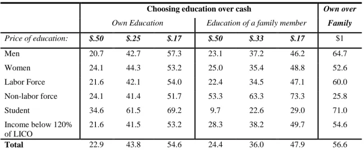
(13) subjects as a mechanism for such an investment. The lowest initial purchase of these GICs available at the time of the experiment was $500. Therefore to produce match rates similar to those for the own-education decisions and keep the participant payoffs within the limited budget of the experiment, the size of the cash alternative was varied. The match rates were chosen to help pinpoint optimal match rates for the policy design. While it would more closely mimic the proposed policy to have subjects save their own funds in exchange for an amount earmarked for investment in their education, that requirement would have made the administrative cost and timing of the laboratory experiment infeasible. The laboratory alternative to having subjects save their own funds was to give subjects the choice between $100 in cash provided by the experimenter and a specified amount in investment. In this context, in order to select the educational outcome, subjects would have to give up $100 in cash. Given the range of the subjects’ incomes, $100 represented a substantial amount of money to them. Aggregate results for the investment decisions are shown in Table 3. The first section in Table 3 indicates the percentage of subjects who chose $200, $400, or $600 earmarked for their own educational expenses over $100 cash one week from the date of the experiment. These choices represent match rates for education of 1, 3 and 5 to 1. At the lowest matching rate of 1 to 1, the price of education is $0.50, and just over a fifth (22.9 percent) of the participants chose education over cash. When subjects faced a 3/1 subsidy, the price of education is $0.25, and 43.8 percent of subjects chose education. Even at the highest matching rate of 5 to 1, that is a price of $0.1667, only 54.6 percent of participants chose own educational expenses.8 The take-up rate for savings for a family member’s education was a similarly modest 47.9 percent. Except for the Student subgroup, in which the rates of choosing education are, not surprisingly, consistently higher for all match rates, the patterns of behavior observed in other population subgroups are similar to the overall population. Comparing women and men, men appear to be more sensitive to the matching rate than the women, starting off with a lower percentage of take-up for the 1 to 1 match rate (20.7 percent vs. 24.1 percent) and ending with a 8. Because this choice entails giving up money they would otherwise receive from participating in the experiment — i.e. ―house money‖ — rather than their own earned income, these results most likely overstate slightly the willingness of participants to forego current income for investment in human capital under the learn$ave program. If participants had to use their own funds and give up planned consumption to do so, one would expect the take-up rate to be lower. Note that the tradeoff ratios differ between own and family member because of constraints on the available financial instrument, in addition to a small calculation error in the design parameters. 9.

(14) higher take-up rate for the 5 to 1 match rate (57.3 percent vs. 53.2 percent). Low-income subjects, shown here as those with incomes less that 120 percent of the relevant LICO, do not differ significantly from the overall response levels (72 percent of the sample fell into this category).. Table 3: Percent Choosing Education. Choosing education over cash Own Education. Own over. Education of a family member. Family. Price of education:. $.50. $.25. $.17. $.50. $.33. $.17. $1. Men. 20.7. 42.7. 57.3. 23.1. 37.2. 46.2. 64.7. Women. 24.1. 44.3. 53.2. 25.0. 35.4. 48.8. 52.6. Labor Force. 21.6. 42.1. 54.0. 22.4. 34.5. 47.1. 60.0. Non-labor force. 24.1. 41.4. 51.7. 53.3. 63.3. 73.3. 25.8. Student. 34.6. 61.5. 69.2. 9.7. 22.6. 29.0. 71.0. Income below 120% of LICO Total. 21.6. 41.5. 53.2. 28.3. 38.2. 49.7. 54.6. 22.9. 43.8. 54.6. 24.4. 36.0. 47.9. 56.6. The second section of Table 3 represents the percentage of subjects who chose amounts earmarked for educational expenses of a family member over variable cash amounts one week from the date of the experiment. Here the matching rates are 1, 2, and 5 to 1. In the lowest subsidy rate offered, participants were asked to choose between $250 cash a week from the day of the experiment and a GIC with a $500 deposit value bearing interest with a fixed maturity of five years. If this certificate of deposit was won, the winning participant had to identify the bearer (family member recipient) on the day of the experiment. It was emphasized by the experimenter that those certificates were to be used for the education of a family member. Overall, when the price of education is $0.50, 24.4 percent of all participants chose the family member’s education over cash; at a lower price of $0.33, 36.0 percent chose the family member education, and at the lowest price of $0.1667, 47.9 percent chose family member education. Similar results hold for the Low Income subpopulation. However, for the participants declaring their main activity to be taking care of their family, these proportions are substantially higher at 53.3 percent, 63.3 percent, and 73.3 percent, respectively. This observation requires a deeper 10.

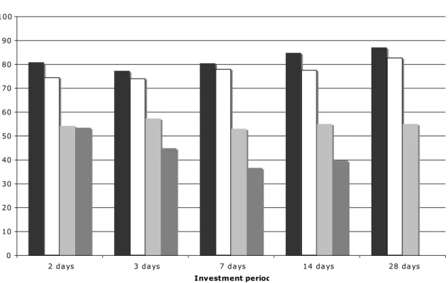
(15) look. A substantially smaller proportion of the Non-labor Force subpopulation chose education for themselves when faced with the same match rates (24.1 percent, 41.4 percent, and 51.7 percent respectively). In the last column of Table 3, proportions are summarized for the choice between $500 for their own education and $500 for a family member’s education. Here, the nonlabor force participants overwhelmingly choose their payoff in the form of family member’s education. All other subgroups choose their own education more often. It may be that members of this subpopulation consider an investment in education to be a better investment for family members than for themselves. Further analysis of family member education is undertaken below. 3.2.b. Time preference decisions. Time preferences were elicited by giving subjects a series of choices between a smaller sooner payment (SS) and a larger amount later (LL). If the subject chose the delayed payoff LL, the subject was rewarded for waiting. 37 decisions were constructed, varying the timing of the sooner payment (front end delay, FED = 0, 1, 7 or 14 days), the investment period (2-28 days), and the rate of return (10%, 50%, 200%, or 300%). Simple interest rates were used for simplicity, given the low education level of the subject pool. The longest time period was not included in the set of decisions with a 380% return for budgetary reasons. The SS were approximately $72, with one set of decisions at a lower SS of approximately $26. The decisions were presented to the subjects in random order. The full set of decisions is presented in Appendix B Table B.1. The proportion of impatient decisions for each is presented in Appendix C, Table C.3. These responses can be used to measure the overall degree of patience.9 Subjects were, overall, quite impatient. Five percent of participants (13 subjects) exhibited the most patient behavior by always choosing the later payment, while fifteen percent of the participants (43 subjects) chose the earliest payoff regardless of payoff, discount rates, or time delays. Figure 2 shows the distribution of decisions by rate of return and investment period. Overall the fraction choosing the earlier decision falls with the rate of return, as expected. For the 10% and 50% rates of return, impatient behavior increases slightly with the investment period; for 200% it says roughly constant over time; for 380% there is a slight decrease in impatient behavior with longer investment periods. 9. Since this experiment was conducted in November, 2000, alternative time-preference elicitation methods have been developed and used by other researchers, including Harrison, et al., 2002; Anderson et al., 2006; Burks et al., 2008. The task used here was developed by the authors, and was among the first attempts to elicit time preference in the lab. In subsequent studies, we and others have found that more consistent choices are made when decisions are presented to subjects in a coherent structure, rather than our approach, which produces substantial inconsistency. 11.

(16) Figure 2: Distribution of Impatient Choices FED = 7 for 10%, 50%, 200%, FED = 1 for 380% 100 90 80. % Choosing SS. 70 60 50 40 30 20 10 0 2 da ys. 3 da ys. 7 da ys. 14 da ys. 28 da ys. Investment period 10%. 50%. 200%. 380%. In short, 20 percent of the subjects were not affected by the parameters of the experiment: a 380 percent rate of return was not enough to induce 15 percent of the sample to save, and a 10 percent rate of return was not too low to discourage 5 percent of the sample to save, even for two days. On the other hand, at least eighty percent of the subjects were affected by the parameters of the experiment. Table 4 contains the results of a linear regression that shows the effect of the rate of return, investment period and absolute return on the decision to choose the sooner payment. It also includes a variable ―today‖ that is an indicator variable equal to 1 if the sooner payment was the day of the experiment (FED = 0). Controlling for other factors, the longer the subject had to wait between the earlier and later payoff dates, the more chose the earlier date. A higher rate of return as well as a higher absolute dollar return induced more subjects to wait for the higher, later amount. Finally, the ―today‖ variable carries an insignificant sign, which indicates that subjects were not more likely to take a payoff in hand on the day of the experiment. This is encouraging, as it indirectly implies that skepticism about whether future payoffs would be paid was not a factor in the 12.

(17) present-orientation of the decisions: subjects trusted the experimenters to pay the promised amounts on the promised dates. Table 4: Factors Affecting the Percentage of Participants Choosing the Earliest Payoff Choices for Each Time Preference Decision (Logistic Specification) Variable Constant Investment Perioda Todayb Absolute Returnc Rate of Returnd. Coefficient 0.968 *** 0.0414 *** 0.139 -0.137 *** -0.002 ***. t-statistic 8.06 4.69 0.85 -6.09 -4.80. R 2 = 0.817; 37 observations (1 for each decision) Bolded values and *** indicate coefficients statistically significant on the 0.1 percent level. a Investment Period is the number of days between the early payoff and later payoff. b Today is 1 if payoff is the day of the survey; 0 otherwise. c Absolute Return is the absolute difference between payoffs (Later Payoff - Early Payoff). d Rate of Return is the annualized rate of return for waiting for later payoff. (See Appendix B, Table B.1 for a summary of the time preference decisions.). As shown in Figure 2, the response to the different interest rates is most distinct for the 14 day investment period, and it is this set of decisions we use for the time preference measure in the analysis of investment decisions below. This measure uses just a few of the decisions, one for each discount rate, and each with the same investment period of 14 days. We do this for two reasons. First, using a subset of decisions allows us to limit the impact of inconsistent decisions (choosing not to save at high rates when choosing to save at lower rates). Second, evidence shows that varying FED and investment period (t) can affect the elicited discount rate (see Coller and Williams, 1999). We attempt to control for this by only using 4 decisions (12, 10, 21, and 1, Appendix B Table B.1). All four decisions have an investment period of 14 days and range in delayed payoffs from 10% to 380%. Decisions for the 10%, 50%, and 200% rates of return have a FED of 7 days, whereas the decision for 380% return has a FED of only 1 day. Even limiting our measure to these decisions, twenty-four participants (9.4%) exhibited inconsistent behavior (choosing not to save at high interest rates when choosing to save at lower rates) and were dropped from the sample. We use these decisions to categorize participants into one of five groups; the groupings imply restrictions on individual discount rates (again using simple interest to avoid complication).. 13.

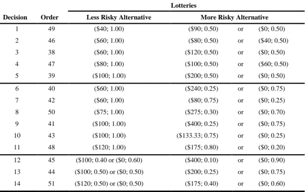
(18) We construct a set of dummy variables to use in subsequent analysis. Patient at 10, 50, 200, 380, and Patient never dummy variables are defined in the following manner, and imply distinct ranges of Individual Discount Rates (IDR) as shown: Patient at 10 = 1. Saved for all four decisions. IDR < 10%. Patient at 50 = 1. Saved for three decisions with interest ≥ 50. 10% < IDR ≤ 50%. Patient at 200 = 1. Saved for two decisions with interest rate ≥ 200%. 50% < IDR ≤ 200%. Patient at 380 = 1. Saved for one decision with interest rate = 380%. 200% < IDR ≤ 380%. Did not save for any decision. IDR ≥ 50%. Patient never = 1. While these discount rates are elicited over short time periods and appear high in absolute terms, we show in Eckel et al. (2005) that they are strongly correlated with discount rates measured over longer periods. Thus the dummy variables accurately capture relative differences across subjects in long-term discount rates. 3.2.c. Risk Preference Decisions. Participants’ attitudes toward risk were elicited using 14 pairs of lottery choices, shown in Table 6 below. The notation ($X; Y) means that X dollars is offered with probability Y; for example, in Decision 1, the participant is asked to choose between Option A yielding a certain $40, and Option B yielding a 50 percent chance of winning $90. The first 5 decisions involve a certain amount compared to a 50/50 gamble: for Decisions 2-5 the certain amount is equal to the expected value of the gamble. Decisions 6-11 also involve a choice between a certain amount and a gamble, varying probabilities from 50/50. Decisions 12-14 involve a choice between gambles.. Through these choices, subjects revealed their. preference for risk. This series of decisions with various payoffs and levels of risk can be used to explore the risk aversion of the participants.10. 10. Since this study was completed, a number of researchers have developed and tested tasks eliciting risk preferences. See for example, Holt and Laury (2002), Anderson et al., (2006), Eckel and Grossman (2008). 14.

(19) Table 5: Summary Description of the Risk-Preference Decisions Lotteries Decision. Order. 1. 49. Less Risky Alternative ($40; 1.00). ($90; 0.50). More Risky Alternative or. ($0; 0.50). 2. 46. ($60; 1.00). ($80; 0.50). or. ($40; 0.50). 3. 38. ($60; 1.00). ($120; 0.50). or. ($0; 0.50). 4. 47. ($80; 1.00). ($100; 0.50). or. ($60; 0.50). 5. 39. ($100; 1.00). ($200; 0.50). or. ($0; 0.50). 6. 40. ($60; 1.00). ($240; 0.25). or. ($0; 0.75). 7. 42. ($60; 1.00). ($80; 0.75). or. ($0; 0.25). 8. 50. ($75; 1.00). ($275; 0.30). or. ($0; 0.70). 9. 41. ($100; 1.00). ($400; 0.25). or. ($0; 0.75). 10. 43. ($100; 1.00). ($133.33; 0.75). or. ($0; 0.25). 11. 48. ($120; 1.00). ($175; 0.80). or. ($0; 0.20). 12. 45. ($100; 0.40 or ($0; 0.60). ($400; 0.10). or. ($0; 0.90). 13. 44. ($100; 0.50) or ($0; 0.50). ($200; 0.25). or. ($0; 0.75). 14. 51. ($120; 0.50) or ($0; 0.50). ($175; 0.40). or. ($0; 0.60). Notes: The notation ($X; Y) means that X dollars is offered with probability Y. The three pairs of decisions, (5, 13), (9, 12) and (11, 14), are common-ratio lotteries.. In Table 6, we show how the behavior of the participants, as described by a value between 0 and 14, was affected by the difference in the coefficient of variation (standard error/mean) between a pair of lotteries (the risk variable). The coefficient of variation is a measure of the riskiness of the lottery. (See Weber, et al., 2004 for a discussion of the superiority of this measure). Table 6: The Risk Factor Affecting the Percentage of Participants Choosing the Less Risky Lotteries for Each Risk Preference Decision (Logistic Specification) Variable Constant Riska. Coefficient 0.502 *** 1.194 ***. t-statistic 3.57 2.96. R 2 = 0.3731; 14 observations ________________________________________________________ *** indicate coefficients statistically significant at the 0.1 percent level. a Risk is the difference in the coefficients of variation (standard error/mean) between a pair of lotteries. A higher value of Risk means a higher difference in the level of risk between a pair of lotteries. (See Table 6 for a summary of the risk preference decisions.). A subset of the risky decisions was selected for creation of a variable for the regression analysis.. Five decisions involving a choice between a safe (certain) outcome and 50/50. alternative form the foundation of the measure RISK AVERSE. These decisions are intuitively. 15.

(20) easier for subjects to understand and restricting our attention to them reduced observed inconsistency. RISK AVERSE takes a value of one if subjects chose the safe option for at least three of the five simple risk decisions and a value of zero otherwise.. 3.3 Survey To complete the experiment, the subjects were asked to fill out an anonymous, 43question survey (ID numbers were used to link the survey and experimental decisions). The survey was designed with two purposes in mind. The first aim was to collect standard demographic information (such as sex, income, education, and main activity) to control for obvious socioeconomic differences in the sample. The second motivation was to collect surveybased measures of preferences and self-reported behavior to compare and contrast with the experimental measures. These measures included subjects’ self-perceived patience, risk aversion, locus of control, and savings behavior. The full set of questions is contained in Appendix A.. IV. Results:. 4.1 Analysis of Investment Decisions Given the right incentive, will the working poor save to invest in human capital? In this experiment, the decision to save is represented by a choice to forego a cash option offered by the experimenter in favor of an option to invest in one’s own human capital or a family member’s education. This section continues the investigation into the components of the investment decision. Regression analysis is used to simultaneously take into account the many factors that may influence an individual’s preference for assets. Demographic, behavioral, attitudinal, and treatment variables are considered. 4.2.1 Analysis of investment in one’s own human capital Consider four categories of investment preference for human capital: no preference for investment, some preference for investment, strong preference for investment, and very strong preference for investment. The latent variable IEi* captures the preference of individual i to invest in his or her own education. The following ordered probit has been estimated using a. 16.

(21) number of demographic and behavioral characteristics: IEi*  X i    i . Variable definitions and descriptive statistics are included in Appendix B and C. The preference for human capital investment is not directly observed, but rather we observe whether the subjects have chosen education when faced with three different trade-offs between cash and educational expenses. As a reminder, each subject made three choices during the experiment: $100 in cash vs. $200 in educational expenses, $100 in cash vs. $400 in educational expenses, and $100 in cash vs. $600 in educational expenses. Let the observed counterpart of the latent variable IEi* be defined as: IEi  0 if a participant never chose education for any trade-off; IEi  1 if education was chosen when $600 was offered in educational expenses (1 to 5 match rate); IEi  2 if education was chosen by the participant when at least $400 was offered in educational expenses (at least a 1 to 3 match rate); and finally,. IEi  3 if education was always the revealed choice of the participant for any offer of educational expenses. Assuming the error term is standard normally distributed,  i ~ N 0,1 then the probabilities y of participant i never choosing education, choosing education only once (at the 1 to 5 match rate), twice (when at least a 1 to 3 match rate is offered) and always choosing education are easily obtained as well as the corresponding likelihood function. The estimation results for the ordered probit are reported in Table 7. Greater patience results in a greater probability of choosing education over cash: at each discount rate level (indicated by the Patient variables) the probability of choosing education over cash increases. This is true for all except the highest discount rate category; Patient Never is the omitted category. This is consistent with the theory of human capital, as discussed in the introduction above. In addition, given their very low incomes, the extreme present-orientation of many of our subjects may be influenced by the subject’s degree of cash constraint, which also would lessen the appeal of long-term investments in human capital. More risk-averse subjects show a lower probability of investing in human capital. As was discussed in section 2, for the adult population in our sample, risk aversion implies a greater preference for the status quo, i.e., remaining in the workforce rather than investing in additional human capital. Many of the subjects in this experiment are likely to have endured failures in the labor market, school, and other situations. Investing in human capital carries a risk that they may want to avoid in order to steer clear of another possibility of failure. 17.

(22) Older persons are more likely to choose the cash alternative to education financing, reflecting the smaller time period available for recouping their investment in human capital. The effects of sex, number of children, and income levels are insignificant; that is, these factors do not enter directly into the determination of the investment in human capital. It is important to note that, by design, many of the subjects were below or near the LICOs and this result may simply indicate that individuals near the LICOs, whether above or below, act in a similar manner.. 18.

(23) Table 7: Determinants of Choosing Educational Expenses Over Cash (Ordered Probit, 219 Observations) Variable Names Patient at 10 Patient at 50 Patient at 200 Patient at 380 Risk Averse Age Risk Averse x Age Male Number Children Income Below LICO 120 Student Labor Force Constant δ1 δ2 Log likelihood Restricted Log Likelihood. Coefficient (t-statistic) 1.12 ***. (3.95) 1.02 (3.32) 0.76 (3.30) 0.31 (1.39) -1.66 (-2.65) -0.05 (-3.34) 0.04 (2.29) 0.02 (0.11) 0.02 (0.20) 0.01 (0.06) 0.23 (0.70) 0.25 (1.02) -1.35 (-2.09) 0.29 (4.94) 0.93 (9.24) -249.42 -272.57. *** ***. ** *** *. *. T-statistics are below each coefficient in parentheses. Bolded values indicate coefficients statistically significant on the 10 percent level, * indicates a 5 percent level, ** indicates a 1 percent level, and *** indicates a 0.1 percent level. Sample size of 219 resulted from 24 subjects dropped because of inconsistent time preference decisions and additional 13 subjects dropped because of inconsistent own education decisions.. The choice of education over cash is significantly related to patience, and to risk aversion, especially when it is interacted with age. The other demographic and behavioral variables are not significantly related to the decision to choose cash over education, and their addition does not change the pattern of results observed here.. 19.

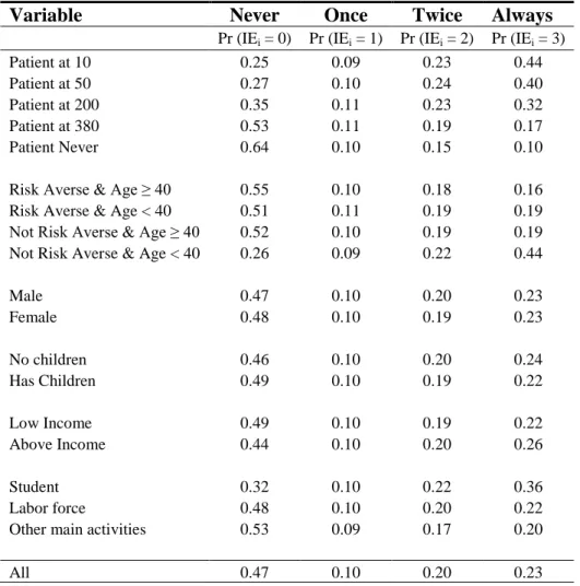
(24) Finally, and most importantly, the threshold parameters δ1 and δ2 indicate whether the different match rates affect the probability of investment in education at each level of subsidy. Positive, statistically significant coefficients indicate that different match rates offered to subjects induce different response rates, with higher subsidies producing larger responses. In Table 8, we have computed the predicted probability for each individual to be in each of the four categories of behavior (Never, Once, Twice, Always Chose Educational Expenses over cash). Then, for a specific characteristic, (Gender, income, etc.) an average conditional probability for each was computed. Table 8: Fitted Distribution of Number of Times Subject Chooses Education over Cash (never, once, twice, or three times) Variable. Never. Once. Twice. Pr (IEi = 0) 0.25 0.27 0.35 0.53 0.64. Pr (IEi = 1) 0.09 0.10 0.11 0.11 0.10. Pr (IEi = 2) 0.23 0.24 0.23 0.19 0.15. Pr (IEi = 3) 0.44 0.40 0.32 0.17 0.10. Risk Averse & Age ≥ 40 Risk Averse & Age < 40 Not Risk Averse & Age ≥ 40 Not Risk Averse & Age < 40. 0.55 0.51 0.52 0.26. 0.10 0.11 0.10 0.09. 0.18 0.19 0.19 0.22. 0.16 0.19 0.19 0.44. Male Female. 0.47 0.48. 0.10 0.10. 0.20 0.19. 0.23 0.23. No children Has Children. 0.46 0.49. 0.10 0.10. 0.20 0.19. 0.24 0.22. Low Income Above Income. 0.49 0.44. 0.10 0.10. 0.19 0.20. 0.22 0.26. Student Labor force Other main activities. 0.32 0.48 0.53. 0.10 0.10 0.09. 0.22 0.20 0.17. 0.36 0.22 0.20. All. 0.47. 0.10. 0.20. 0.23. Patient at 10 Patient at 50 Patient at 200 Patient at 380 Patient Never. Always. These results show that the level of impatience and the interplay between age and attitude towards risk both play an important role in the human capital investment decision. Note the 20.

(25) dramatic change in the probability of investment from subjects who exhibited relatively patient behavior (Patient at 10) to subjects who exhibited relatively impatient behavior (Never Patient) for the extreme investment preference category of Never. On average, 64 percent of the least patient subjects never chose to invest in education compared with only 25 percent of the most patient subjects. To a lesser degree than impatience, attitude towards risk coupled with age is also an important factor in the investment decision. On average, 55 percent of the more risk averse and older subjects never choose educational expenses over cash whereas only 26 percent of the young and risk accepting subjects exhibit this tendency. The younger, risk accepting subjects are also far more likely to always choose educational expenses. On average 44 percent choose educational expenses in all cases when offered in the experiment whereas their older and risk averse counterparts exhibited this behavior only 16 percent of the time. The results summarized in the last row of the table, ―All,‖ compare directly to the aggregate results. These average probabilities are unconditional on specific characteristics of participants and show the influence of the threshold parameters or match rates. Lastly, it is interesting to note that the standard deviations (not shown) are very low in columns 2 and 3 relative to columns 1 and 4 for each conditional characteristic. This suggests that the incentive effects of the match rates are very strong, as participants as a group, respond to changes in the generosity of the incentive. 4.2 Analysis of investment in family member’s education This section focuses on the preference to invest in the education of a family member. Just as the investment decision was modeled above, the latent variable, IFi* , of the following ordered probit captures the preference of individual i to invest in a family member’s education. The observed counterpart of the latent variable IFi* is defined as follows: IFi  0 if a participant never chose education for a family member for any trade-off offered; IFi  1 if education was chosen when $600 was offered in educational expenses (1 to 5 match rate);. IFi  2 if education was chosen by the participant when at least a 1 to 3 match rate was offered (that is $500 in education vs. $166 cash or $600 in education vs. $100 cash); and, finally, IFi  3 if education was always the revealed choice of the participant for any offer of educational expenses. 21.

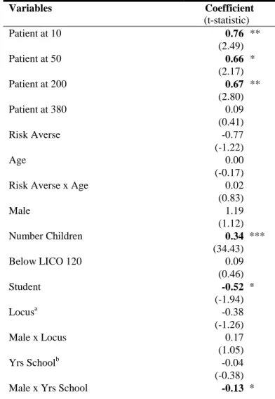
(26) The ordered probit (Table 9) was estimated using a number of demographic and behavioral characteristics as independent variables. As with the previous regression, the results show again that the threshold parameters are statistically significant and positive, indicating that subjects are responsive to the ―price‖ of saving for human capital. The number of children strongly affects this decision; people with children are substantially more likely to choose education of a family member, supporting our intuition that most subjects intended to use it as such. Another positive indicator of preference for savings for a family member’s education was belonging to a community group, a measure of the subjects’ connectedness to the neighborhood. The interaction of Male with years of schooling (Yrs School x Male) carries a negative coefficient, indicating that men with more schooling are actually more likely to choose cash over investment in a family member’s education. Table 9: Determinants of Choosing Education of a Family Member Over Cash (Ordered Probit, 220 Observations) Variables Patient at 10 Patient at 50 Patient at 200 Patient at 380 Risk Averse Age Risk Averse x Age Male Number Children Below LICO 120 Student Locusa Male x Locus Yrs Schoolb Male x Yrs School. Coefficient (t-statistic) 0.76 ** (2.49) 0.66 * (2.17) 0.67 ** (2.80) 0.09 (0.41) -0.77 (-1.22) 0.00 (-0.17) 0.02 (0.83) 1.19 (1.12) 0.34 *** (34.43) 0.09 (0.46) -0.52 * (-1.94) -0.38 (-1.26) 0.17 (1.05) -0.04 (-0.38) -0.13 * 22.

(27) Yrs School x Locus Local Community Organizationc Constant δ1 δ2 Log likelihood Restricted Log likelihood. (-1.83) 0.02 (1.11) 0.43 (1.65) 0.34 (0.23) 0.35 (5.30) 0.79 (8.11) -232.75 -258.60. T-statistics are below each coefficient in parentheses. Bolded values indicate coefficients statistically significant on the 10 percent level, * indicates a 5 percent level, ** indicates a 1 percent level, and *** indicates a 0.1 percent level. Sample size of 220 resulted from 24 subjects dropped because of inconsistent time preference decisions and additional 12 subjects dropped because of inconsistent family member education decisions. a Locus of Control is the Locus of Control index (0–7). A lower value indicates that the subject has strong feelings of self-efficacy. (Internal = 0, External =7) b Yrs School is the number of years of schooling. c For Local Community Organization a value of 1 indicates participants associated with; 0 if no affiliation. The membership of this group was almost exclusively Black. This is the closest approximation to a variable of visible minority status with the existing data.. The time preference measures enter the explanation for saving for a family member’s education much in the same way they helped explain some of the variation in investing in one’s own education. More patient participants are more likely to choose a family member’s education over a cash alternative. However, contrary to the previous ordered probit regression, attitude toward risk does not play a role in the choice to save for a family member’s education. This is in accordance with the interpretation given earlier to this variable with respect to investing in one’s own education: the education of a family member does not create a risky situation for the subject, as such. In Table 10 the estimated probabilities of investing in education of a family member for different subgroups are summarized. Note the differences in probabilities for saving for a family member’s education for subjects who exhibited relatively impatient behavior (Never Patient). Those individuals were far less likely to invest in family member’s education. Even when the match rate was most favorable, 1 to 5, on average close to 63 percent of the least patient subjects chose cash over the savings option. On average, only about 16 percent of the least patient would choose the savings option when their contribution would be matched at 100 percent (1 to 1).. 23.

(28) The results of the last line, ―All,‖ are unconditional on specific characteristics of participants and show the influence of the threshold parameters or match rates. As before, the standard deviations (not shown) of these estimated probabilities in columns two and three in Table 10 below are quite low, indicating the responsiveness of the participants to the different levels of subsidy.. Table 10: Fitted Distribution of Choosing Education of a Family Member over Cash.. Variable. Never. Once. Twice. Always. Pr (IFi = 0) 0.40 0.42 0.40 0.62 0.62. Pr (IFi = 1) 0.12 0.13 0.12 0.11 0.11. Pr (IFi = 2) 0.15 0.15 0.15 0.11 0.11. Pr (IFi = 3) 0.33 0.30 0.33 0.16 0.16. Risk Averse & age >=40 Risk Averse & Age < 40 Not Risk Averse & age >=40 Not Risk Averse & age <40. 0.46 0.61 0.40 0.42. 0.13 0.11 0.12 0.12. 0.15 0.11 0.15 0.14. 0.27 0.17 0.33 0.31. No children Local Community Organization No Local Community Organization. 0.62 0.32 0.56. 0.11 0.11 0.12. 0.11 0.15 0.12. 0.16 0.42 0.20. All. 0.53. 0.12. 0.13. 0.23. Patient at 10 Patient at 50 Patient at 200 Patient at 380 Patient never. V Validity Sixteen subjects of the 256 subjects received payment in the form of educational expenses.11 All sixteen subjects produced valid documentation to claim reimbursement for educational expenses within the specified time period of one year from the date of the experiment. This follow through does give an indication that subjects believed that they would be paid in the way described by the experimenters and made their decisions accordingly. This experiment was funded by the Social Research and Demonstration Corporation (SRDC) to provide input into the design of its field experiment testing the effect of subsidies to 11. There were 64 experimental decisions of which one was randomly chosen for payment. In order to receive payment in the form of educational expenses, a subject had to choose education expenses over the alternative offered and have that decision randomly chosen for payment. 24.

(29) saving for education. The experiment showed how subjects respond in a laboratory setting, and indicated that higher subsidies were substantially more effective in inducing subjects to choose education over cash, our proxy for the decision in the field to save for investment in human capital. SRDC began implementation of the field experiment, the learn$ave demonstration project, shortly after completion of this experiment. learn$ave is a random-assignment demonstration project. Participants are recruited for an information session. Generally speaking, with most random assignment projects, volunteers after the information session are randomly assigned into treatment groups and a control group. SRDC assigned volunteers to treatment groups that varied by province, match rate and financial counseling. As part of the implementation, SRDC conducted 36 focus groups on participants and non-participants across Canada. Of the project participants, separate focus groups were formed of those who saved regularly and those who did not save regularly. Their findings, published in the implementation report (2005) are strongly similar to our results and provide support for the validity of laboratory experiments in parameterizing policies. We highlight some of those similarities. We can compare the subjects in our experiment to the enrollees and non-participants in the learn$ave project. A majority of our experimental subjects had no knowledge about the education financing nature of the experimental choices until they arrived at the session. Therefore those subjects in our experiment that did not take up any education financing options can be compared to those that chose not to volunteer for learn$ave after they attended an information session. Those subjects that chose to take up education financing at different subsidy rates compare to those that that volunteered for learn$ave. In the executive summary of SRDC’s Design and Implementation Report, they conclude that learn$ave had much greater appeal for certain groups within the low-income population. Those who were ready for the changes in their lives that could be facilitated by participating in learn$ave and who were in a position to take advantage of these benefits were more likely to apply. Recent immigrants were foremost in this category, as many of them already had high levels of formal education and they needed to obtain Canadian credentials. In addition, learn$ave was of interest to Canadians who were more likely than the general eligible population to be younger, single, well educated, and employed. In our study, we found that younger, more educated and those engaged in the labor market were more likely to take up matched savings for educational expenses. 25.

(30) Of the learn$ave non-volunteers, there were many perceived barriers to applying. Some said that the savings period was too long. Some said the cap was too low to make the effort worthwhile.12 Some simply procrastinated in turning in their paperwork (SRDC, 2005 pp. 103107). These barriers can be captured in terms of time preference. In this experimental study, over 80 percent of the variation in the responses to the time preference decisions is explained by investment period, rate of return, and the absolute return, in the same directions found by the focus groups. Those in the experiment that were highly impatient were far less likely to take up any investment in human capital. Most interestingly, the SRDC report highlights personality differences but not visible differences between regular and irregular savers. For example, regular savers are forwardlooking; they are committed to make personal sacrifices; they have a clear savings goal; they have strong savings attitudes; they are self-disciplined. However, both regular and irregular savers cited low wages, unstable work or income and loss of employment as barriers to saving. Both lived through critical events, although regular savers were more able to protect savings in the face of such events. We have a strikingly similar result. We do not directly observe savings behavior in our experiment, but we do observe through the investment decisions who would be willing to forego near cash for future educational expense. The only visible characteristics listed in the regression summary in Table 10 that explain any of the variation in savings behavior is number of children. Our participants were not equally patient, and time preference, measured experimentally, enters strongly into the determination of probability of saving for a family member’s education as it does for saving for one’s own education.13. Time preference. observations are not typically collected but can potentially explain much of the behavioral differences between participants in a program like learn$ave.. VI. Summary and Conclusion This study makes novel use of experimental methodology to measure preferences and choices of the target population of a proposed government policy. The experiment was initiated to inform the design of the Canadian learn$ave project, which was promoted to encourage lowincome people to save money to increase their human capital. In this section we summarize the 12. The savings cap for a majority of learn$ave participants was $6000 with a match rate of $3 for every $1 saved. Explanations have been given in the literature to explain differences from person to person (see Becker and Mulligan, 1997, for a review and discussion). 13. 26.

(31) main findings of the study and their implications for a policy designed to induce the poor to save for investment in human capital – for themselves and for family members. Based on the experimental results, we conclude that a sizable proportion of the working poor would invest in human capital if the investment were sufficiently subsidized. The more the investment was subsidized, the more likely individuals were to invest. When subjects were presented with the opportunity analogous to the learn$ave matching offer ($400 in educational expenses or $100 in cash), 44 percent of subjects accepted the offer of education. Because these results entail giving up ―house money‖ rather than their own earned income, they may slightly overstate subjects’ willingness to forego current income for an investment in education.14 It is worth noting that for some people, investment in any form of asset seems to have been virtually ruled out: 16 percent of the subjects indicated no preference for any of the investment alternatives, even when the rate of return approached 500 percent. Many subjects were willing to delay consumption for substantial returns. Subjects were asked to choose between smaller payments sooner or larger payments later. For the participants of the experiment, choosing the larger payment later is analogous to saving. The subject must forego near-current consumption to receive future consumption. Delaying the sooner payoff – pushing it farther into the future – reduced the incentive to pick the later alternative even when the rate of return was held constant. More research is warranted, but these results suggest that savings programs that allow frequent withdrawals (to accelerate reward) and stress absolute difference in monetary gains as well as rate of return will fare much better than those that do not. When the stakes were high, these subjects were quite risk averse. Because many lowincome individuals, including a large fraction of our subjects, purchase lottery tickets, an action that is normally associated with risk-seeking attitudes, one might expect the poor to exhibit greater risk-seeking behavior in experimental games. The risk measures developed in this paper were not correlated to whether subjects bought lottery tickets, suggesting that attitudes toward risk might be more contextual than is often thought. In this experiment, the context of the monetary gambles offered as choices to the subjects had substantial stakes to be risked ($60 to. The house money effect hypothesizes that individuals take more risk with money they don’t yet consider to be their own. 14. 27.

(32) $120) for modest gains. This is perhaps a better indicator of one’s risk aversion to educational investment than the mere observation of behavior towards lottery ticket purchases.15 These two experimentally measured characteristics, patience and risk aversion, help us to inform the larger question: Will the working poor save to invest in human capital? The more patient participants were, the more likely they were to invest in their own education. The more risk-averse subjects were, the less likely they were to invest in their own education. These subjects viewed foregoing certain cash in exchange for a multiple of that cash in own educational expenses as a risky alternative. In addition, younger subjects were more likely to invest in education.16 Perhaps those with recent education experience were better able to assess the risk involved in an investment in education. The decision to save for a family member’s education is somewhat different from that of investing in one’s own education. Again, patient participants were more likely to save for a family member’s education, but in contrast to investing in one’s own education, a subject’s attitude towards risk played no role. The education of a family member does not involve a risky situation for the subject, as such. Two behavioral characteristics, patience and attitude towards risk, are key to understanding the determinants of educational investment for the low-income individuals in this experiment. More research is needed to understand the structure of the risk in investing in education and the factors that can induce one to be more patient in waiting for compensation.. 15. For example, Holt and Laury (2002) show that higher stakes increase risk aversion in a convenience sample of student subjects, particularly for male participants. 16 This is shown in Tables 3 and 8, comparing student to all. The student variable is, however, insignificant in the ordered probit of Table 7. They are a relatively small part of the sample, representing only 12%. 28.

(33) References Andersen, S., Harrison, G., Lau, M., Rutström, E., 2006. Elicitation using multiple price list formats. Experimental Economics 9, 383-405. Bound, J., Turner, S., 2002. Going to war and going to college. Journal of Human Resources 20, 784-815. Becker, G., Mulligan, C., 1997. The endogenous determination of time preference. Quarterly Journal of Economics 112 , 729-58. Burks, S., Carpenter, J., Goette, L., Rustichini, A., 2008. Cognitive skills explain economic preferences, strategic behavior, and job attachment. IZA Discussion Paper No. 3609. Cameron, S., Heckman, J., 1998. Life cycle schooling and dynamic selection bias: Models and evidence for five cohorts of American males. Journal of Political Economy 106, 262-333. Chen, Stacey. H., 2002. Is investing in college education risky? Working paper, Department of Economics, State University of New York at Albany. Dynarski, S., 2002. The behavioral and distributional implications of aid to college. American Economic Review 92, 279-85. Eckel, C., Grossman, P., 2008. Forecasting risk attitudes: An experimental study using actual and forecast gamble choices. Journal of Economic Behavior and Organization 68, 1-17. Eckel, C., Johnson, C., Montmarquette, C., 2002. Will the working poor invest in human capital? A laboratory experiment. Working paper 02-01, Social Research and Demonstration Corporation, (http://www.srdc.org/uploads/workingpoor.pdf) Eckel, C., Johnson, C., Montmarquette, C., 2005. Saving decisions of the working poor: Short and long-term horizons. Research in Experimental Economics, Volume 10: Field Experiments in Economics, edited by J. Carpenter, G. Harrison, J. List. Eckel, C., Johnson, C., Montmarquette, C., Rojas, C., 2007. Debt aversion and the demand for loans for post-secondary education. Public Finance Review 35, 233-262. Frederick, S., Loewenstein, G., Donoghue, T.O., 2002. Time discounting and time preference: A critical review. Journal of Economic Literature XL, 351-401. Harrison, G., W., Lau, M.I., Williams, M.B., 2002. Estimating individual discount rates in Denmark: A field experiment. American Economic Review 92, 1606-1617. Holt, C.A., Laury, S., 2002. Risk aversion and incentive effects. American Economic Review 92, 1644-1655.. 29.

(34) Heckman, J.J., Lochner, L.J., Todd, P.E., 2008. Earnings functions and rates of retrurn. Journal of Human Capital 2, 1-31. Keane, M.P., 2002. Financial aid, borrowing constraints and college attendance: Evidence from structural estimates. American Economic Review, Papers and Proceedings 92, 293-97. Keane, M.P., Wolpin, K.I., 2000. Eliminating race differences in school attainment and labor market success. Journal of Labor Economics 18, 614-52. Kingwell, P., Dowie, M., Holler, B., Vincent, C., Gyarmati, D., Cao, H., 2005. Design and implementation of a program to help the poor save: The learn$ave project. Social Research and Demonstration Corporation (http://www.srdc.org/uploads/learnsave_implementation.pdf). Laibson, D. I., Repetto, A., and Tobacman, J., 1998. Self-control and saving for retirement. Brookings Papers on Economic Activity 1, 91–196. Levhari, D. Weiss, Y., 1974. The effect of risk on the investment in human capital. American Economic Review 64, 950-963. Loewenstein, G., Thaler, R., 1989. Anomalies: Intertemporal choice. The Journal of Economic Perspectives 3, 181–93. O’Donoghue, T., Rabin, M., 2001. Choice and procrastination. Quarterly Journal of Economics 116, 121-160. Roth, A., 2002. The economist as engineer: Game theory, experimentation, and computation as tools for design economics. Econometrica 70, 1341-78. Samuelson, P., 1937. A note on the measurement of utility. Review of Economics Studies 4, 155-161. Statistics Canada, Low-income division, 2001. Low income cutoffs from 1991-2000. Publication # 75F0002MIE – 01007. Stefor, N., Turner, S., 2002. Back to school: Federal student aid policy and adult college enrollment. Journal of Human Resources 37, 336-52. Weber, E., Shafir, S., Blais, A-R., 2004. Predicting risk-sensitivity in humans and lower animals: Risk as variance or coefficient of variation. Psychological Review 111, 430-455. Weiss, Y., 1972. The risk element in occupational and educational choices. Journal of Political Economy 80, 1203-1213.. 30.

(35) Appendix A Materials Related to the Experiment ”Human Capital Investment by the Poor: Informing Policy with Laboratory and Field Experiments”. 1.

(36) 48. Instructions The rules: 1. You are asked to complete two questionnaires. The first questionnaire (64 questions) is made of choice questions. The second questionnaire (43 questions) is made of information questions. All answers will be treated confidentially. 2. You win at least $12, but you can make a great deal more. 3. You must answer each question, without exception. This is the only way to win a prize. 4. If you have any questions once you have started answering the questionnaire, please raise your hand, and someone will help you. The payment procedure: Once you have answered all the questions in the survey, you will be invited to meet with me to determine the prize you win. This prize will be determined in the following manner: 1. A ball will be drawn randomly from an urn containing 64 balls, numbered from 1 to 64 representing all the choice questions of the survey. The urn does not include balls for the information questions. 2. The ball drawn identifies the question that determines your prize following your choice at that question. 3. Some monetary prizes will be given in cash, others will be mailed at a specific date. You will have to sign a receipt. In the cases of non-monetary prizes, you will receive an IOU certificate and your prize will be delivered to you by a special courier in the first weeks of January. A practice questionnaire: 1. To familiarise you with the types of choice questions of the survey, you are invited to answer 6 questions (numbered 1 to 6) of a training questionnaire. 2. Once this is done by all participants, we will draw a few balls from the urn to illustrate the payment procedure.  The whole survey should take less than 90 minutes to be completed.  Please note that there is no wrong or right answer, we want to know what YOU think..