Modeling Preferences for Ambiguous Utterance Interpretations

(1)

HAL Id: tel-01908642

https://hal.archives-ouvertes.fr/tel-01908642v2

Submitted on 8 Jul 2019

HAL is a multi-disciplinary open access archive for the deposit and dissemination of sci-entific research documents, whether they are pub-lished or not. The documents may come from teaching and research institutions in France or abroad, or from public or private research centers.

L’archive ouverte pluridisciplinaire HAL, est destinée au dépôt et à la diffusion de documents scientifiques de niveau recherche, publiés ou non, émanant des établissements d’enseignement et de recherche français ou étrangers, des laboratoires publics ou privés.

Interpretations

Mehdi Mirzapour

To cite this version:

Mehdi Mirzapour. Modeling Preferences for Ambiguous Utterance Interpretations. Other [cs.OH]. Université Montpellier, 2018. English. �NNT : 2018MONTS094�. �tel-01908642v2�

(2)

THÈSE POUR OBTENIR LE GRADE DE DOCTEUR

DE L’UNIVERSITÉ DE MONTPELLIER

En Informatique

École doctorale Information, Structures et Systèmes Unité de recherche LIRMM

Présentée par Mehdi MIRZAPOUR

Le 28 septembre 2018

Sous la direction de Pr. Christian RETORÉ

et Dr. Jean-Philippe PROST

Devant le jury composé de

Pr Veronica DAHL, Professeur, Université de Simon Fraser Pr Christophe FOUQUERÉ, Professeur, Université Paris 13, LIPN Dr Maxime AMBLARD, MCF HDR, Université de Lorraine LORIA Dr Philippe BLACHE, Directeur de Recherche, CNRS LPL Pr Violaine PRINCE, Professeur, Université de Montpellier LIRMM Dr Jean-Philippe PROST, MCF, Université de Montpellier LIRMM Pr Christian RETORÉ, Professeur, Université de Montpellier LIRMM

Rapporteur Rapporteur Examinateur Examinateur Examinateur Co-directeur Directeur

Modeling Preferences for

(3)

(4)

Declaration of Authorship

I, Mehdi MIRZAPOUR, declare that this thesis titled, “Modeling Preferences for Am-biguous Utterance Interpretations” and the work presented in it are my own. I con-firm that:

• This work was done wholly or mainly while in candidature for a research de-gree at this University.

• Where any part of this thesis has previously been submitted for a degree or any other qualification at this University or any other institution, this has been clearly stated.

• Where I have consulted the published work of others, this is always clearly attributed.

• Where I have quoted from the work of others, the source is always given. With the exception of such quotations, this thesis is entirely my own work.

• I have acknowledged all main sources of help.

• Where the thesis is based on work done by myself jointly with others, I have made clear exactly what was done by others and what I have contributed my-self.

Signed: Date:

(5)

(6)

“Like a sword, a word can wound or kill, but as long as one does not touch the blade, the sword is no more than a smooth piece of metal. Someone who knows the qualities of a sword does not play with it, and someone who knows the nature of words does not play with them.” Miyamoto Musashi

(7)

(8)

UNIVERSITY OF MONTPELLIER

Abstract

Computer Science LIRMM Doctor of Philosophy

Modeling Preferences for Ambiguous Utterance Interpretations

by Mehdi MIRZAPOUR

The problem of automatic logical meaning representation for ambiguous natural language utterances has been the subject of interest among the researchers in the do-main of computational and logical semantics. Ambiguity in natural language may be caused in lexical/syntactical/semantical level of the meaning construction or it may be caused by other factors such as ungrammaticality and lack of the context in which the sentence is actually uttered. The traditional Montagovian framework and the family of its modern extensions have tried to capture this phenomenon by providing some models that enable the automatic generation of logical formulas as the meaning representation. However, there is a line of research which is not pro-foundly investigated yet: to rank the interpretations of ambiguous utterances based on the real preferences of the language users. This gap suggests a new direction for study which is partially carried out in this dissertation by modeling meaning prefer-ences in alignment with some of the well-studied human preferential performance theories available in the linguistics and psycholinguistics literature.

In order to fulfill this goal, we suggest to use/extend Categorial Grammars for our syntactical analysis and Categorial Proof Nets as our syntactic parse. We also use Montagovian Generative Lexicon for deriving multi-sorted logical formula as our semantical meaning representation. This would pave the way for our five-fold contributions, namely, (i) ranking the multiple-quantifier scoping by means of un-derspecified Hilbert’s epsilon operator and categorial proof nets; (ii) modeling the semantic gradience in sentences that have implicit coercions in their meanings. We use a framework called Montagovian Generative Lexicon. Our task is introduc-ing a procedure for incorporatintroduc-ing types and coercions usintroduc-ing crowd-sourced lexi-cal data that is gathered by a serious game lexi-called JeuxDeMots; (iii) introducing a new locality-based referent-sensitive metrics for measuring linguistic complexity by means of Categorial Proof Nets; (iv) introducing algorithms for sentence comple-tions with different linguistically motivated metrics to select the best candidates; (v) and finally integration of different computational metrics for ranking preferences in order to make them a unique model.

(9)

(10)

Acknowledgements

Firstly, I would like to express my sincere gratitude to my advisors Christian Retoré and Jean-Philippe Prost for being willing to take me as a student and also for their continuous and extraordinary support of my Ph.D study, for their patience, motivation, and immense knowledge. I will be forever grateful for their help.

Besides my advisors, I would like to appreciate Philippe Blache and Richard Moot for their kind support and the time that they spent to discuss novel ideas. I am profoundly influenced by their research style and wise approaches. My sincere thanks also go to Violaine Prince, Mathieu Lafourcade, Bruno Mery, Davide Catta and Alain Joubert who provided patiently discussions and hints during my research in TEXTE group. I would like to express my gratitude for Jan van Eijck and Christina Unger for introducing their invaluable book entitled Computational Semantics with Functional Programming which inspired me to enter to the field of Computational Se-mantics.

I would like to thank my Ph.D. committee members Maxime Amblard, Philippe Blache, Veronica Dahl, Christophe Fourqueré and Violaine Prince for their insight-ful comments and constructive ideas which deserve further attention for my future research and also my internal supervision committee Madalina Croitoru, David De-lahaye and I2S doctoral school responsible Marianne Huchard. I appreciate very supportive and professional administration members of our lab Elisabeth Greverie, Cecile Lukasik, Guylaine Martinoty and Nicolas Serrurier. I thank my fellow lab-mates Jimmy Benoits, Davide Catta, Maxime Chapuis, Nadia Clairet, Kévin Cousot, Lionel Ramadier and Noémie-Fleur Sandillon-Rezer for their stimulating discus-sions. Also, I thank my ex-supervisors Gholamreza Zakiani and Fereshteh Nabati for paving the way for my Ph.D.with providing support and encouragement for the continuation of my study before and after starting my PhD. I am grateful to Ferey-doon Fazilat for enlightening the first glance of logical study. I am also grateful to Gyula Klima for sharing his insightful ideas on logic, language and semantics and also for his kind support of my Ph.D. applications.

I would also like to thank the following people for their support, ideas and lec-tures that have influenced me: Ali-Akbar Ahmadi Aframjani, Fabio Alves, Lasha Abzianidze, Jean-Yves Béziau, Patrick Blackburn, Johan Bos, Adrian Brasoveanu, Michael Carl, John Corcoran, Stergios Chatzikyriakidis, Robin Cooper, Alexander Dikovsky, Jakub Dotlaˇcil, George Englebretsen, Edward Gibson, Jean-Yves Girard, Philippe De Groote, Hans Götzsche, Mohammad-Ali Hojati, Rodrigo Guerizoli, Herman Hendriks, Mark Johnson, Joachim Lambek, Anaïs Lefeuvre, Victoria Lei, Defeng Li, Roussanka Loukanova, Zhaohui Luo, Laura Kallmeyer, Vedat Kamer, Ron Kaplan, Amirouche Moktefi, Friederike Moltmann, Glyn Morrill, Larry Moss, Reinhard Muskens, Lotfollah Nabavi, Katashi Nagao, Petya Osenova, Moham-madreza A. Oskoei, Terence Parsons, Wiebke Petersen, James Pustejovsky, Aarne Ranta, Stephen Read, Mehrnoosh Sadrzadeh, Moritz Schaeffer, Jeremy Seligman, Kiril Simov, Mark Steedman, Jakub Szymanik, Simon Thompson, Erik Thomsen,

¸Safak Ural, Shravan Vasishth and Yorick Wilks.

Last but not the least, I would like to thank my wife Fatemeh, my children Iliya and Mélodie, my parents, my sisters and my friends for supporting me spiritually throughout writing this thesis.

(11)

(12)

List of Figures

2.1 Local Trees of the Polar Category Formulas . . . 7

2.2 The polar categorial tree of ((np/S)/(np/S))⊥ . . . 8

2.3 The categorial proof-net analysis for the example "Every barber shaves himself." . . . 9

2.4 The categorial proof-net analysis with labels for the example "Every barber shaves himself." . . . 11

2.5 Polymorphic conjunction: P( f (x))&Q(g(x)) with x ∶ ξ, f ∶ ξ → α, g ∶ ξ → β. . . . 15

2.6 A part of the JDM network (taken form [LJ15]). . . 18

2.7 Screen-shot of an ongoing game with the target verb fromage (cheese) (taken form [Cha+17a]). . . 19

2.8 Screen-shot of the game result with the target noun fromage (taken from [Cha+17a]). . . 20

3.1 Proof net analyses for 3.3a (left hand) and 3.3b (right hand) with the relevant profiles. . . 24

3.2 Proof net analyses for reading (a) of the example 3.4a. . . 27

3.3 Proof net analyses for reading (b) of the example 3.4b. . . 28

3.4 Proof net analyses for reading (c) of the example 3.4c. . . 29

3.5 Proof net analyses for reading (d) of the example 3.4d. . . 30

3.6 Proof net analyses for reading (e) of the example 3.4e. . . 31

3.7 Proof net analyses for 3.6a (left hand) and 3.6b (right hand) with the relevant profiles. . . 32

3.8 New procedure for the example 3.6 . . . 35

4.1 Obtaining Coercions: General Scheme, Query Code and Outcome Ta-ble for Example (a) . . . 49

4.2 Obtaining Coercions: General Scheme, Query Code and Outcome Ta-ble for Example (b) . . . 51

5.1 IDT-based Complexity Profiles for 5.3a and 5.3b. . . 57

5.2 Proof net analyses for 5.3a (subject-extracted relative clause). . . 58

5.3 Proof net analyses for 5.3b (object-extracted relative clause). . . 59

5.4 Accumulative DLT-based Complexity Profiles for 5.3a and 5.3b. . . 61

5.5 Proof net analysis for the example 5.4a. . . 62

5.6 Accumulative DLT-based Complexity Profiles for 5.4a and 5.4b. . . 62

5.7 Proof net analysis for the example 5.4b. . . 63

5.8 Accumulative DLT-based Complexity Profiles for 5.5a and 5.5b . . . . 64

5.10 Proof net analyses for 5.5a located in top (first attempt reading) and 5.5b in bottom (full garden path sentence). . . 65

5.11 Proof net analyses for 5.6a (object relativization). . . 66

5.12 Proof net analyses for 5.6b (subject relativization). . . 67

5.9 Accumulative DLT-based Complexity Profiles for 5.6a and 5.6b . . . . 68

(17)

5.14 Proof net analyses for 5.7 with middle adverbal attachments. . . 70

5.15 Proof net analyses for 5.7 with lowest adverbal attachments. . . 71

5.16 Accumulative DLT-based complexity profiles for three readings of 5.7 71 5.17 Proof net analyses for 5.8 with sensical (left) and nonsensical (right) interpretations. . . 72

5.18 Accumulative DLT-based complexity profiles for two readings of 5.8 . 72 5.19 Proof net analyses for 5.9a . . . 73

5.20 Proof net analyses for 5.9b . . . 74

5.21 Accumulative DLT-based complexity profiles for 5.9a and 5.9b . . . . 74

6.1 Possible structural trees of a sequence w1w2w3 . . . 82

6.2 Three possible structural trees for the example 6.2 . . . 84

6.3 Proof net analyses for 6.6a and 6.6b. . . 99

6.4 Proof net analysis for 6.7a. . . 102

6.5 Proof net analysis for 6.7b. . . 103

6.6 Proof net analysis for 6.7b with the weights. . . 105

6.7 Proof net analysis for 6.9a with the (violation) weights. . . 108

6.8 Proof net analysis for 6.9b with the (violation) weights. The violation weights with the light-colored axioms have the value ’1’; the rest, i.e. the dark-colored axioms have the value ’0’ . . . 109

6.9 Proof net analysis for 6.9c with the (violation) weights. The violation weights with the light-colored axioms have the value ’1’; the rest, i.e. the dark-colored axioms have the value ’0’ . . . 110

6.10 Proof net analysis for 6.9d with the (violation) weights. The violation weights with the light-colored axioms have the value ’1’; the rest, i.e. the dark-colored axioms have the value ’0’ . . . 111

6.11 Proof net analysis for 6.9e with the (violation) weights. The violation weights with the light-colored axioms have the value ’1’; the rest, i.e. the dark-colored axioms have the value ’0’. . . 112

7.1 Proof net analysis for 7.1a. . . 120

7.2 Proof net analysis for 7.1b. . . 121

7.3 The General Scheme for Integrating the Rankings. . . 122

(18)

List of Tables

2.1 Sequent calculus rules for LC . . . 6

6.1 Unification of variable categories and fixed (learned) categories . . . . 82

6.2 Unification of variable types and learned types . . . 84

6.3 Step (1) of parsing with unification for the example 6.3 . . . 85

6.6 Last step of parsing with unification for the example 6.3 . . . 86

6.7 Parsing with unification for the example 6.6 . . . 97

6.8 Parsing with unification for the example 6.6 . . . 98

6.9 Calculation of the incomplete dependency number for 6.6a and 6.6b. . 98

6.10 Calculation of the dependency locality number for 6.6a and 6.6b. . . . 98

6.13 Calculation of the activation-based complexity measurement for 6.7a and 6.7b. . . 104

B.1 Calculation of the incomplete dependency number for 3.3a and 3.3b. . 145

B.4 Calculation of the dependency locality number for 5.3a and 5.3b. . . . 145

B.8 Calculation of the dependency locality number for the readings of 5.7. 146 B.9 Calculation of the dependency locality number for the readings of 5.8. 146 B.10 Calculation of the dependency locality number for 5.9a and 5.9b. . . . 146

B.15 Calculation of the activation-based complexity measurement for 6.7a and 6.7b. . . 147

(19)

(20)

List of Abbreviations

CG Categorial Grammar

CHR Constraint Handling Rules

CPN Categorial Proof Net

DLT Distance Locality Theory

GSC Gentzen Sequent Calculus

GWAP Games With A Purpose

IDT Incomplete Dependency Theory

JDM Jeux De Mots

LC Lambek Calculus

MGL Montagovian Generative Lexicon

MLL Multiplicative Linear Logic

(21)

(22)

(23)

(24)

Chapter 1 Introduction

To know ten thousand things, know one well.

Miyamoto Musashi

Ambiguity is an important linguistic phenomenon which demands a compu-tational treatment in almost all of the subfields of natural language processing, such as Information Retrieval, Sentiment Analysis, Machine Translation, Question-Answering and Natural Language Understanding. The ambiguity may be caused in lexical/ syntactical/ semantical level of meaning construction or it may be caused by other factors such as ungrammaticality or the absence of the context in which the sentence is actually uttered.

In computational formal semantics, the problem of automatic meaning repre-sentation for ambiguous natural language utterances has been extensively studied. More specifically, in Montagovian-style formal semantic frameworks one would be able to derive meanings from a given ambiguous text in a systematic and straight-forward approach.

A natural, and yet plausible question that can be raised in the computational formal semantic field is that how different possible meaning representations of a written or spoken utterance might be quantitatively ranked in alignment with the well-studied human preferential performance theories.

This question is not just interesting from a computational linguistic or computa-tional psycholinguistic perspective. It is important due to this fact that some compu-tational frameworks over-generate meaning structures and this necessarily suggests a ranking mechanism to rule out some of them. Even if a computational framework properly generates meanings for ambiguous utterances, ranking them as close as possible to the human performance phenomena would be an interesting task. This would provide a quantitative account in favor of introducing new metrics for the fu-ture studies in humanizing the natural language understating, i.e. making machines that understand natural language similar to humans. Those machines are supposed to obtain the meaning of linguistically ambiguous utterances in a way that makes the communication between human and machines smoothly. Obviously, the prob-lem of the misunderstanding between machines and humans would increase when no human-like computational ranking is available.

The main question of this dissertation is how to fill the mentioned gap by pro-viding meaning preferential models for ambiguous utterances in alignment with some of the well-studied human preferential performance theories available in the linguistics and psycholinguistics literature. There are more specific questions which

(25)

are clustered around the main general question, such as: How can the problem of the ranking multiple-quantifier sentence be efficiently addressed? How can we have the preferential models for those human preferences which are constrained by the lexical data? How can we use human knowledge in lexical-semantic networks to address the previous question? What is a suitable and proper representation of the sentence meaning? How would these meaning representations pave the way to adopt the modern computational psycholinguistic theories into our ranking algorithms? How can we rank ambiguous incomplete sentences? How can potential interpretations for incomplete sentences quantitatively be ranked as close as possible to human prefer-ences?

Although, our research objectives cover the linguistic phenomena which, in prin-ciple, is tied up with the ambiguity problem, we will go beyond the classical prob-lem of ranking the ambiguous utterances, and we discover novel solutions for other linguistic phenomena such as quantifier scoping, the gradient of semanticality, em-bedded pronouns, garden pathing, unacceptability of center emem-bedded, preference for lower attachment and passive paraphrases acceptability. In order to fulfill this, we use Categorial Grammars for our syntactical analysis and Categorial Proof Nets as our syntactic parse. We also use Montagovian Generative Lexicon for deriv-ing multi-sorted logical formula as our semantical meanderiv-ing representation. Thanks to the Curry–Howard isomorphism and the semantic readings on proof nets, the syntax-semantics interface will be quite straightforward. It is worth mentioning that the meaning can be represented as multi-sorted higher-order logical formulas. Also, it is straightforwardly possible to reify the higher-order logical meaning repre-sentations in alignment with the event semantics in Davidsonian [Dav67] and neo-Davidsonian proposals [Res67; Par90].

Our hypothesis is that by applying the above methodology we can quantitatively model a number of linguistic performance phenomena. Our computational model supports the human performances that are experimentally verified by modern psy-cholinguistic theories.

This work is organized as follows:

In chapter 2, we provide an overview of the background knowledge that one needs to understand this dissertation. It starts with Lambek Calculus as our syntac-tic analysis with the essential definitions and exploring Lambek Sequent Calculus. Then, we highlight the problem of spurious ambiguity that exist in the sequent cal-culus. After that, we explain how Categorial Proof Nets can overcome the spurious ambiguity problem. We also go through all the needed definitions, technicalities and examples that is needed to grasp categorial proof-net and the semantic readings of it. Then, we explicate Montagovian Generative Lexicon and its lexicon organi-zation. We discuss how representing meaning as multi-sorts higher order logic can help us to capture coercion and co-prediction in the language. We end up this chap-ter with introducing JeuxdeMots, a French lexical-semantic network. The relevant graph structures and the validation process would be generally overviewed.

In chapter 3, we focus on the problem of ranking the valid logical meanings of a given multiple-quantifier sentence only by considering the syntactic quantifier or-der. We first report some deficiencies that exist in an existing state-of-the-art tech-nique (for solving the problem of quantifier scope ranking) known as Incomplete Dependency-based Complexity Profiling [Mor00]. One of the main problem with

(26)

this approach is that it does not properly support the ranking problem in some of the sentences such as sentence-modifier adverbials, nested sentences and direct speech. We try to fix this problem by defining a new metric which is inspired by Hilbert’s epsilon and introducing the notion of the reordering cost. We will see how this gives a correct account in favour of the problematic cases.

In chapter 4, we focus on the semantic gradiences that potentially happens in sentences that have implicit coercions in their linguistic meaning. The aim of this study is to find an automatic treatment for this kind of semantic preferences and to capture it in our modeling. In order to perform such a task we need to have a rich lexical information. Frameworks based on Generative Lexicon theories [Pus91] such as Motagovian Generative Lexicon [Ret14], can have a rich logical representation using a Montague-like compositional process. A crucial problem for these systems is then to have sufficient lexical resources (as a rich lexicon incorporating types and coercions) to function. Our main task in this chapter is introducing a procedure which can build such a lexicon for the Montagovian Generative Lexicon. We will do this task by using crowd-sourced lexical data that is gathered by a serious game which is called JeuxDeMots. The frequencies of the lexical occurrences— which is automatically gathered by the game players— would play a key role in our ranking mechanism. Our strategy, following [FW83], would be based on a mechanism called preference-as-procedure. We practice such a strategy for automatic treatment of se-mantic gradience in our computational modeling.

In chapter 5, we provide a quantitative computational account of why such a sen-tence has a harder parse than some other sensen-tence, or that one analysis of a sensen-tence is simpler than another one. We take for granted the Gibson’s results on human pro-cessing complexity. Gibson first studied the notion of the nesting linguistic difficulty [Gib91] through the maximal number of incomplete syntactic dependencies that the processor has to keep track of during the course of processing a sentence. We re-fer to this theory as Incomplete Dependence Theory (IDT) as coined by Gibson. IDT had some limitations for the referent-sensitive linguistic phenomena, which justified the later introduction of the Syntactic Prediction Locality Theory [Gib98]. A vari-ant of this theory, namely Dependency Locality Theory (DLT), was introduced later [Gib00] to overcome the limitations of IDT against the new linguistic performance phenomena. In the original works, both IDT and DLT use properties of linguis-tic representations provided in Government-Binding Theory [Cho82]. We provide a new metric which uses (Lambek) Categorial Proof Nets. In particular, we cor-rectly model Gibson’s account in his Dependency Locality Theory. The proposed metric correctly predicts some performance phenomena such as structures with em-bedded pronouns, garden pathing, unacceptability of center emem-bedded, preference for lower attachment and passive paraphrases acceptability. Our proposal extends existing distance-based proposals on Categorial Proof Nets for complexity measure-ment while it opens the door to include semantic complexity, because of the syntax-semantics interface in categorial grammars. The purpose of developing our putational psycholinguistic model is not solely limited to measuring linguistic com-plexity.

In chapter 6, we work on incomplete utterances with missing categories. In the first place, we introduce two algorithms for resolving incomplete utterances. The first algorithm is based on AB grammars, Chart-based Dynamic Programming and learning Rigid AB grammars with a limited scope of only one missing category which have O(n4) time complexity (n is the number of the words in a sentece). The

(27)

second algorithm employs Constraint Handling Rules which deals with k > 1 miss-ing categories which enable us to find more than one missmiss-ing categories at cost of the exponential complexity. In the second place, we introduce measurements on the fixed categorial proof nets motivated by Gibson’s distance-based theories, Violation Ratio factor and Activation Theory.

In chapter 7, we focus on the problem of integration different computational met-rics for ranking preferences in order to make them a unique model. We see this prob-lem similar, to some extent, to the probprob-lem of aggregation of the preferences. In other words, we provide a procedure to make preference over different linguistic prefer-ences introduced throughout this dissertation. We mainly use the lexicographical ordering for aggregating the different preferences. We see this computational pro-cedure with a number of running examples. In chapter 8 we draw conclusions and discuss avenues for further works.

(28)

Chapter 2 Background Knowledge

You should not have any special fondness for a particular [tool], or anything else, for that matter. Too much is the same as not enough. Without imitating anyone else, you should have as much [tools] as suits you.

Miyamoto Musashi

In this chapter, we introduce the background knowledge that is assumed one would need to understand this dissertation.1 The underlying concepts and the no-tations within each exploited framework are described. This should not prevent the non-familiar readers to consult the relevant references in each section for detailed information since this chapter is not meant to explicate briefly each framework in a lengthy manner.2

2.1 Lambek Calculus

Lambek calculus(LC) is introduced for the first time by Lambek in his seminal paper [Lam58]. The motivation behind this system is to provide a resource-boundedness logic in favor of syntactical parsing under the slogan ’parsing as a deduction’. We provide an overview of the existing material [MR12b] on Lambek Calculus.

Definition 2.1. The category formulas (Lp) are freely generated from a set of usual

syntactical primitive types P = {S, np, n, pp, ⋯} by directional divisions, namely the binary infix connectives / (over), / (under) and ● (product) as follows:

Lp ∶∶= P ∣ (Lp/Lp) ∣ (Lp/Lp) ∣ (Lp●Lp)

Note that A/B and B/A have also some intuitive interpretations. An expression of type A/B (resp. B/A) when it looks for an expression of type A on its left (resp. right) forms a compound expression of type B. An expression of type A followed by an expression B is of type A ● B, and the product is related to / and / by the following relations:

A/(B/X) = (B ● A)/X (X/A)/B = X/(B ● A)

1_{We assume that the readers have some familiarity with the Typed Lambda Calculus and} Intu-itionistic Propositional Calculus. Interested readers can consult [HS80; GTL89] for more details on the subject.

(29)

Definition 2.2. A sequent, Γ ⊢ A, comprises formula A as succedent and Γ a se-quence of finite formulas as antecedent. The table 2.1 shows the rules of LC which is provided in Gentzen Sequence Calculus in which A, B and C are formulas, while Γ_{, Γ}′_{and ∆ are sequences which each contains finite formulas:}

Γ_{, B, Γ}′ _⊢_C _{∆ ⊢}_A Γ_{, ∆, A/B, Γ}′⊢_C /h A, Γ ⊢ C Γ ⊢A/C /i Γ ≠ǫ Γ_{, B, Γ}′ _⊢_C _{∆ ⊢}_A Γ_{, B/A, ∆, Γ}′⊢_C /h Γ_{, A ⊢ C} Γ ⊢C/A /i Γ ≠ǫ Γ_{, A, B, Γ}′ _⊢_C Γ_{, A ● B, Γ}′ ⊢_C ●h ∆ ⊢_A Γ ⊢_B ∆_{, Γ ⊢ A ● B} ●i Γ ⊢A ∆₁_{, A, ∆}₂⊢_B ∆ 1, Γ, ∆2⊢B cut A ⊢ A axiom

TABLE2.1: Sequent calculus rules for LC

We can define a lexicon, that is a function Lex which maps words to finite sets of types. A sequence of words w1, ⋯, wnis of type u whenever there exists for each wi

a type tiin Lex(wi) such that there exists a proof for sequent t1, ⋯, tn⊢u by

applica-tions of the introduced rules for LC.

Example 2.1. Having the lexicon John:np, loves:(np/S)/np and Mary:np, we can prove that the expression John loves Mary is a sentence of type S. To prove this, we need to prove that the sequence of the assigned formulas are of type S, namely the sequent np, (np/S)/np, np ⊢ S is provable. Here is the straightforward proof:

S ⊢ S axiom np ⊢ np axiom

np, np/S ⊢ S /h np ⊢ np axiom

np, (np/S)/np, np ⊢ S /h

Example 2.2. The following two proofs are related to the sequent A/B, B/C ⊢ A/C. As one can observe, there are two equivalent derivations which differ only in the applications of the irrelevant rule ordering. This phenomenon–called spurious ambiguity–needs a treatment which will be described in the next section.

C ⊢ C B ⊢ B B, B/C ⊢ C /h A ⊢ A A, A/B, B/C ⊢ C /h A/B, B/C ⊢ A/C /i B ⊢ B A ⊢ A A, A/B ⊢ B /h C ⊢ C A, A/B, B/C ⊢ C /h A/B, B/C ⊢ A/C /i

2.2 Categorial Proof Nets

In the previous section, we showed that the Gentzen Sequence Calculus has the problem of the spurious ambiguity. One way to overcome this problem is to use the proof net as a vehicle for our logical derivations. Proof nets are the structures that were originally introduced by Girard for linear logic [Gir87]. We use some of the existing adoptions of Girard’s system made in favor of Lambek categorial grammar

(30)

[MR12b, Chap 6]. The outcome is quite satisfying since we can end up with a logic-based formalism that can linguistically be interpreted as parse structures.

In order to relate the categorial formula (Lp) to linear logic formula, we need to

introduce negation denoted by (⋯)!

(the orthogonal of ⋯) and two linear logic con-nectives, namely multiplicative conjunction denoted by ⊗ and multiplicative dis-junction denoted by `. Now we can translate Lpto the linear logic formulas by the

following definitions and equivalences:

Definition of / and /: A/B ≡ A⊥

℘B B/A ≡ B ` A⊥ De Morgan equivalences (A⊥ )⊥ ≡A (A ` B)⊥≡B⊥⊗A⊥ (A ⊗ B)⊥ ≡B⊥`A⊥

Definition 2.3. A polar category formula is a Lambek categorial type labeled with positive (○

) or negative (●

) polarity recursively definable as follows: L○ ∶∶=P ∣ (L●_` L○ ) ∣ (L○_` L● ) ∣ (L○ ⊗L○ ) L● ∶∶=P! ∣ (L○ ⊗L● ) ∣ (L○ ⊗L● ) ∣ (L●_` L● )

The above formulation allows ⊗ of positive formulas and ` of negative formu-las, this would allow us to have ⊗ in addition to the / and / symbols in categories. Combining heterogeneous polarities guarantees that a positive formula is a category and that a negative formula is the negation of a category.

Definition 2.4. Based on the previous inductive definitions, we can have an easy decision procedure to check whether a formula F is in L○

or L● : ⊗ ● ○ ● undefined ● ○ ● ○ ` _● _○ ● ● ○ ○ ○ undefined

Example 2.3. a ` a has no polarity; a⊥_`

b is positive and it is a/b while b⊥

⊗a is negative and it is the negation of a/b.

Definition 2.5. A polar category formula tree is a binary ordered tree in which the leaves are labeled with polar atoms and each local tree is one of the following logical links:

(31)

FIGURE2.1: Local Trees of the Polar Category Formulas

Example 2.4. The figure 2.2 illustrates the polar category formula tree of the formula ((np/S)/(np/S))⊥

which is the negation of the (np/S)/(np/S). This specific category is a kind of categorial formula that represents auxiliary verbs in the linguistics.

FIGURE2.2: The polar categorial tree of ((np/S)/(np/S))⊥

Definition 2.6. A proof frame is a finite sequence of polar category formula trees with one positive polarity corresponding to the unique succedent of sequent.

Definition 2.7. A proof structure is a proof frame with axiom linking which cor-responds to the axiom rule in the sequence calculus. Axioms are a set of pairwise disjoint edges connecting a leaf z to a leaf z⊥

, in such a way that every leaf is incident to some axiom link.

Definition 2.8. A proof net is a proof structure satisfying the following conditions:3

Acyclicity:every cycle contains the two edges of the same ℘ branching.

Enumerate: there is a path not involving the two edges of the same ℘ branch-ing between any two vertices.

Intuitionism:every conclusion can be assigned some polarity.

Non commutativity:the axioms do not cross (are well bracketed).

Example 2.5. The figure 2.3 shows the categorial analysis of the sentence Every barber shaves himself. For each word a proper category from the lexicon is assigned. We re-analyze this syntactic analysis in the next example in order to get the semantic meaning represented as a logical formula.

It has been known for many years that categorial parse structures, i.e. proof in some substructural logic, are better described as proof nets [Roo91; Ret96; Moo02; MR12a]. Indeed, categorial grammars following the parsing-as-deduction paradigm, an analysis of a c phrase w1, , . . . , wnis a proof of c under the hypotheses

c1, ..., cnwhere ci is a possible category for the word wi; and proofs in those systems

are better denoted by graphs called proof nets. The reason is that different proofs in the Lambek calculus may represent the same syntactic structure (constituents and dependencies), but these essentially similar sequent calculus proofs correspond to a unique proof net.

(32)

FIGURE2.3: The categorial proof-net analysis for the example "Every barber shaves himself."

(33)

Proof-nets have an important advantage over other representations of catego-rial analyses: they avoid the phenomenon known as spurious ambiguities, that is when different parse structures correspond to the same syntactic structure (same constituent and dependencies). Indeed proofs (parse structures) with unessential differences are mapped to the same proof net. A (normal) deduction of c1, ..., cn⊢c

(i.e. a syntactic analysis of a sequence of words as a constituent of category c) maps to a (normal) proof net with conclusions (cn)⊥, ..., (c1)⊥, c [Roo91; Roo92; MR12a].

Conversely, every normal proof net corresponds to at least one normal sequent cal-culus proof [Ret96; MR12a].

Definition 2.9. The semantics associated with a categorial proof net (the proof as a lambda term under the Curry-Howard correspondence) can be gained by associat-ing a distinct index with each par-node and travelassociat-ing as follows [DGR96]:

• Enter the proof net by going up at the unique output root.

• Follow the path specified by the output polarities until an axiom-link is even-tually reached; this path, which is ascending, is made of par-links that corre-spond to successive lambda-abstractions.

• Cross the axiom-link following the output-input direction.

• Follow the path specified by the input polarities; this path, which is descend-ing, is made of tensor-links that correspond to successive applications; it ends either on some input conclusion of the proof-net, or on the input premise of some par-link; in both cases, the end of the path coincides with the head-variable of the corresponding lambda-term; in the first case (input conclusion) this variable is free; in the second case (premise of a par-link) this head-variable is bound to the lambda corresponding to the par-link.

• In order to get all the arguments to which the head-variable is applied, start again the same sort of traversal from every output premise of the tensor-links that have been encountered during the descending phase described in the pre-vious section.

Example 2.6. Figure 2.4 shows the same proof-net illustrated in 2.3 for the sentence Every barbers shave himself. The only difference is the labels that are sketched in the figure in order to show each single step for deriving the semantic reading of the proof net as described in the definition 2.9. Here are the details:

T1=T2T3 T2=every(barber) T3=λx1.T4 T4=T5x1 T5=himsel f (T6) T6=λx2.T7 T7=λx3.T8 T8=T9(x3) T9=shave(x2)

(34)

FIGURE2.4: The categorial proof-net analysis with labels for the ex-ample "Every barber shaves himself."

(35)

By some straightforward substitutions, we would have the following syntactic analysis which is of type S:

T1=(every(barber))(λx1.(himsel f (λx3.λx2.(shave x2)x3))x1)

Definition 2.10. We can define a morphism from syntactic types in Lambek Calculus (such as np, n and S) to semantic types: these semantic types are formulae defined from two types e (entities) and t (truth values or propositions) with the intuitionistic implication → as their only connective:

types ∶∶= e ∣ t ∣ (types → types)

Now, we can define a morphism from syntactic types to semantic types4:

(Syntactic type)∗

= Semantic type Description

S∗

t a sentence is a proposition

np∗

e a noun phrase is an entity

n∗

e → t a noun is a subset of the set of entities (a / b)∗

= (b / a)∗

a∗_→

b∗

extends (_)∗

to all syntactic types

Example 2.7. A common noun like barber or an intransitive verb like sneeze have the type e → t (the set of entities which are barber or who sneeze) a transitive verb like shave is a two place predicate of type e → e → t (the pairs of entities such that the first one takes the second one) etc.

Example 2.8. Now, we can substitute the syntactic analysis that we gained in the example, i.e. T1, with the following semantic counterparts and perform the alpha

and beta conversion to gain the logical formula in a Montague-like approach:

syntactic type u word semantic type u∗

semantics: λ-term of type u∗

(S/(np/S))/n

every (e → t) → ((e → t) → t)

λPe→tλQe→t(∀(e→t)→t(λxe_(⇒t→(t→t)_(Px)(Qx))))

n

barber e → t

λxe(barbere→tx) n

shaves e → (e → t)

λxeλye((shavese→(e→t)_x)y)

((np/S)/np)/(np/S)

himself e → (e → t)

λPe→(e→t)λxe((Px)x)

Now we start to substitute the semantic lambda-terms with the variables in the T1, step by step and perform the beta-conversion:

T1=(every(barber))(λx1.(himsel f (λx3.λx2.(shave x2)x3))x1)

4_{Logical constants for the usual logical operations such as disjunction (∨) conjunction (∧) and} im-plication (→) have the semantic type t → (t → t). The logical quantifiers such as ∀ and ∃ have the semantic type(e → t) → t

(36)

↓β

every(barber) = λQe→t(∀(e→t)→t(λxe(⇒t→(t→t)(barbere→tx)(Qx))))

↓_β

λx1.(himsel f (λx3.λx2.(shave x2)x3))x1) = λx1.((shavex1)x1)

Thus, finally we get:

↓β

∀(e→t)→t(λxe(⇒t→(t→t)(barbere→tx)((shavee→(e→t)x)x))) That can be re-written in an untyped and uncurrying form as below:

∀x(barber(x) ⇒ shave(x, x))

2.3 Montagovian Generative Lexicon

Montagovian Generative Lexicon(=MGL) [Ret14] is a framework designed for com-puting the semantics of natural language sentences, expressed in many-sorted higher-order logic. The base types practiced in Montagovian-tradition (e and t) have fine-grained treatment in MGL since it has integrated many sorted types; and as a result, meaning are represented as many-sorted logic. This kind of representation provides a way to perform the restriction of selection. This framework is able to in-tegrate a proper treatment of lexical phenomena into a Montagovian compositional semantics, like the (im)possible arguments of a predicate, and the adaptation of a word meaning to some contexts. MGL, uses many-sorted higher-order predicate calculus for semantic representation. It can be reified in first-order logic as well. For having sorts MGL uses classifiers in the language, this gives sorts a linguistically and cognitively motivated basis [MR13]; we have shown in detail how basic types and coerced terms can be gained by a serious game called JeuxDeMots as we will see in chapter 4. For meaning assembly, the second order λ-calculus (Girard system F) is used in order to factor operations that apply uniformly to a family of types.

There are many other good features in MGL such as ontological sub-typing that we have not provided detailed study here. We only focus on the main features of MGL and we will describe some technical parts of the framework such as coercions in the section 4 when we want to deal with the semantic gradience problem, and we discuss on Hilbert-epsilon operators in the chapter 3 when we want to deal with quantifier scoping and underspecification problems.

Many-sorted formulas in system FMGL uses a large number of base types and compound types. Though, it looks almost necessary to define operations over a fam-ily of similar terms with different types. This brings some flexibility in the typing and let us have terms that act upon families of terms and types. This is the philos-ophy behind using Girard’s system F as the type system [Gir11]. System F involves quantified types whose terms can be specialized to any type. MGL can be written as ΛTyn since it extends Tyn of Muskens [Mus90] with the second order operator and

the corresponding quantified Π types. The types of ΛTyn are defined as follows:

(37)

• Constant types eiand t are (base) types.

• Type variables α, β, . . . are types.

• Whenever T and α respectively are a type and a type-variable, the expression Π_α_{.T is a type. The type variable may or may not occur in the type T.}

• Whenever T1and T2are types, T1→T2is a type as well.

The terms of ΛTyn, which encode proofs of quantified propositional intuitionistic

logic, are defined as follows:

• A variable of type T i.e. x ∶ T or xT is a term, and there are countably many variables of each type.

• In each type, there can be a countable set of constants of this type, and a con-stant of type T is a term of type T. Such concon-stants are needed for logical oper-ations and for the logical language (predicates, individuals, etc.).

• ( f t) is a term of type U whenever t ∶ T and f ∶ T → U. • λxT.t is a term of type T → U whenever x ∶ T and t ∶ U.

• t{U} is a term of type T[U/α] whenever t ∶ Λα.T and U is a type.

• Λα.t is a term of type Πα.T whenever α is a type variable and t ∶ T is a term without any free occurrence of the type variable α in the type of a free variable of t.

The reduction of the terms in system F or its specialized version ΛTyn is defined

by the two following reduction schemes that resemble each other: • (λxφ.t)uφreduces to t[u/x] (usual β reduction).

• (Λα.t){U} reduces to t[U/α] (remember that α and U are types)

Girard has shown [Gir11] reduction is strongly normalizing and confluent every term of every type admits a unique normal form which is reached no matter how one proceeds. The normal forms, which can be asked to be η-long without loss of generality, can be characterized as follows:

Proposition (i): A normal Λ-term N of system F, β normal and η long to be pre-cise, has the following structure:

Example 2.9. This example illustrates how system F factors uniform behaviors. Given types α, β, two predicates Pα→t, Pβ→t, over entities of respective kinds α and

β, for any ξ with two morphisms from ξ to α and β (see Figure 2.5), F contains a term that can coordinate the properties P ,Q of (the two images of) an entity of type

ξ, every time we are in a situation to do so – i.e. when the lexicon provides the morphisms.

(38)

Definition 2.11. Polymorphic AND is defined as follow: &Π

= Λ_α.Λβ.λPα→t.λQβ→t.Λξ.λxξ.λ fξ→α.λgξ→β.(&t→t→t(P( f x))(Q(gx))). Such a term is straightforwardly implemented in Haskell along the lines of Van Eijck and Unger [VEU10]:

FIGURE2.5: Polymorphic conjunction: P( f (x))&Q(g(x)) with x ∶ ξ, f ∶ ξ → α, g ∶ ξ → β.

andPOLY :: (a -> Bool) -> (b -> Bool) -> c -> (c -> a) -> (c -> b) -> Bool andPOLY = p q x f g -> p (f x) && q (g x)

This can give an explanation for a “book” to be “heavy” as a “physical object”, and to be at the same time “interesting” as an “informational content”. The rigid use of possible transformations, as we define, would stop the over-generating artificial expressions.

The notion of coercion

Coercion (or transformation) is a key concept in MGL. It is a semantic notion which is rather intuitive. Each predicate contains— in its argument structure— the number and type of arguments needed. If each argument is present with the correct type, then a λ−term is formed by application, like in classical Montague semantics. In addition, the theory licenses certain cases of application ( fα→γxβ) with α ≠ β via various type coercions. If β < α, i.e. β is a subtype of α, then the application is valid and is called a subtype coercion. If α and β are disjunct, then, there are two general strategies: driven coercion or predicate-driven coercion. In argument-driven coercion the type mismatch can be treated by introducing a coerced term gβ→αas in fα→γ(gβ→αxβ) ∶ γ. In predicate-driven coercion the type mismatch can be treated by introducing a coerced term h(α→γ)→(β→γ)as in ((h(α→γ)→(β→γ)fα→γ)xβ_{) ∶ γ.} More detailed information with relative examples can be found in the subsections 4.3.2 and 4.3.3.

(39)

Organization of the lexicon

In MGL, the lexicon associates each word w with a principal λ − term [w] which basically is the Montague term discussed earlier, except that the types appearing in [w] belong to a much richer type system. This would enable us to impose some se-lectional restriction. In addition to this principal term, there can be optional λ − term also called modifiers or transformations to allow, in some cases, compositions that were initially ruled out by selectional restriction.

There are two ways to solve a type of conflict using those modifiers. Flexible modifiers can be used without any restriction. Rigid modifiers turn the type into another one which is incompatible with other types or senses. This is the case for identity, which is always a licit modifier, is also specified to be flexible or rigid. In the later rigid case, it means that the original sense is incompatible with any other sense, although two other senses may be compatible. Consequently, every modifier, i.e. optional λ − term is declared, in the lexicon, to be either a rigid modifier, noted (r) or a flexible one, noted (f).

As we will see, this setup in our lexicon would lead to manage the copredications in the linguistics this would offer a better control of incorrect and correct copredica-tions. One can think that some meaning transfer differs although the words have the same type. An example for this case in French is provided by the words classe and promotion, which both refer to groups of pupils. The first word classe (English: class) can be coerced into the room where the pupils are taught, (the classroom), while the second, promotion (English: class or promotion) cannot. Consequently, we, in gen-eral, prefer word-driven coercions, i.e. modifiers that are anchored in a word.

Example 2.10. Considering the following lexicon (taken from [Ret14]): word principal λ − term optional λ − term rigid/flexible

book B ∶ e → tˆ IdB∶B → B (F) b1∶B → φ (F) b2∶B → I (F) town T ∶ e → tˆ IdT ∶T → T (F) t1∶T → F (R) t2∶T → P (F) t3∶T → Pl (F) Liverpool LplT IdT ∶T → T (F) t1∶T → F (R) t2∶T → P (F) t3∶T → Pl (F)

spread out spreat_out ∶ Pl → t

voted voted ∶ P → t

won won ∶ F → t

where the base types are defined as follows:

B book T town

φ physical objects Pl place

I information P people

F football team We can analyze the following examples (taken from [Ret14]):

(40)

2.10b. Liverpool voted.

2.10c. Liverpool won.

2.10d. Liverpool is spread out and voted (last Sunday).

2.10e. ? Liverpool voted and won (last Sunday).

• The example 2.10a leads to a type mismatch spread_outPl→tLplT, since “spread out” applies to “places” (type Pl) and not to “towns” as “Liverpool”. It is solved using the optional term tT→Pl₃ provided by the entry for “Liverpool”, which turns a town (T) into a place (Pl) spread_outPl→t(tT→Pl₃ LplT) – a single optional term is used, the (F)/(R) difference is useless.

• The example 2.10b if treated as the previous one, using the appropriate op-tional terms would lead to votedP→t(tT→P₂ LplT).

• The example 2.10c if treated as the previous one, using the appropriate op-tional terms would lead to wonF→t(tT→F

1 LplT).

• The example 2.10d the fact that “Liverpool” is “spread out” is derived as pre-viously, and the fact that “Liverpool voted” is obtained from the transforma-tion of the town into people, who can vote. The two can be conjoined by the polymorphic “and” defined above as the term &Π

because these trans-formations are flexible: one can use one and the other. We can make this pre-cise using only the rules of second order typed lambda calculus. The syntax yields the predicate (&Π

(spreat_out)Pl→tvotedP→t) and consequently the type variables should be instantiated by α ∶= Pl and β ∶= P and the exact term is &Π{Pl}{P}spreat_outPl→t_votedP→t_{which reduces to:}

Λ_ξ_.λxξ_{.λ f}ξ→α_.λgξ→β_.(&t→t→t_{(spread_out( f x))(voted(gx))).}

Syntax says that this term is applied to “Liverpool”. Consequently, the instan-tiation ξ ∶= T happens and the term corresponding to the sentence is, after some reduction steps, λ fT→Pl.λgT→P.(&t→t→t(spread_out( f LplT_{))(voted(g Lpl}T_))).

Fortunately the optional λ − terms t2 ∶T → P and t3 ∶T → Pl are provided by

the lexicon, and they can both be used, since none of them is rigid. Thus we obtain, as expected (&t→t→t(spread_out(tT→Pl

3 LplT))(voted(tT→P2 LplT))).

• The example 2.10e is rejected as expected. Indeed, the transformation of the town into a football club prevents any other transformation (even the identity) to be used in the polymorphic “and” that we defined above. We obtain the same term as above, with won instead of spread_out. The corresponding term is: λ fT→Pl.λgT→P.(&t→t→t(spread_out( f LplT))(voted(g LplT))) and the lexi-con provides the two morphisms that would solve the type lexi-conflict, but the one turning the Town into its football club is rigid, i.e. we can solely use this one. Consequently, the sentence is semantically invalid.

2.4 JeuxdeMots : A Lexical-Semantic Network

JeuxdeMots5(=JDM) is a lexical semantic network that is built by means of online games, so-called Games With A Purpose (=GWAP), launched from 2007 [Laf07]. It is a large graph-based network, in constant evolution, containing more than 310,000

(41)

terms connected by more than 6.5 million relations. We have explained some tech-nical aspect of this network in alignment with the problem of semantic gradience in the chapter 4. In this section, we only introduce the main features of the JDM.

Structure of the Lexical Network

The structure of the lexical network used in JDM is composed of nodes and links between the nodes, as it was initially introduced at the end of 1960s [CQ69] used in the small worlds [GDV08], and recently clarified in some studies [Pol06]. A node of the network refers to a term, usually in its lemma form. The links between nodes are typed and are interpreted as a possible relation holding between the two terms. Some of these relations correspond to lexical functions, some of which have been made explicit [MCP+95]. JeuxDeMots is intended for ordinary users and no special linguistics knowledge of the users is required.

Definition 2.12. A lexical network is a graph structure composed of nodes (vertices) and links:

• A node is a 3-tuple : <name, type, weight>

• A link is a 4-tuple : <start-node, type, end-node, weight>

The name is a string denoting the term. The node type is an encoding referring to the information of the node. For instance a node can be a term or a Part of Speech. The link type refer to the relation considered. A node weight is interpreted as a value referring to the frequency of usage of the term. The relation weight, similarly, refers to the strength of the relation. The following figure shows an example of the organization of the nodes and their relations.

(42)

Definition 2.13. The link types are divided into following predetermined list of the categories:

• Lexical relations: such as synonymy, antonymy, expression, lexical family These types of relations are about vocabulary.

• Ontological relations: such as generic (hyperonymy), specific (hyponymy), part of (meronymy), whole of (holonymy).

• Associative relations: such as free association, associated feeling, subjective and global knowledge.

• Predicative relations: such as typical agent and typical patient. They are about types of relation associated with a verb and the values of its arguments (in a very wide sense) similar to (not identical) to semantic roles.

Validation of the relations in JeuxdeMots

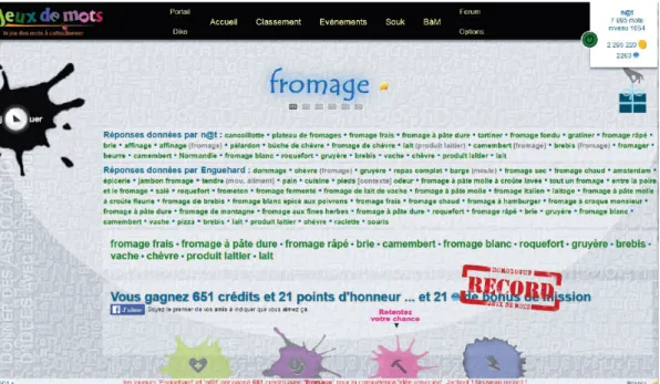
The quality and consistency of the relations are essential for a lexical network. Due to this fact, the validation of the relations which are anonymously given by a player is made also anonymously by other players. A relation is considered valid if it is given by at least one pair of players. A game happens between two players. A first player, let’s say player A, begins a game with prompting an instruction with a term T randomly picked from the database. The player A has then a limited time to answer which answer is applicable to the term T. The number of propositions which he can make is limited to letting the player not just type anything as fast as possible, but to have to choose the proper one. The same term with the same instruction is later proposed to another player B; the process is then identical. To increase the playful aspect, for any common answer in the propositions of both players, they receive a given number of points. At the end of a game, propositions made by the two players are shown, as well as the intersection between these terms and the number of points they win.

FIGURE 2.7: Screen-shot of an ongoing game with the target verb fromage (cheese) (taken form [Cha+17a]).

(43)

FIGURE2.8: Screen-shot of the game result with the target noun fro-mage (taken from [Cha+17a]).

Figure 2.7 shows a screen-shot of the user interface while figure 2.8 shows a pos-sible end of the game with the rewards. The figure illustrates answers of both players and the relevant scores.

(44)

Chapter 3 Modeling Meanings Preferences I:

Ranking Quantifier Scoping

3.1 Introduction

1

In this section, we start our preferential modeling on a particular linguistic phe-nomenon which is known as quantifier scoping.2 The focus is more on the question of how to rank the valid logical meanings of a given multiple-quantifier sentence only by considering the syntactic quantifier order. Thus, we do not take into account the other possible factors such as common sense and lexical knowledge, and we only work on different semantic ambiguities resulted from the quantifiers scoping in the logical formula as our meaning representations.

The problem of quantifier scope ambiguity has first appeared in [Cho65] in the following classical examples:

Example 3.1.

3.1a. Everyone in the room knows at least two languages.

∀x(Person(x) ∧ In_the_Room(x) → ∃y ∃z(Lang(y) ∧ Lang(z) ∧ y ≠ z ∧ Know(x, y) ∧ Know(x, z))

3.1b. At least two languages are known by everyone in the room.

∃y ∃z(Lang(y) ∧ Lang(z) ∧ y ≠ z ∧ ∀x(Person(x) ∧ In_the_Room(x) → (Know(x, y) ∧ Know(x, z)))

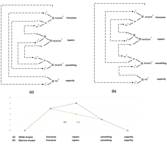
Chomsky argues that the order of "quantifiers" in surface structures plays a role in semantic interpretation. As it can be observed in the relevant logical formula of the examples 3.1a and 3.1b are not synonymous. We can give 3.1a the reading where each person may speak a different two languages and 3.1b the reading where the same two languages are spoken by everyone. These two readings differ only in the scopes of the quantifiers. In 3.1a, the existential quantifier is inside the scope of the universal quantifier. Thus 3.1a could be true in a room where everyone spoke differ-ent languages and 3.1b would be false in that room since the existdiffer-ential quantifier is outside the scope of the universal quantifier. Although, 3.1b would only be true in a room where everyone speaks the same two languages.

VanLehn [Van78] argues that the most accessible scoped reading for sentences with n quantifiers Q1 to Qn is the one where the scopes are in order of mention, 1_{The material in this chapter is derived in large part from [CM17] which is the author’s common} work with Davide Catta. The research in subsections 3.2, 3.3, partially 3.4.2, 3.5 and 3.6 are done by the author himself.

(45)

Ranking Quantifier Scoping

with Q1 widest and Qn narrowest. The main factor that may override this

prefer-ence is common-sense knowledge and this is something that we will not consider in our modeling in this chapter. The quantifier scope problem is not to describe all the factors which give these sentences their meanings. Because some of those factors involve discourse context and pragmatic knowledge and there is no precise formal-ization to capture those aspects.

Since sentences with quantifier scope ambiguities often have two (or more) non-equivalent semantic readings, capturing these phenomena with some plausible ranking techniques can potentially be useful for natural language inference systems. It is worth mentioning that different readings allow different inference paths and as it is shown in some studies that ([DGrt]) we can trace back the root cause of some invalid inferences in the misinterpretation of quantifiers as when occurs in quantifier scoping phase. Moreover, this kind of study is potentially suitable to be applied in some projects that gain meaning representations in logical forms from natural lan-guage texts by applying the Montagovian-style frameworks. One example of such project is e-fran AREN (ARgumentation Et Numerique) for the automated analy-sis of online debates by high-school pupils. The syntactic formalism that is used in the project is categorial grammars which are suitable for deriving meanings as the logical formulas. Grail [Moo17; Moo12], an automated theorem prover is used for parsing. It relies on a chart-based system close to categorial natural deduction which can rather smoothly be transformed to proof-nets.3

The problem of ranking the possible readings can be tackled if we employ the existing state-of-the-art techniques that use proof-nets for measuring the complexity of meaning representation [Mor00; Joh98]. We are specifically interested in Incom-plete Dependency Complexity Profiling introduced in [Mor00], but as we will see adopting this technique to our problem is not as straightforward as it seems. Our goal in this chapter is to fix these issues and extend Incomplete Dependency Com-plexity Profiling technique for the representing and ranking semantic ambiguities.4

The rest of the chapter is organized as follows: section 3.2 summarizes Gibson’s ideas on modeling the linguistic complexity of human sentence comprehension, namely IDT. In section 3.3, we recall the success and two limitations of IDT-based complexity profiling. In section 3.4, we define our new metric inspired by Hilbert’s epsilon and reordering cost. We show how it fixes some problems in previous work and how it gives a correct account of new phenomena. In section 3.5, we discuss some limitations that our approach has. In the last section, we conclude and we ex-plain possible future works.

3.2 Gibson’s Incomplete Dependency Theory

Incomplete dependency theory is based on the idea of missing incomplete depen-dency. This hypothesis can be explained during the incremental processing of a

3_{Two important features of the AREN project: (i) since the data are provided in written language by} the high-school pupils, we do not need to model intonation and prosody as a cue for disambiguation. (ii) there are, on average, 20 words in each sentence with almost two hundred category types, and the replies of the users happen with some delays. This restriction makes our solution scalable for this specific project that does not demand any big data analysis. Hence, it does not raise the issues of real-time processing and complexity.

4_{We will see in the chapter 6, how the introduced technique here can be combined with other} ap-proaches in linguistic complexity such as Distance Locality Complexity Profiling.

Modeling Preferences for Ambiguous Utterance Interpretations

HAL Id: tel-01908642

https://hal.archives-ouvertes.fr/tel-01908642v2

Interpretations

Mehdi Mirzapour

To cite this version:

THÈSE POUR OBTENIR LE GRADE DE DOCTEUR

DE L’UNIVERSITÉ DE MONTPELLIER

Présentée par Mehdi MIRZAPOUR

Le 28 septembre 2018

Sous la direction de Pr. Christian RETORÉ

et Dr. Jean-Philippe PROST

Modeling Preferences for

Declaration of Authorship

Abstract

Acknowledgements

Contents

List of Figures

List of Tables

List of Abbreviations

Chapter 1

Introduction

Chapter 2

Background Knowledge

2.1

Lambek Calculus

2.2

Categorial Proof Nets

2.3

Montagovian Generative Lexicon

2.4

JeuxdeMots : A Lexical-Semantic Network

Chapter 3

Modeling Meanings Preferences I:

Ranking Quantifier Scoping

3.1

Introduction

3.2

Gibson’s Incomplete Dependency Theory