HAL Id: hal-01394337
https://hal.archives-ouvertes.fr/hal-01394337
Submitted on 9 Nov 2016
HAL is a multi-disciplinary open access
archive for the deposit and dissemination of
sci-entific research documents, whether they are
pub-lished or not. The documents may come from
teaching and research institutions in France or
abroad, or from public or private research centers.
L’archive ouverte pluridisciplinaire HAL, est
destinée au dépôt et à la diffusion de documents
scientifiques de niveau recherche, publiés ou non,
émanant des établissements d’enseignement et de
recherche français ou étrangers, des laboratoires
publics ou privés.
A tutorial on the EM algorithm for Bayesian networks:
application to self-diagnosis of GPON-FTTH networks
Serge Romaric Tembo Mouafo, Sandrine Vaton, Jean-Luc Courant, Stephane
Gosselin
To cite this version:
Serge Romaric Tembo Mouafo, Sandrine Vaton, Jean-Luc Courant, Stephane Gosselin. A tutorial
on the EM algorithm for Bayesian networks: application to self-diagnosis of GPON-FTTH networks.
IWCMC 2016 : 12th International Wireless Communications & Mobile Computing Conference, Sep
2016, Paphos, Cyprus. pp.369 - 376, �10.1109/IWCMC.2016.7577086�. �hal-01394337�
A tutorial on the EM algorithm for Bayesian
networks: application to self-diagnosis of
GPON-FTTH networks
Serge Romaric Tembo
Orange Labs Lannion, France sergeromaric.tembomouafo @orange.com
Sandrine Vaton
T´el´ecom Bretagne Brest, France sandrine.vaton @telecom-bretagne.euJean-Luc Courant
Orange Labs Lannion, France jeanluc.courant @orange.comSt´ephane Gosselin
Orange Labs Lannion, France stephane.gosselin @orange.comAbstract—Network behavior modelling is a central issue for model-based approaches of self-diagnosis of telecommunication networks. There are two methods to build such models. The model can be built from expert knowledge acquired from network standards and/or the model can be learnt from data generated by network components by data mining algorithms. In a recent work, we proposed a model of architecture and fault propagation for the GPON-FTTH (Gigabit Passive Optical Network-Fiber To The Home) access network. This model is based on a Bayesian network which encodes expert knowledge. This includes depen-dencies that encode fault propagation and conditional probability distributions that encode the strength of those dependencies. In this paper we consider the problem of automatically tuning the above mentioned probability distributions. This is a parameter estimation problem under missing data conditions that we solve with the Expectation Maximization (EM) algorithm. Conditional probability distributions are learnt from the tremendous amount of alarms generated by an operating GPON-FTTH network during two months in 2015. Self-diagnosis is carried out to analyze the root cause of alarms. The performance of the diagnosis is evaluated with respect to an expert system based on deterministic decision rules currently used by the Internet Access Provider to diagnose network problems.
I. INTRODUCTION
Performing self-diagnosis of a telecommunication network with a model-based approach [1] [2] [3] [4] [5] [6] requires building an explicit representation of network architecture and behavior. Network architecture describes physical intercon-nections between components. Network behavior, also called fault propagation, describes how faults and alarms propagate through the distributed architecture. The consequence of both fault and alarm propagation is that a single root cause may result in a complex and distributed pattern of subsequent failures and their corresponding alarms [7].
There are two methods to model a telecommunication network for self-diagnosis. The model of network behavior can be built from some expert knowledge acquired from standards. The main difficulty encountered by experts is to keep the model close enough to the reality of the network while main-taining a high level of abstraction to make it independent with respect to the various engineering techniques implemented.
Another important issue is to model fault and alarm propa-gation through the distributed network. Fault propapropa-gation is a complex phenomenon because of the dynamic, distributed and non-deterministic behavior of telecommunication networks. A single fault may indeed generate multiple alarms, and a single alarm may be triggered by several faults.
In [8], we have proposed a model of fault propagation in GPON-FTTH (Gigabit Passive Optical Network-Fiber To The Home) access networks. This model is based on a Bayesian network [9]. Dependencies in the Bayesian network encode some expert knowledge acquired from ITU-T standards [10] [11]. A causal graph models the full chain of dependencies between faults or root causes, intermediate faults and the observed alarms. Probabilities quantify the strength of depen-dencies between nodes and their parents in the graph [12].
This Bayesian network model can be fine-tuned by mining data (faults and alarms) from operational GPON-FTTH access networks. Data may contain relevant knowledge that even a proven expert may not guess without the help of artificial in-telligence methods. Both the structure of the Bayesian network and its parameters, i.e. the conditional probabilities, can be fine-tuned with appropriate data mining algorithms [13] [14]. This article focuses on learning conditional probabilities that parameterize the Bayesian network by mining a database of alarms collected on a GPON-FTTH access network. It contains thousands of lines of alarms collected for example after calls of clients to the hot line of the access provider. In this context missing data occur because the root cause as well as some intermediate faults or alarms may not be monitored. To solve this problem we use the Expectation Maximization (EM) algorithm [15] and more particularly its adaptation to the case of Bayesian networks [16]. Our previously mentioned expert model of the GPON-FTTH network [8] is used as an initialization point for the EM algorithm.
We recall in Section 2 the basic concepts of paramet-ric estimation. Section 3 deals with Maximum Likelihood Estimation from incomplete data with the EM algorithm. EM for Bayesian networks is studied in Section 4. Section 5 demonstrates the application of the EM to fine tune the
probability distributions of the expert GPON-FTTH network model and assesses the performance of self-diagnosis with the Bayesian network model. Section 6 concludes and presents future works.
II. PARAMETER ESTIMATION WITHMLE A. Basic concepts on MLE
In statistics parameter estimation deals with estimating the value of parameters based on empirical data that has a random component.
As a matter of illustration let us consider a very sim-ple examsim-ple. Let us consider samsim-ples x1, x2, . . . , xT and
assume that these samples are independent and identically distributed realizations of a random variable X. X takes on the values {1, ..., K} with probabilities p1, p2, . . . , pK so that
P(X = i) = pi, ∀i ∈ {1, ..., K}. The problem of estimating
probabilities pi from measured/empirical data x1, x2, . . . , xT
is a problem of parameter estimation.
Maximum-likelihood estimation (MLE) is a particular method of estimating the parameters of a statistical model given data. MLE selects the set of values of the model parameters that maximizes the likelihood function. This is a way of finding out the set of values of model parameters for which observed data best ”fit” the model, in the sense that the likelihood of the empirical data is maximum.
We go back to our simple above mentioned example. The joint probability (or likelihood) of x1, x2, . . . , xT can be
factored into a product (because we assume that samples are independent) p(x1, x2, . . . , xT) = QTt=1p(xt) and the
log-likelihood can be factored as a sum L(x1, x2, . . . , xT) =
log p(x1, x2, . . . , xT) =P T
t=1log p(xt).
Each factor p(xt) equals one of the proportions pi
depend-ing on the value of xt i.e. p(xt) = P K
i=1pi1Ixt=i where 1I
is the indicator function (so that 1Ixt=i equals 1 if xt = i
and 0 otherwise). Equivalently, it holds that log p(xt) =
PK
i=11Ixt=ilog pi. All in all the log-likelihood equals:
L(x1, x2, . . . , xT) =Pt=1T PKi=11Ixt=ilog pi = PK i=1 PT t=11Ixt=ilog pi=P K i=1Nilog pi (1)
In the equation above Ni = P T
t=11Ixt=i is the number of
occurrences of the value i in the dataset x1, . . . , xT.
In this case MLE sums up to maximizing L(x1, x2, . . . , xT) =
PK
i=1Nilog pi with respect to the probabilities pi while
taking into account the normalization constraintPK
i=1pi= 1.
This constrained optimization problem can be solved with the lagrange multipliers method. Let us introduce Φ(p1, . . . , pK, λ) = P
K
i=1Nilog pi + λ(1 −P K
i=1pi). To
solve the problem, Φ should be maximized with respect to each pi and with respect to the lagrange multiplier λ. By
solving ∂p∂Φ
i = Ni
pi − λ = 0 one gets that pi is proportional
to Ni: pi= Nλi. And by solving ∂Φ∂λ = 1 −PKi=1pi= 0 one
gets λ =PK
j=1Nj = T so that pi= NiT .
In that very simple case of independent and identically distributed discrete valued samples the MLE is equal to the
set of empirical frequencies ˆpi = NTi i.e. the proportion of
samples that are equal to i. B. MLE for Bayesian networks
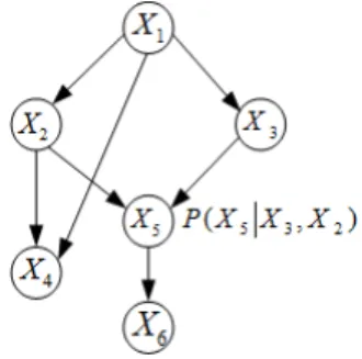
Let us now consider the problem of parameter estimation for Bayesian networks. A Bayesian network [9] (or probabilistic directed acyclic graphical model) represents a set of random variables and their conditional dependencies via a directed acyclic graph (DAG). See figure 1.
Fig. 1. A simple Bayesian network of 6 random variables.
In a Bayesian network (BN) nodes represent random ables and edges represent dependencies. These random vari-ables can be observations/measurements, latent varivari-ables or hypotheses for example. Each node is associated with a set of probability distributions that represent the distribution of the variable represented by the node, conditionally to the values of its parent nodes. These probabilities will be denoted as θi,j,k = P(Xi = k|pa(Xi) = j) where this quantity stands
for the probability that the value of node i is k given that the value of its set of parent nodes is j.
There are different definitions of what a BN is. Let X = (X1, X2, . . . , XN) be the set of nodes of the BN. One possible
definition is to state that the joint probability of nodes can be factored as the following product (or equivalently that the joint log-likelihood can be factored as a sum):
p(X; Θ) = QN
i=1P(Xi|pa(Xi)) =Q N
i=1θi,pa(Xi),Xi
L(X; Θ) = log p(X) =PN
i=1log θi,pa(Xi),Xi
(2) Here the notation p(X; Θ) (respectively L(X; Θ)) makes explicit that the joint likelihood (respectively log-likelihood) depends on the set of parameters Θ = (θi,j,k)i,j,k.
Let us now assume that several independent realizations (measurements) of the BN are available. Those measurements can be used in order to tune the set Θ of parameters so that the model fits the dataset (as much as possible). MLE of the probabilities θi,j,k can be performed from the measurements
X1, X2, . . . , XT. Note that each random variable Xtdenotes one realization of the BN, this realization being indexed by the upperscript t (1 ≤ t ≤ T ). Moreover each realization Xt = (X1t, X2t, . . . , XNt ) is a multivariate random variable where
the subscript i of Xit denotes node number i in the BN. The measurements dataset is denoted as D = (X1, X2, . . . , XT).
Because we consider independent successive realizations of the BN and because of the factorization of the joint probability
of nodes (Eq. 2) the log-likelihood of the dataset D can be splitted into a sum:
L(D; Θ) = T X t=1 L(Xt; Θ) = T X t=1 N X i=1 log θi,pa(Xt i),Xit (3)
We are now going to make explicit that this sum de-pends on the parameters θi,j,k by observing that many terms
are the same in the above sum. Indeed log θi,pa(Xt i),Xit =
P
j,k1Ipa(Xt
i)=j,Xit=klog θi,j,k and it is possible to merge the
equal terms:
L(D; Θ) =P
i,j,klog(θi,j,k)Ni,j,k (4)
where Ni,j,k =P T
t=11Ipa(Xt
i)=j,Xti=k counts the number of
records in the dataset D where the value of node Xi is k and
the set of values of its parent nodes pa(Xi) is j.
To maximize the likelihood of the dataset D it is then nec-essary to solve a series of constrained maximization problems:
maxP
klog(θi,j,k)Ni,j,k subject to Pkθi,j,k= 1 (5)
There are as many maximization problems as combinations of values for (i, j) and each optimization is performed with respect to the third subscript k of θi,j,k.
Each constrained maximization problem is similar to the problem solved in section II-A with a lagrange multiplier method. The result is then:
ˆ θi,j,k= Ni,j,k P kNi,j,k (6) which counts the empirical frequency of Xi = k when
pa(Xi) = j.
III. MLEFROM INCOMPLETE DATA WITH THEEM
ALGORITHM
A. Incomplete data
In statistics, missing data occur when no data value is stored for some variables in an observation. This can occur because measurements are not performed properly or because some variables are not reported. In BN some nodes are observa-tions/measurements whereas other nodes are hypotheses or latent variables. Latent variables (as well as hypotheses) are not directly observed but rather inferred from measurements. BN is consequently a setting in which incomplete data occur. MLE from incomplete data is not straightforward. Indeed most of the time it is not possible to compute the value of the likelihood of the dataset with incomplete data. Indeed let us assume that X is the vector of observed data (or measurements) and Y is a vector of missing data (or latent variables). Computing the joint likelihood p(X, Y ) of the complete data (X, Y ) is supposed to be straightforward under the considered model; this model can be for example a BN (in which case the expression of the likelihood is given by Eq. 2), or another parametric model that captures dependencies between random variables.
As Y is not measured it is unfortunately not possible to tune the parameters of the model by maximizing p(X, Y ; θ)
with respect to θ. Rather, the likelihood of observed data p(X; θ) should be maximized with respect to θ. But the computation of p(X; θ) is most of the time not tractable. Indeed p(X; θ) = P
Y p(X, Y ; θ) and the number of terms
in the sum P
Y is huge since this the product of the number
of states of each component of the vector Y . The complexity grows exponentially fast with the number of components in Y (e.g. number of nodes that represent a latent variable in the BN).
As the likelihood of the observed data p(X; θ) is not computationally tractable it is even more an issue to maximize p(X; θ) with respect to θ.
B. The Expectation Maximization (EM) algorithm
The problem of MLE from incomplete data can be solved with the EM algorithm [15]. As explained above computing the log-likelihood log p(X; θ) of the observed data is not possi-ble, whereas computing the log-likelihood of the complete data log p(X, Y ; θ) would be possible if only Y was not missing. It would then be possible to maximize log p(X, Y ; θ) with respect to θ.
As Y is missing, rather than maximimizing log p(X, Y ; θ) with respect to θ, the EM algorithm attempts to maximize iteratively the expected value of the log-likelihood of the complete data. Let us introduce Q(θ, θ0) as follows:
Q(θ, θ0) = E(L(X, Y ; θ)|X; θ0) (7) In the equation above E(•|X; θ0) stands for the expected value under the probability distribution of the missing data Y conditionally to the measurements X (for the value θ0 of the model parameters set).
EM is an iterative algorithm. At each iteration Q(θ, θr) =
E(L(X, Y ; θ)|X; θr) is maximized with respect to the first parameter θ, that is to say:
θr+1= Arg max
θ Q(θ, θ
r) (8)
Each iteration is decomposed into two steps: the expectation step (E step), and the maximization step (M step). The E step computes the probability distribution of missing data Y conditionally to the measurements X under the model with parameter θr(i.e. the current value of the parameter estimate). In practice this comes down to computing some statistics that summarize this conditional probability distribution, as it will be explained later in the particular case of the Bayesian network model. The E step is the most demanding step in the EM algorithm.
In the M step the function Q(θ, θr) is maximized with
respect to the first parameter θ so that an updated value θr+1
of the parameter estimate is obtained. Very often there exists a closed-form solution of this maximization problem so that the problem is simple to solve.
As stated before the EM algorithm is an iterative al-gorithm. It must be initialized with a value θ0. At each iteration the parameter estimate is updated as follows: at iteration 1, θ1 = Arg maxθQ(θ, θ0), then at iteration 2
θ2 = Arg max
converges to a stable value of θ. It has been proven that each iteration of EM increases the log-likelihood of measurement data, that is to say:
L(x; θr+1) ≥ L(x; θr). (9) As a consequence θr converges to a maximum of the
log-likelihood L(X; θ) of measurement data (or a saddle point). It is important to note that this maximum can be a local (but not necessarily global) maximum. In practice this means that the initial value θ0must be selected with care in order to avoid problems of convergenge to local (but not global) maximum.
IV. EMALGORITHM FORBAYESIANNETWORKS
A. M step
The EM algorithm has been adapted to the particular case of Bayesian networks [16]. In BN some nodes Xi may represent
variables that are missing. In this context the EM algorithm can be used to infer the probabilities θi,j,k= P(Xi= k|pa(Xi) =
j) from measurement data (that is to say from nodes which are not missing).
Recall from Eq. 4 that the log-likelihood has the following expression L(X; Θ) =P
i,j,klog(θi,j,k)Ni,j,kwhere Ni,j,k=
PT
t=11Ipa(Xt
i)=j,Xit=k.
Let us now make explicit that some nodes are measurements while other nodes are not observed (missing data). The former will be denoted as Xio,t while the latter will be denoted as Xim,t. Xio,tis the value of node Xi in the t-th observation of
the Bayesian network (t represents ”time”) and the upperscript o means that Xio,tis available (observed). Xim,tis the random variable associated to node Xi in the t-th observation of the
Bayesian network and the upperscript m means that Xim,t is missing (i.e. is not measured or the measurement value is not available).
As part of the nodes are not observed they are considered as random variables so that Ni,j,k = P
T
t=11Ipa(Xt
i)=j,Xit=k
is a random variable. The Q function of the EM algorithm introduced in Eq. 7 has the following expression:
Q(θ, θ0) =X
i,j,k
log(θi,j,k) ˆNi,j,k (10)
where Nˆi,j,k represent the expected count of number
of records where the value of node Xi is k and
the set of values of its parent nodes pa(Xi) is j:
ˆ Ni,j,k = E(P T t=11Ipa(Xt i)=j,Xti=k|X o, θ0). In this equation
Xo is the set of measurement data. As the expectation
E(•) is linear and as the expected value of the indicator function of a random event equals the probability of this event, it holds that Nˆi,j,k = P
T t=1γ t i,j,k where γt i,j,k = P(pa(X t
i) = j, Xit = k|Xo,t; θ0). This last quantity
represents the probability that Xit = k and pa(Xit) = j
conditionally to the measured nodes in the t-th observation of the Bayesian network.
The M step is the maximization of P
klog(θi,j,k) ˆNi,j,k
under constraint P
kθi,j,k = 1 for all values of (i, j). The
result of the M step updates the probabilities θi,j,kas follows:
θr+1i,j,k= ˆ Ni,j,k P kNˆi,j,k (11) B. E step
The E step computes, for each node Xi of the Bayesian
network, the conditional joint probabilities of Xi and its
parents γt
i,j,k = P(pa(Xit) = j, Xit = k|Xo,t; θr) as well as
the expected counts ˆNi,j,k=P T
t=1γi,j,kt . The computation of
the conditional joint probability γt
i,j,kis based on the algorithm
of propagation of evidence Xo,t on the junction tree [17] [18]
[19] representation of the Bayesian network. This inference algorithm allows us to run EM on the Bayesian network without worrying about loops. A potential is associated to each clique Cp and Cq of the junction tree and their common
separator Spq. A potential is a value associated to the random
variables belonging to a clique (or separator). The initial value of potentials is set as follows: φSpq = 1
φCp = QXi∈Cp,pa(Xi)⊂Cp∨pa(Xi)=∅P(Xi|pa(Xi); θ 0
) (12) where the product is taken over all the random variables Xi
that belong to the clique Cp and whose parents pa(Xi) also
belong to Cp (or do not have parents because they are root
nodes).
The algorithm of propagation of the evidence Xo,t on the junction tree updates the potential of all cliques Cp and Cq
and their common separator Spq. Assume the potential of a
clique Cp is already updated, i.e. the propagation of evidence
already reached the clique Cp but not yet the clique Cq. The
propagation algorithm proceeds as follows: the potential of the separator Spq is updated by marginalization, and then
the potential of the clique Cq is updated by applying a
multiplicative factor: φ∗ Spq = P Cp\Spqφ ∗ Cp φ∗ Cq = φCq φ∗Spq φSpq (13)
In the equation above the notation Cp\ Spq represents the
set of variables of the clique Cp which do not belong to the
separator Spq.
Propagation starts by recomputing the potentials of observed cliques., that is to say cliques where at least one random variable is observed. After that, updating operations are done in two recursive stages. The first stage (called collect) is performed by collecting evidence from leave cliques to root cliques. The second stage (called distribute) is performed by distributing evidence from root cliques to leave cliques.
At the end, the updated potential φ∗C
pof a clique Cpequals
the joint probability of evidence Xo,tand of random variables
belonging to clique Cp: φ∗Cp= P(Cp, X o,t; θr)
Note that for any family f = {Xi∪ pa(Xi)} of variables
the joint probability of the family f given measurement data Xo,t can be computed by marginalization:
γti,j,k= P(pa(Xit) = j, Xit= k|Xo,t; θ0) ∝ X
Cz\f
φ∗Cz (14)
where ∝ means ”proportional to” and the proportionality factor can be obtained by normalization.
V. APPLICATION OFEM ALGORITHM TOGPON-FTTH
ACCESS NETWORK
We applied in this section, the EM algorithm in order to learn the conditional probability distributions of the GPON-FTTH network model proposed in [8], based on a Bayesian network. Before doing this, we first talk about our motivations, i.e. the reason for which we need the EM algorithm.
A. Context
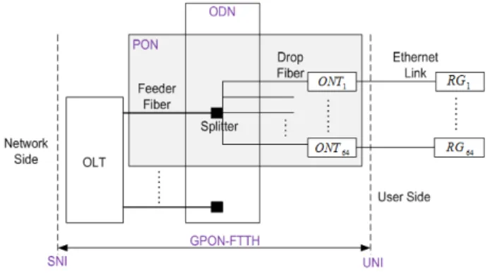
In [8], we proposed a model of the architecture and fault propagation of the GPON-FTTH access network [10] [11]. The GPON-FTTH network is made up of several PONs (Passive Optical Network). A PON has a tree-like topology which connects an Optical Line Terminal (OLT) with a maximum of 64 Optical Network Terminals (ONTs) in our example (see figure 2). Each ONT is connected to a RG (Residential Gateway) via an Ethernet link. A PON is a point-to-multipoint link through the ODN (Optical Distribution Network). The ODN can be decomposed into several splitting levels and each splitting level contains several splitters. Since there is no interaction between PONs, and all PONs have the same behavior, we have modeled one single PON. This model can be replicated to any PON of a GPON-FTTH access network.
Fig. 2. A simple engineering of the GPON-FTTH network
The model of the GPON-FTTH network proposed in [8] is a Bayesian Network (BN) which encodes expert knowl-edge acquired from ITU-T standards [10] [11]. The detailed description of nodes and dependencies of the GPON-FTTH model depicted by the figure 3 is given in [8]. From this expert knowledge we have built a causal graph of the full chain of dependencies between faults or root causes, intermediate faults and observed alarms. We have turned this graph into a Bayesian network by determining an order of magnitude
of conditional probabilities which quantify the strength of dependencies between nodes in the graph.
We have used this model to perform self-diagnosis of the GPON-FTTH network. In order to assess the performance of self-diagnosis with this BN model we have used two different approaches. A first approach described in [8] was to set up a physical testbed with a PON with two ONTs. Different faults were emulated, and alarms as well as counters were collected. The diagnosis of the root cause of alarms was performed with the BN approach. Seven usual fault scenarios were considered. Diagnosis results were inspected manually in order to assess their reliability. This demonstrated that self diagnosis based on a BN model was a reliable and promising approach.
In a second phase, a database of 10611 real diagnosis cases collected by Orange on a commercial GPON-FTTH network in july-august 2015 was analysed. Two tools have been compared: PANDA, the self-diagnosis tool based on the BN approach described in this paper, and DELC, a self-diagnosis tool based on deterministic decision rules. DELC is currently used to diagnose faults in the operational network. The different diagnosis were: no default (i.e. nominal GPON-FTTH network), faulty ONT, attenuating drop fiber, broken drop fiber, faulty or shutdown power supply, broken feeder fiber and unknown root cause. Over 10611 cases, DELC and PANDA took the same decision in 9768 cases (with 7393 cases of ”no default”). We analysed into details the cases where the diagnosis of DELC and PANDA were not the same. Interestingly, there were 766 cases out of 10611 where DELC was not able to produce a diagnosis whereas PANDA diagnosed most of the time that there was no default (716 cases) or located a particular default (50 cases: either faulty ONT, or attenuating drop fiber or power supply shutdown). DELC was not able to diagnose those cases because they were complicated and did not correspond to any of its decision rules. Maintaining a rule based decision system is a tedious task and it is almost impossible to take into account any possible combination of faults and alarms.
Nevertheless, we think that we can improve these self-diagnosis results if the parameters, i.e. the conditional proba-bility distributions of the GPON-FTTH model are fine tuned by a machine learning algorithm from the tremendous amount of data generated by the components of this network. The GPON-FTTH network data contain alarms, transmitted and received power of network components, transmission error counters, currents, voltages, temperatures and so on. Our dataset corresponds to two months of measurement on a commercial PON of the Orange FTTH access provider in july-august 2015. In pratice, there is always some situations where the network management system fails to get some values from some network components. These situations may be due for example to the filtering policy of network data applied by the network operator, or due to the communication loss between the network management system and one or many network components or due to some older devices that may not generate some facts. These situations lead to missing variables. That is why we have used the EM algorithm in order to
Fig. 3. The GPON-FTTH model based on Bayesian network.
automatically fine tune the expert parameters of the GPON-FTTH network model.
We have divided the dataset into two subsets. The first sub-set corresponds to 5130 diagnosis cases collected by Orange on a commercial GPON-FTTH network in july 2015. The second subset corresponds to 5481 diagnosis cases collected in august 2015. The first subset is the training dataset used to learn the parameters of the BN model with the EM. The second subset is the test dataset used to assess the performance of fault localization with the fine tuned BN model.
As explained in section III, the EM algorithm is initialized with a value θ0 of the parameters vector. In our case θ0
has been determined from operational expertise in diagnosing GPON-FTTH networks.
Figure 3 is a model of a PON of the GPON-FTTH network. A PON may contain up to 64 ON T s. All PONs have the same behaviour and there is no interaction between PONs. All ON T s also have the same behaviour. Therefore we have chosen to run the EM algorithm on a Bayesian network which models a PON containing only one ON T . The parameters of this ON T can be generalized to all ON T s connected to any PON. Note that if the GPON-FTTH changes, i.e. new nodes are added into the PON model, only the parameters of these new nodes and former nodes whose the parents set is updated, will be revaluated by the EM algorithm. We do not need to retrain completely the Bayesian network model.
B. Results of the application of EM algorithm for parameters learning of the GPON-FTTH network model
In this section, we assess the benefits of fine tuning the parameters by the EM, with respect to a diagnosis based on a
BN which parameters have been set by an expert. For doing so we compare the diagnosis results of PANDA over 5481 experimental cases in two situations: the model parameters have been set by an expert, or they have been moreover fine tuned with an EM by mining the whole dataset.
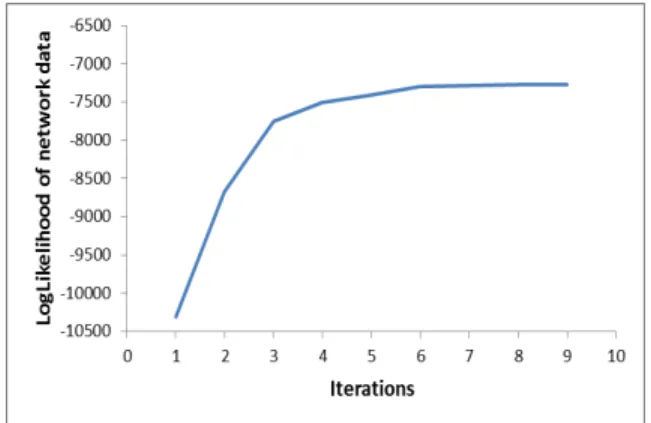
Figure 4 displays the evolution along the first iterations of the EM algorithm of the log-likelihood value of the 5130 real diagnosis cases collected by Orange in july 2015 on an opera-tional GPON-FTTH network. As stated by Equation 9 one can observe on Figure 4 that the log-likelihood of measurement data increases at each iteration of the EM algorithm. The log-likelihood stabilizes at a maximum value after 7 or 8 iterations, and the algorithm then converges.
Fig. 4. The Evolution of the Loglikelihood of network data with iterations.
From a practical point of view it is important to mention that we have encountered a few numerical problems with real measurement data. These problems appear when data do not
perfectly fit to the theoretical model (which bounds to happen when one deals with real data), for example if the dataset contains outliers. One problem that we have encountered concerns the update of some parameters by the M-step of the EM algorithm. In some cases it occurred that the value of a few expected counts ˆNi,j,k was equal to 0. This must be
interpretated as some combinations of events being considered by the E-step as absolutely impossible (taking into account measurement data). This causes numerical problems when one seeks to update the corresponding parameters by Equation [11] (divide by zero error). In those infrequent cases we have decided that the corresponding parameter should not be updated, that is to say that it is considered as a constant which is not estimated from data but set from expert knowledge. C. Diagnosis results
At that point we had two models: the expert model and the learned model. We have performed the diagnosis on the same cases separately with the two models. Table I shows a 2-dimensions confusion matrix which compares self-diagnosis results of the two models. The rows and columns of this matrix respectively represent self-diagnosis carried out with the expert model and with the learned model. Fine tuning the parameters of the model changed the diagnosis results in 185 cases out of the 5481 cases. This means that the order of magnitude of the parameters had been evaluated correctly by the expert. However it is interesting to analyze into more details cases where the diagnosis was different with a finely tuned BN, i.e. the cases corresponding to non-zero values outside the diagonal of the confusion matrix.
Each table from II to VI compares the two models for each instance of those cases (i.e. each non null element outside of the diagonal of the confusion matrix). The title of each of these tables is a short description of observations collected on the operating GPON-FTTH network for the considered case.
TABLE I
2-DIMENSIONSCONFUSIONMATRIX OF SELF-DIAGNOSIS RESULTS BETWEEN THE TWO MODELS.
Root causes 1 2 3 4 5 6 7 1 No Default 4030 0 0 7 6 0 9 2 Configuration Mistake 0 183 0 0 0 0 0 3 Faulty ONT 0 0 602 0 0 0 0 4 ONT power supply 0 0 0 402 0 0 0 5 Drop fiber attenuated 0 0 0 0 56 0 0 6 Drop fiber broken 0 0 0 0 14 0 0 7 Feeder fiber attenuated 0 0 149 0 0 0 32
Table II shows that, on a P ON of forty ON T s, when the upstream received power of an ON T denoted by ON T1is low
while the downstream received power of ON T1 is nominal,
the expert model does not detect any fault. This is a wrong diagnosis carried out by the expert model since the upstream optical channel between the OLT and ON T1is experiencing
attenuation. On the other hand, the learned model computes the appropriate diagnosis, i.e. attenuation of the drop fiber F iberDB1 of ON T1. Note that OK, AT and BR denote
TABLE II
PONWITH FORTYONTs. NO ALARM ON THEPON. UPSTREAM RECEIVED POWERRxOLT [1]OFON T1IS LOW. DOWNSTREAM RECEIVED POWER
RxON T [1]OFON T1IS NOMINAL. RECEIVED POWERS OF NEIGHBOR
ONTS ARE NOMINAL. Model Root causes States Beliefs
Expert F iberDB1 [OK, AT, BR] [0.9, 8.e-02, 3.e-06]
F iberDBi6=1 [OK, AT, BR] [0.9, 8.e-02, 3.e-06]
Learned F iberDB1 [OK, AT, BR] [9.e-02, 0.9, 2.e-06]
F iberDBi6=1 [OK, AT, BR] [0.9, 8.e-02, 3.e-06]
a fiber which does not attenuate, which attenuates or a broken fiber. This situation appears in 6 cases in the test dataset.
TABLE III
THEPONHAS FORTYONTs. NO ALARM IS OBSERVED ON THEPON. THE UPSTREAM AND DOWNSTREAM RECEIVED POWERSRxOLT [1]AND
RxON T [1]OFON T1ARE NOMINAL. THE RECEIVED POWERS OF NEIGHBORS OFON T1,I.E., RxOLT [i]ANDRxON T [i]FOR
i ∈ {2, ..., 40}ARE LOW. Model Root causes States Beliefs
Expert F iberDB1 [OK, AT, BR] [0.9, 8.e-02, 3.e-06]
F iberDBi6=1 [OK, AT, BR] [8.e-02, 0.9, 3.e-06]
F iberDB1 [OK, AT , BR] [0.9, 9.e-02, 2.e-06]
Learned F iberT [OK, AT, BR] [5.e-03, 0.99, 5.e-39]
F iberDBi6=1 [OK, AT, BR] [0.68, 0.31 , 0.001]
Table III shows a case for which the received power levels of ON T1are nominal while those of neighbors of ON T1are low.
In this situation the expert model diagnoses that the drop fiber of each neighbor of ON T1experiences attenuation. Doing so,
the expert model assumes that when the received power levels of at least one ON T on the PON are nominal, then the feeder fiber (denoted by F iberT ) shared by all ON T s connected on the PON cannot experience attenuation although the received power levels of other ON T s are low. This reasoning is not always true since for this diagnosis case it is the feeder fiber that attenuates. But this attenuation has not affected ON T1
since its received power levels were very high before the beginning of the feeder fiber attenuation. On the other hand, the received power levels of neighbors of ON T1were nominal
but very close to the lower bound of the range of nominal power values. We have observed 9 occurences of this case.
TABLE IV
PONWITH TWENTYONTs. NO ALARM ON THEPON. RECEIVED POWERS
RxOLT [i]ANDRxON T [i],FORi ∈ {1, ..., 20},ARE NOMINAL. TRANSMITTED POWERT xON T [1]OFON T1IS LOW. .
Model Root causes States Beliefs Expert AltON T1 [OK, ¬OK] [0.90, 0.10]
Learned AltON T1 [OK, ¬OK] [0.05, 0.95]
Table IV illustrates a case for which the learned model diagnoses that the power supply of ON T1 (denoted by
AltON T1) is faulty since the transmitted power level of this
ON T is low although all received power levels are nominal. On the contrary the expert model did not understand this strange situation and diagnosed that there was no default.
TABLE V
THEPONHAS FORTYONTs. ALARMSLOFus[1]ANDLOFds[1]ARE
OBSERVED FORON T1. THE UPSTREAM AND DOWNSTREAM RECEIVED POWERSRxOLT [1]ANDRxON T [1]OFON T1ARE MISSING. THE RECEIVED POWER LEVELS OF NEIGHBORS OFON T1ARE NOMINAL.
Model Root causes States Beliefs
Expert F iberDB1 [OK, AT , BR] [0.14, 0.34, 0.52]
F iberDBi6=1 [OK, AT, BR] [0.9, 8.e-02, 2.e-06]
Learned F iberDB1 [OK, AT, BR] [0.08, 0.86, 0.06]
F iberDBi6=1 [OK, AT, BR] [0.9, 8.e-02, 3.e-06]
Table V shows a situation for which LOF [1] (Loss of Frame) alarm is observed for ON T1and the received powers
of this ON T are missing. The expert model diagnoses that the drop fiber F iberDB1 of ON T1 is broken. This is wrong
since the loss of frames between OLT and ON T1 is not
due to the cut of the fiber but rather due to the poor quality of signal transmitted on this fiber, i.e, to fiber attenuation. The learned model performs an appropriate diagnosis. This situation occurred in 14 cases in the test dataset.
TABLE VI
THEPONHAS ONLY ONEONT. ALARMSLOSus[1]ANDLOSds[1]ARE
OBSERVED FORON T1. THE UPSTREAM AND DOWNSTREM RECEIVED POWERS, RxOLT [1]ANDRxON T [1]OFON T1ARE MISSING. Model Root causes States Beliefs
FaultyON T1 [+fto, ¬f to] [0.532, 0.468]
Expert F iberT [OK, AT, BR] [0.28, 0.43, 0.29] F iberDB1 [OK, AT , BR] [0.24, 0.35, 0.41]
FaultyON T1 [+fto, ¬f to] [0.960, 0.040]
Learned F iberDB1 [OK, AT , BR] [0.33, 0.36, 0.31]
F iberT [OK, AT , BR] [0.33, 0.34, 0.33]
Table VI shows a situation of communication loss between the OLT and the unique ON T connected to the considered PON. In this case, no information about neighbors of ON T1
help the expert model to discriminate between three root causes, feeder fiber attenuation (denoted by F iberT ), cut of the drop fiber or a faulty ON T1. The expert model does not
identify one root cause as being much more likely than the two others. The learned model diagnoses that ON T1 is faulty
but in practice it is impossible to decide this diagnosis is really more appropriate than the two other ones. We have observed this situation 149 times during our evaluation.
VI. CONCLUSION
We have studied into details the EM algorithm in the case of Bayesian networks. Basics of parameter estimation with a ML approach have been reminded. Then the EM algorithm has been described into details. It makes it possible to fine tune the parameters of a probabilistic model from incomplete data. The case of EM for Bayesian networks has been described, in particular evidence propagation over the junction tree representation that forms the E step.
This has been applied to faults self diagnosis in GPON-FTTH networks. We have analyzed a dataset of around 10000 diagnosis cases over a commercial network. 5000 cases, rep-resenting one month of data, have been used to fine tune
the parameters of the Bayesian network model with an EM algorithm. 5000 cases, representing the next month of data, have been used to diagnose faults. We have compared the diagnosis results when parameters have been set by an expert, and when they have been trained with an EM. The few cases where the diagnosis was not the same have been looked into details. The learned model reasonably improves self-diagnosis previously carried out by the expert model.
As future work we plan to automatically fine tune the graph of causal dependencies of the Bayesian network model i.e. learn or prune dependencies by mining real diagnosis cases.
REFERENCES
[1] B. Gruschke, “Integrated event management: Event correlation using dependency graphs,” in Ninth International Workshop on Distributed Systems: Operations and Management, 1998.
[2] S. K¨atker, “A modeling framework for integrated distributed systems fault management,” in IFIP/IEEE International Conference on Dis-tributed Platforms, 1995.
[3] K. Houck, S. Calo, and A. Finkel, “Towards a practical alarm correlation system,” in Fourth International Symposium on Integrated network management, 1995.
[4] J. F. Jordaan and M. E. Paterok, “Event correlation in heterogeneous networks using the OSI management framework,” in Third International Symposium on Integrated network management, 1993.
[5] S. K¨atker and K. Geihs, “A generic model for fault isolation in integrated management systems,” Journal of Network and Systems Management, vol. 5, no. 2, pp. 109–130, 1997.
[6] S. K¨atker and M. Paterok, “Fault isolation and event correlation for integrated fault management,” in Fifth international symposium on Integrated network management, 1997.
[7] C. Hounkonnou, Active self-diagnosis in telecommunication networks. PhD Thesis, European University of Brittany, University of Rennes 1, INRIA, ISTIC, France, 2013.
[8] S. R. Tembo, J. L. Courant, and S. Vaton, “A 3-layered self-reconfigurable generic model for self-diagnosis of telecommunication networks,” in IEEE SAI International Conference on Intelligent Systems, 2015.
[9] J. Pearl, “Bayesian networks: A model of self-activated memory for evidential reasoning,” in 7th Conference of the Cognitive Science Society, 1985.
[10] Telecommunication Standardization Sector of ITU, G.984.3 Recommen-dation. ITU-T, 2008.
[11] ——, G.977.1 Recommendation. ITU-T, 2003.
[12] J. Pearl, Probabilistic reasoning in intelligent systems: networks of plausible inference. Morgan Kaufmann, 1988.
[13] A. Cornu´ejols and L. Miclet, Apprentissage Artificiel, Concepts et Algorithmes. EYROLLES, 2013.
[14] F. V. Jensen and T. D. Nielsen, Bayesian Networks and Decision Graphs. Springer, Information Science & Statistics, 2007.
[15] A. P. Dempster, N. M. Laird, and D. B. Rubin, “Maximum likelihood from incomplete data via the EM algorithm,” Journal of the Royal Statistical Society, Series B, vol. 39, no. 1, pp. 1–38, 1977.
[16] S. L. Lauritzen, “The EM algorithm for graphical association models with missing data,” Computational Statistics and Data Analysis, vol. 19, pp. 191–201, 1995.
[17] S. Lauritzen, “Graphical models,” Oxford Statistical Science Series, Book 17, Clarendon Press, Oxford, 1996.
[18] A. L. Madsen and F. V. Jensen, “Lazy propagation: a junction tree inference algorithm based on lazy evaluation,” Artificial Intelligence, vol. 113, pp. 203–245, 1999.
[19] S. Lauritzen and D. Spiegelhalter, “Local computations with probabil-ities on graphical structures and their application to expert systems,” Journal of the Royal Statistical Society, Series B, vol. 50, no. 2, pp. 157–224, 1988.