Powder flow and mixing in a continuous mixer operating in either transitory or steady-state regimes: Mesoscopic Markov chain models

HAL Id: hal-02013428

https://hal-mines-albi.archives-ouvertes.fr/hal-02013428

Submitted on 10 Apr 2019

HAL is a multi-disciplinary open access

archive for the deposit and dissemination of

sci-entific research documents, whether they are

pub-lished or not. The documents may come from

teaching and research institutions in France or

abroad, or from public or private research centers.

L’archive ouverte pluridisciplinaire HAL, est

destinée au dépôt et à la diffusion de documents

scientifiques de niveau recherche, publiés ou non,

émanant des établissements d’enseignement et de

recherche français ou étrangers, des laboratoires

publics ou privés.

Powder flow and mixing in a continuous mixer operating

in either transitory or steady-state regimes: Mesoscopic

Markov chain models

Chawki Ammarcha, Cendrine Gatumel, Jean-Louis Dirion, Michel Cabassud,

V. Mizonov, Henri Berthiaux

To cite this version:

Chawki Ammarcha, Cendrine Gatumel, Jean-Louis Dirion, Michel Cabassud, V. Mizonov, et al..

Powder flow and mixing in a continuous mixer operating in either transitory or steady-state

regimes: Mesoscopic Markov chain models. Powder Technology, Elsevier, 2019, 346, pp.116-136.

�10.1016/j.powtec.2019.01.085�. �hal-02013428�

OATAO is an open access repository that collects the work of Toulouse

researchers and makes it freely available over the web where possible

Any correspondence concerning this service should be sent

to the repository administrator:

tech-oatao@listes-diff.inp-toulouse.fr

This is an author’s version published in:

http://oatao.univ-toulouse.fr/23675

To cite this version:

Ammarcha, Chawki and Gatumel, Cendrine and Dirion, Jean-Louis and Cabassud,

Michel

and Mizonov, Vadim and Berthiaux, Henri Powder flow and mixing in a

continuous mixer operating in either transitory or steady-state regimes: Mesoscopic

Markov chain models. (2019) Powder Technology, 346. 116-136. ISSN 0032-5910

Powder flow and mixing in a continuous mixer operating in either

transitory or steady-state regimes: Mesoscopic Markov chain models

Ammarcha C.

, Gatumel C.

, Dirion J.L.

, Cabassud M.

, Mizonov V.

, Berthiaux H.

⁎

c_{Department of Applied Mathematics, ISPEU, Rabfakovskaya 34, 153003 Ivanovo, Russia}

a b s t r a c t

a r t i c l e

i n f o

Continuous powder mixing is gaining interest in the industrial community concerned with more and more functional powder products. The understanding of powder flow and mixing/segregation of particles as well as their translation into models that can be used in process monitoring and control is a major issue. In the present work, we describe the development of different mesoscopic Markov chain models that are based on intercon-nected compartments or cells delimited in the mixing chamber. The general structure of the chain allows the der-ivation of either homogeneous or non-homogeneous markovian models, for which transition probabilities are state-dependent.

The models can be adapted to simulate variations of outflow rate, outlet mixture composition, hold-up weights and the distribution of these at the level of the compartments, during processing, including stationary and tran-sitory phases. This is applied to a Gericke 500 GCM® continuous mixer for either pure powders or their mixtures, in the latter case through the consideration of a Markov chain for each component. The models are fed by inde-pendent experiments that allow for the determination of the probabilities and the rules governing their change with the processing step, in particular during the transitory regimes. Agreement is found between model calcu-lation and experimental data for a wide range of configurations. The models can catch the variations of hold-up weights and internal or outlet flow rates at any rotational stirrer's speed during mixer start and steady state. They can reproduce the variations of the outflow rate, and therefore mixture composition, when dealing with a mixture of two components. This is also presented for two nominal compositions.

Conclusions are drawn in terms of process monitoring and control. It gives insights for process intensification, in particular for mixer design and the feeding configuration.

Keywords: Powder mixing Markov chain Continuous mixing Transitory regime 1. Introduction

Powder mixtures, or materials that once have been under the form of a powder mixture, are omnipresent in our everyday life. Metal alloys, cooking species, pharmaceutical pills or special concrete are current examples, and some can be made of up to twenty powder components depending on what the formulation stage has designed in terms of func-tionalities. Complexity of nowadays mixtures certainly lays in various factors, but can be wrapped by the idea that particles to mix are more and more of radically different rheological character, a statement that has been possible to make by the generalization of the FT-4 powder rhe-ometer in both academia and industry over the past years. But while this growing demand for more technological mixtures, targeting spe-cific properties at the consumer's scale, has been experienced during the last two decades, it has not been accompanied by a major

improvement from the part of the commercial mixing technologies themselves. Despite of the slow emergence of some more “chaotic” blenders, such as the Nautamixer® and the Turbula® mixer, the situa-tion depicted by Bridgwater at the beginning of the present decade [11] still holds true: mixing equipment in the industry are still the basic tumbler, ribbon or plough blenders, most of the time driven in the batch mode.

Continuous mixers can be seen as a viable alternative to face the challenges of today's functional mixtures:

- The increase of ingredients, which is cumbersome to handle for batch mixers to what concerns the order of introduction of the pow-ders, is just replaced by an increase of the number of Loss-In-Weight (LIW) feeders.

- Before entering the final continuous mixing step, ingredients can be premixed according to their rheological compatibilities or targeted functionalities. The premix can be performed either in continuous or batch, depending on the quantities involved.

⁎ _{Corresponding author.}

E-mail address:berthiau@mines-albi.fr(H. Berthiaux).

- On-line analysis of the quality attributes of the products or interme-diary has developed strongly over the past years and can be adapted to measure each of these functionalities in real-time.

- The operator-dependency, which is strong for batch processes, vanishes almost completely for continuous ones.

- Obviously, classical advantages hold true: reduced volume, simpli-fied scale-up and process validation, reduced waste and energy, easier link with yet continuous operations.

A good example of the batch to continuous dilemma for powders can be found in the pharmaceutical industry and is worth referring to. Anyone that has ever been concerned with powder mixing knows that the pharma industry can serve as the industry of reference because it is the only one that integrates standards on mixture homogeneity in its own norms and rules. Regulatory agencies such as the FDA in the US or the ANSM in France pushed the sector to develop the so-called Process Analytical Technologies (PAT) at the beginning of the 2000's in order to ensure the quality of the products (see [36]). Pharmaceutical firms had to develop ways of controlling “critical quality attributes” on-line, and in particular blend uniformity. This motivated analytical equipment ven-dors to adapt their equipment to the pharma environment and stimu-lated industry-academia collaborations, that in turn left footprints in the scientific literature of that period (see for example [15,30,53]). Fifteen years later, and as pointed out by Roche et al. [40] as well as Ierapetritou et al. [22], the FDA officially recommended the shift from batch to contin-uous processes. At that time, big pharma companies, such as Pfizer, BMS and Sanofi had already began their own transformation on a number of production lines. Today, companies of less international impact, such as Servier or Pierre Fabre in France are joining the movement.

In parallel to this industrial evolution, the understanding of continu-ous powder processing in general and continucontinu-ous mixing in particular from a chemical engineering standpoint has been the fact of very few re-search teams in the world and drew limited published works (see the paper by [34] on the situation at the time of their review). The following sub-areas of research on continuous powder mixers have been investigated:

- Definitions of mixture quality and mixer performance.

The definition of mixture's homogeneity requires first the determi-nation of a key component of the mixture: it can be the active pharma-ceutical ingredient, the bleaching agent, starch for icing sugar, etc. Homogeneity is then calculated (or estimated) by cutting the mixture into N portions (or considering n samples from the mixture) of size equal to that of the scale of scrutiny, to further derive the variance σ2

(or s2_{) of the compositions x}

iin the key ingredient. If μ (or xm) is the

mean content in key component in the mixture (or in the sampling set): μ¼1 N∑ N i¼1 ð Þxi σ2¼1 N∑ N i¼1 ð Þðxi−μÞ2 ð1Þ xm¼ 1 n Xn i¼1 xi s2¼ 1 n Xn i¼1 xi−xm ð Þ2 ð2Þ

Usually, the coefficient of variation, which is the ratio between the standard deviation and the mean, is better considered. It actually serves as a standard for pharma blend release on the market, as far as its value lies below 6%.

This set of definitions is well adapted for batch mixing because it re-flects the spatial distribution, and discrepancy in compositions, inside the equipment. But for continuous mixers, while the spatial distribution of the particles inside the mixer contributes to the building of a good mixture, it is not relevant to the definition of mixture homogeneity: only the outlet's mixture is of importance as it is the one that must pass quality controls. As a result, its variance calculation will be based

on the consideration of a set of N consecutive samples, a “window” of samples, taken at the outlet of the blender [18]. Therefore, Eqs.(1)– (2)are still holding true, but for a well-defined time period of produc-tion corresponding to that window of N samples.

Finally, and as pointed out by Weinekötter and Reh [51], a continu-ous mixer serves as a system able to reduce the spread in compositions between the inlet and the outlet of the equipment. Mixer performance is therefore evaluated by calculating the Variance Reduction Ratio (VRR), which is the ratio between the inlet variance and the outlet variance.

- Effects of operating variables at steady-state.

Most of the academic work done so far to what concerns continuous powder mixers concerns the effect of the operating variables on either the bulk particle flow or the mixture quality while the equipment is at steady-state. Marikh et al. [27] first investigated the effect of the rota-tional speed of the stirrer before publishing their work on the effect of the stirrer design on the hold-up weights and homogeneity of a com-mercial pharmaceutical mixture [29]. They emphasized the effect of the different flow regimes that can take place according to the choice of the operating variables. Effects of blade configuration, mass flow rates, and again stirrrer's rotational speed, have been reported over the same period of time for pharmaceutical systems by Prof Muzzio's team in New Jersey (see [33,38,49]). The work of Kingston and Heindel [24] on the effect on the rotation mode (co-rotating, counter-rotating, down or up-pumping) in a double-screw continuous mixer is also worth noting.

- Flow models and mixing models.

Modelling both the bulk particle flow and the blending of particles of different nature is undoubtedly the key in the understanding of contin-uous powder mixers. Kehlenbeck and Sommer [23] developed a two-dispersion coefficient (one for each component) model for a Gericke GCM 500 mixer. They identified the coefficients from the mathematical fitting of the results, which makes this model semi-empirical. Some years later, a Distinct Element Model (DEM) was being published by Sarkar and Wasgren [42] for spherical identical particles. This allowed the authors to derive local dispersion coefficients and define flow re-gimes according to a Froude number in a section of the mixer concerned with approximately 104_{particles. Although this is quite far from the real}

number of particles involved in an industrial mixer, for which wall ef-fects cannot be forgotten, this study caught some tendencies revealed earlier by Positron techniques [25] and shown that DEM can be employed as a building block for macroscopic models.

The need for a more global model, possibly able to include more microscopic thoughts, has then been the rule in modelling powder mixers. Sen et al. [43] and then Sen and Ramachandran [44] developed a Population Balance Model (PBM) to simulate data of Residence Time Distributions (RTD) obtained in Gericke GCM 250. The model formula-tion, although continuous in time and space, needs discretization and is finally close to a compartment model. The periodic section model de-veloped by Gao et al. [21] can be classified into this same category. These authors compared the model results with RTD data obtained numeri-cally and found good consistency. They emphasized the idea that their model do not include particle diversity and that segregation is still a challenge to account for in modelling. Another class of model uses the Markov chain approach and can be viewed as a generalization of com-partment models. As we will apply this modelling tool in the present work, the lector may refer to the specific section dedicated to it.

- Transitory operation and first process control strategies.

While a continuous mixer is aimed to operate at steady-state, transi-tory phases are taking place currently during normal production. First,

the equipment must start, which means that the hold-up weight will rise during a certain period of time before reaching a steady value, ac-cording to the operational conditions. Then, LIW feeders must be fed during processing which drives to strong perturbations because the vol-umetric mode of dosage is less accurate [10]. Finally, mixers must be emptied, again conducing to a transitory period for which process out-comes are decreasing and mixture quality is impacted. In previous works [1,2], we investigated the influence on hold-up weight and out-flow rates (still on the GCM 500) of various transitory phases, namely: emptying, starting and step-changes on the rotational speed N of the stirrer. We focused only on the bulk particle flow (no mixture) and de-rived empirical correlations through the frame of a single cell Markov chain model. Later on [3], we developed a system for on-line image analysis of simple mixtures, able to capture all the particles flowing out of the equipment and calculate mixture homogeneity in real-time. The influences of the scale of scrutiny, as well as that of N, on the quality of the mixtures were demonstrated. But the main outcome was that it was possible to evidence the extent of segregation in the mixer, as the mixtures produced during the starting phase were richer in coarse par-ticles (fines were accumulating in the equipment). This impacted clearly the quality of the mixtures when considering increasing step-perturbations on N, contrarily to negative steps.

The understanding and modelling of the transitory regime for a def-inite continuous mixer is also a prerequisite to monitoring and control of the operation, which can be viewed as the ultimate goal in the indus-trial implementation of such technologies. Published works by Ramachandran et al. [39], as well as Singh et al. [45] were concerned mostly by the compaction process, but gave general thoughts on the possible control strategies. From our side, we communicated on our first results on the regulation of the GCM 500 in the 2013 AIChE's annual meeting [54].

To sum up this small specific literature survey, it can be said first that it is far from being abundant, mainly the fact of 2–3 research teams in the world. One of the major ideas is that there is a fundamental need to explore what is going on inside continuous mixers and account for particle segregation. As we experienced ourselves, it seems that segre-gation “dictates” the bulk particle flow inside the mixer, and cannot be considered as an epiphenomenon. The parallel development of sys-temic/compartment models, that may in a second approach include DEM, to capture the process dynamics and be readily employed for pro-cess monitoring is also at stakes.

In the present work, we aim at developing and testing a mesoscopic model that accounts for the internal hold-ups and flow distributions in-side the GCM 500 mixer. The objective is to derive a tool that could sim-ulate and predict the behavior of the mixer in terms of outflow rates and mixture quality during both steady-state and transitory phases. For this, we will first focus on determining the distribution of the powder mass inside the mixer. This will then allow the determination of internal tran-sition probabilities to be integrated in a mesoscopic Markov chain model. Model testing and validation will be presented in terms of out-flow rate and mixture quality evolution during steady-state operation, as well as starting up and strong perturbations on the rotational speed of the stirrer.

2. Experimental set-up and methods 2.1. Mixer

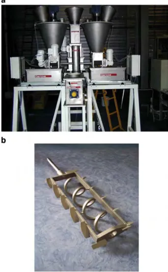
The mixing vessel studied in this work is the Gericke GCM 500 continuous mixer, equipped with two LIW feeders able to deliver a mass flow rate up to 50 kg h−1 _{each (see Fig. 1a). The}

hemi-cylindrical vessel is 50 cm long and 20 cm diameter. The mixing action is performed by a system of 10 blades mounted on a frame, whose axis is occupied by a screw-type shaft (Fig. 1b). The blades are ensur-ing a radial dispersion of the particles, while the screw is responsible for the axial movement of the bulk towards the outlet. Overall inlet

mass flow rate Qinas well as rotational stirrer speed N, are defining

the hold-up weight in the equipment. A too small ratio Qin/N will

drive to a nearly-complete emptying of the mixing chamber, while a too high ratio may lead to overflow and mixer shutdown. The range of rotational speed values is 10 to 50 Hz for a global mass flow rate that lies between 10 and 100 kg h−1

. In the present work, the inflow rate will be kept constant at 40 kg h−1_.

2.2. Particulate systems

Our goal is to gather the maximum information available so as to model the mixing process itself, letting the particulate system consid-ered as secondary. As in previous studies, we have chosen coarse and/ or fine couscous, depending on whether a “pure” product or a mixture of both is investigated. This system has the following advantages:

- Shape and density of the particles are identical, which leaves the par-ticle size as the sole difference, so as to give a clearer interpretation of the results.

- These products have experienced a cooking process, which confer them a certain time-stability.

- Products are cheap and easy to get hold of, which is important when high amounts of powders are to be handled.

- Mixtures can be analyzed easily through the image analysis method developed in earlier works.

- Mixtures can be separated by sieving and products can be re-used, as there is no overlap of the particle size distributions.

Fig. 1. Gericke GCM 500 facility showing the inlet chute, the mixing chamber, the LIW feeders (a); Stirring device used in this work (b).

Table 1gives the major physical characteristics of the products, in terms on both individual and collective properties. Both products are free-flowing as indicated by the Carr index. Fine couscous particles have been previously colored in black thanks to a process of iodine ad-sorption first described in Aoun-Habbache et al. [4]. This allowed a color contrast with the (white-yellow) coarse particles that could be detected by the image analysis system.

2.3. Determination of internal masses and flows

As stated, we need to access to the spatial-distribution and time-evolution of the hold-up weights and flow rates along the axis of the mixer, so as to implement these in a compartment-type markovian model. If we look at the blade configuration in the frame, it can be seen that opposite blades can be grouped two-by-two so as to define five compartments or cells, each comprised of two opposite blades. These cells are of equal volume.

Let Mi(t) be the powder mass in cell i at time t, M6(t) being the

cu-mulative mass measured at the outlet of the equipment. Mi(t) has

been measured experimentally by operating the mixer for the time t, stop it and then withdraw the whole powder mass corresponding to each cell by suction, beginning by cell n°5. This operation has been re-peated for up to 17 times in the time interval 0–150 s. Let Δt be a time interval (in the present work Δt will be chosen as Δt = 0.1 s). The net flowrate Qout, ileaving cell n°i between t and t + Δt reads:

Qout;i¼

P6

j¼iþ1#Mjðt þ ∆tÞ−Mjð Þt$

∆t ð3Þ

Therefore, internal flowrates between cells can be calculated by let-ting Δt be small enough to gain precision. In addition, if no back-mixing takes place in the mixer, the mean residence time in cell i can be derived as follows:

τið Þ ¼t

Mið Þt

Q_out;ið Þt ð4Þ

This procedure has been run for coarse couscous alone in the deter-mination of bulk flow characteristics, as well as for each product (coarse and fine couscous) in the determination of mixture flow characteristics.

2.4. Mixture composition analysis

Part of the presented work will deal with mixtures of fine and coarse couscous. The analysis of these will be performed on-line by an image analysis ring that has been fully presented in Ammarcha et al. [3]. A belt conveyor is placed at the mixer's outlet so as to form a single layer of particles by adjusting its speed to the inflow rate considered. A CCD linear camera placed perpendicularly to the belt captures all the particles passing under the camera and a specific routine created on Labview® allows the analysis of the images. Data treatment is per-formed through threshold procedures in order to detect fine couscous particles (white) from coarse couscous particles (black) and the con-veyor belt (green).

An image, which is the finest scale of scrutiny of the mixture that can be envisioned for our system, is defined by the accumulation of 200 consecutive single-pixel lines. Samples can be built by the grouping of various consecutive images, therefore defining various possible sam-ple masses. In the present work, we will consider the grouping of 21 consecutive images that correspond to a sample mass of 17.8 g of pow-der mixture. Results for two mixture compositions will be presented in the last section of this paper, namely a 50–50% by weight mixture and a 12.5–87.5% mixture of coarse and fine couscous respectively.

3. Mesoscopic Markov chain models developed 3.1. Some generalities

A Markov chain is a mathematical tool that has been employed to model countless systems in any field of science, such as the recognition of words in handwritten letters [14], direct marketing [35] or the previ-sion of significant weather events [41] to name a few.

In powder processes, it has been considered for several operations and equipment:

- Grinding: Wei et al. [52], Auer [5], Berthiaux [8], Catak et al. [12] - Filtration and sedimentation: Tory and Pickard [48], Nassar et al. [32] - Classification: Berthiaux and Dodds [7]

- Agglomeration: Catak et al. [13]

- Fluidized beds: Fan and Chang [19], Dehling et al. [16], Zhuang et al. [55]

- Rotating drums: Fan and Shin [20], Tjakra et al. [47]

- Mixing: Wang and Fan [50], Aoun-Habbache et al. [4], Ponomarev et al. [37], Legoix et al. [26], Balagurov et al. [6]

For more insights on the applications of Markov chains in particulate systems engineering, the reader can refer to the review paper by Berthiaux and Mizonov [9].

A Markov chain model aims at describing a systems' dynamics. First, this system must be decomposed into a finite number of inter-connected cells, also called “states”. The intensity of these connections, are quantified as transition probabilities between the states. Most of the time, the cells are corresponding to a distribution of the physical space that may advisably be based on physical thoughts or visual

Table 1

Main physical characteristics of the powders used. Particle size has been determined by sieving, true density by He pycnometer and apparent bulk densities by Erweka® “tap-tap” volumenometer. Carr and Hausner ratios are deduced from bulk densities.

Considered property Coarse couscous Fine couscous

d10(μm) 1375 680

d50(μm) 1700 860

d90(μm) 1970 980

(d90− d10)/2*d50 0.175 0.170

True density ρ (kg.m−3_{) 1452 1442}

Aerated apparent density ρa k(g.m−3) 762 759

Tapped apparent density ρt(kg.m−3) 779 787

Carr index: 100*(ρt− ρa)/ρt 2.22 3.60

Hausner ratio: ρt/ρa 1.02 1.04

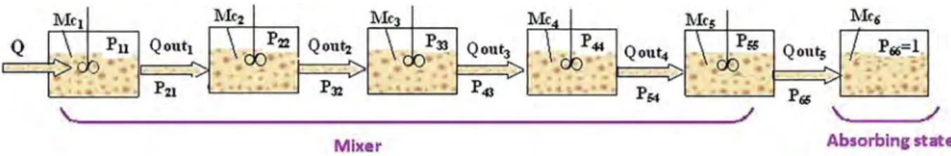
Fig. 3. General structure of the mesoscopic Markov chain representing the flow in the continuous mixer.

Fig. 4. Simulation of the evolution of the internal hold-ups and flowrates during the starting of a continuous mixer showing the influence of the recirculation ratio R. Qin= 40 kg h−1;

observations. In addition, transition probabilities are usually relative mass flows between cells that may adjust to mass balances.

Consider the simple case depicted inFig. 2that may represent the flow of powders in a certain equipment. It consists of four states, one of them being an absorbing state, which means that nothing can flow out of it. An absorbing state can therefore represent the outlet of a pro-cess. Let us observe the system after n transitions (or after any time rel-ative to a fix time interval) and be S(n) the state vector that represents the repartition of the powder in the four states Si(n) after those n tran-sitions (S(0) is the initial configuration):

S nð Þ ¼ S1ð Þn S2ð Þn S3ð Þn S4ð Þn 2 6 4 3 7 5 ð5Þ

Let pij(n) the transition probability, or the relative amount of powder

transiting from cell j to cell i during the nth transition, and P(n) the tran-sition matrix that gathers all the pij(n) values:

P nð Þ ¼ p₁₁ð Þn ⋯ p₁₄ð Þn ⋮ ⋱ ⋮ p₄₁ð Þn ⋯ p₄₄ð Þn 2 4 3 5 ð6Þ

In the present case:

p₄₁ð Þ ¼ pn 31ð Þ ¼ pn 42ð Þ ¼ pn 13ð Þ ¼ pn 14ð Þ ¼ pn 24ð Þ ¼ pn 34ð Þ ¼ 0 and pn 44ð Þ ¼ 1n

If S(n) and P(n) are known, S(n + 1) can be readily calculated by the recurring formula:

S n þ 1ð Þ ¼ P nð Þ S nð Þ ð7Þ

A Markov chain is said “homogeneous” when the transition proba-bilities are not varying with time or with the state of the system. In

this case Eq.(7)can be easily changed into:

S n þ 1ð Þ ¼ PnS 0ð Þ ð8Þ

If P is not constant, the chain is considered “non-homogeneous”, subcases being: linear chain if P depends only on n; non-linear chain if P depends both on n and S(n). Transition probabilities can change with time or with the state reached by the system in many cases involv-ing powders, as these can be compacted durinvolv-ing the mixinvolv-ing process or experience variation in the kinetics of grinding for a size reduction process.

3.2. General structure of the markovian models developed

To account for the horizontal configuration of the mixer and of the powder flow inside the vessel with the possibility of back-mixing, a gen-eral Markov chain that consists of n−1 cells allowing flows only be-tween contiguous cells can be envisioned (Fig. 3). As mentioned previously, the nth state is absorbing and figures out the outlet of the blender. The inlet is represented by an arrow to which is attached the inlet flowrate Qin. Let Mi(k) the powder mass in cell i and let Qij(k) be

the flow rate from cell j to cell i, after the kth_{transition. In the model,}

only flowrates between contiguous cells are allowed. The model's struc-ture lay between that of a full macroscopic black box model and that of a DEM model at the scale of a particle. It can be thought as a “mesoscopic model”.

If pij(k) is the transition probability for powders flowing from cell j to

cell i, and ΔF1(k) the powder mass introduced (at the inlet, cell 1) in the

mixer, the Markov chain can be established by the following rule:

M k þ 1ð Þ ¼ P kð Þ M k½ ð Þ þ ∆F1ð Þk&

M1ðk þ 1Þ M2ðk þ 1Þ ⋮ Mn−1ðk þ 1Þ Mnðk þ 1Þ 2 6 6 6 6 6 4 3 7 7 7 7 7 5 ¼ p₁₁ð Þk p21ð Þk 0 ⋮ 0 p12ð Þk p₂₂ð Þk p32ð Þk 0 … 0 p₂₃ð Þk p₃₃ð Þk p₃₃ð Þk … … ⋮ p_n−2;n−1ð Þk pn−1;n−1ð Þk pn;n−1ð Þk 0 0 ⋮ ⋮ pnnð Þk 2 6 6 6 6 6 6 4 3 7 7 7 7 7 7 5 ' M1ð Þ þ ∆Fk 1ð Þk M2ð Þk ⋮ Mn−1ð Þk Mnð Þk 2 6 6 6 6 6 4 3 7 7 7 7 7 5

The above set of notations allows for the possibility of feeding the equipment in cells other than cell 1, or distributing the feeding alongside the mixer. If Δt is the time interval through which the system is observed, assuming the inlet flow rate does not change with time, we also have:

ΔF1ð Þ ¼ Qk inΔt ð10Þ

Let αij(k) the ratio between the flowrates Qij(k) and Qin. We

basi-cally have:

Q_i−1;ið Þ ¼ αk i−1;ið Þ Qk inand Qiþ1;ið Þ ¼ αk iþ1;ið Þ Qk in ð11Þ

Let us consider cell 1. The probability p21(k) for a particle to transit

from cell 1 to cell 2 between the kth_{and the k + 1th state is the}

proba-bility (1 − p11(k)) to leave state 1 during this transition. The

corre-sponding mass leaving state 1 is therefore the product of (1 − p11(k))

by the mass present in state 1 after k transitions, which is M1(k) +

ΔF1(k). As this mass can only arrive in state 2 and is attached to the

flowrate Q21(k), we have the following equation:

1−p₁₁ð Þk

½ & M½ 1ð Þ þ ∆Fk 1ð Þk& ¼ Q21ð Þ∆tk ð12Þ

Replacing Q21(k) by Eq.(11)through Eq.(12)gives:

p₁₁ð Þ ¼ 1−αk 21ð Þμk 1ð Þ∆tk p21ð Þ ¼ αk 21ð Þμk 1ð Þ∆tk ð13Þ Where: μ1ð Þ ¼k Qin M1ð Þ þ ∆Fk 1ð Þk ð14Þ

A similar reasoning for the other cells drives to the following set of equations: p_iið Þ ¼ 1− αk i−1; ið Þ þ αk iþ1;ið Þk # $ μið Þ∆tk p_iþ1;ið Þ ¼ αk iþ1;ið Þμk ið Þ∆tk ð15Þ p_i−1;ið Þ ¼ αk i−1;ið Þμk ið Þ∆tk where: μið Þ ¼k Qin M_ið Þk ð16Þ

Eqs.(15)and(16)allow the construction of the transition matrix P(k) and the full description of the dynamics in transitory regime, if the initial state is known (usually empty cells). Eq.(16)also shows that transition probabilities not only depend on k (or time), but also on the previous state of the system (M(k)), which makes the general model non-homogeneous and non-linear.

When the mixer is at steady-state, all the back-mixing coefficients αi-1,Iare equals to a single value R, which may be dependent on

stirrer's design and rotational speed. The coefficients μiare also of

constant value, equal to μi, and can be seen as characteristic

frequen-cies or inverse of geometric residence times, each relative to cell i.

Therefore: R ¼ αi−1;I¼ αiþ1;I−1 μi¼ Q_in Mi and μ1 ¼ Qin M1þ ∆F1 ð17Þ

This time, the Markov chain is homogeneous and the steady-state transition matrix obtained is similar to that obtained by Tamir [46] for

a simpler case: P ¼ 1− 1 þ Rð Þμ1∆t 1 þ R ð Þμ1∆t 0 ⋮ 0 Rμ2∆t 1− 1 þ 2Rð Þμ2∆t 1 þ R ð Þμ2∆t 0 … … ⋮ Rμn−1∆t 1− 1 þ Rð Þμn−1∆t μn−1∆t 0 0 ⋮ 0 1 2 6 6 6 6 6 4 3 7 7 7 7 7 5 ð18Þ

Fig. 7. Distribution of the hold-up weights alongside the mixer for different rotational speeds of the stirrer, Qin= 40 kg h−1.

3.3. An example of simulation

The model presented above can be used to simulate any type of flow configuration and regime, such as starting-up, emptying, tracer pulse and Residence Time Distribution curves, inlet flowrate perturbations, staged feed, etc. To illustrate its potential, we will simulate the bulk powder flow inside the mixer during the start-up phase in terms of the distribution of the hold-up weights and the evolution of the internal flowrates.

As a first approach, we will consider the homogeneous matrix of Eq.(18)for a 6 cells case (5 mixer cells +1 absorbing) to perform the

simulations. This matrix only depends on the values of R and that of the μ_i, that are therefore necessary to run the model.

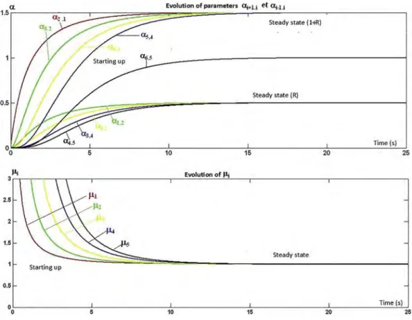
InFig. 4, we can see the simulation of the time-evolution of internal

hold-ups and flowrates during the start of the mixer, for two different values of R (0.5 and 10) and for μi¼ 1 s

−1

(whatever the cell i). The inlet flowrate is set at Qin= 40 kg h−1and the initial state vector is 0.

Afterwards, the masses in the states of the chain are calculated thanks to Eq.(9).

For R = 0.5, the hold-ups in the cells are higher in cell i than in cell i + 1, whatever the time considered. Steady-state is obviously reached earlier for the first cells of the mixer

Fig. 9. Evolution of the local net flowrates during the start of the mixer for different values of N, Qin= 40 kg h−1.

than for the last ones. After 15 s of simulation, all the internal masses are equal and steady-state is reached. The flowrates can be grouped according to their direction (forward for Qi+1,i

or backward for Qi,i+1). In each group, the flowrates

corre-sponding to the first cells are always greater than the following ones and they attain steady-state earlier. Forward flowrates reach a steady value of 60 kg h−1_{, while backward ones reach}

a 20 kg h−1 _{value, still in 15 s.}

As could be expected, a high recirculation ratio (R = 10) or back-mixing induces closer values for the hold-ups. The flowrates in the forward direction are also closer to each other, as well as those in the backward direction. The two types of flowrates are

Fig. 11. Recirculation coefficients R determined by the Levenberg-Marquardt algorithm through all the experimental data available, Qin= 40 kg h−1.

Fig. 12. Comparison of the homogeneous chain model's results with the experiments in terms of local outflow rates and internal hold-up weights during start-up, for various stirrer's rotational speeds, Qin= 40 kg h−1.

also closer to each other than for a much smaller recirculation ratio. Because of the high value of R, forward and backward steady-state flowrates are higher than the outlet flowrate Qout,

re-spectively 440 and 380 kg h−1_{. In addition, it seems that there is}

no influence of R on the attainment of the steady-state, which is reached after 15 s in all cases.

It is worth noting that, even if the transition matrix does not change with time because it has fixed values of R and μi, the

coeffi-cients αij(k) and μi(k) are changing during the transitory phase. For

instance, these are calculated at each step through:

μið Þ ¼k Qin M_ið Þk ;αiþ1;ið Þ ¼k Qiþ1;ið Þk Q_in and αi−1;ið Þ ¼k Qi−1;ið Þk Q_in:

Fig. 5shows the evolution these parameters during the simulation,

until they reach their steady values, respectively μi, 1 + R and R.

Being the mixer initially empty, the μi's are infinite for t = 0, then

de-crease towards μi. The flowrates coefficients are all starting from zero

Fig. 13. Simplified Markov chain non-homogeneous model.

Fig. 14. Evidence of a second-order relation between internal flowrates and hold-ups during the start of the mixer, driving to a linear relation for transition probabilities, Qin= 40 kg h−1,

(no initial flow) and increase towards their steady values, depending on whether they are concerned with forward flow or backward flow. The coefficient α6,5depicts the flow from the last cell to the outlet divided

by the steady outlet flow, its steady value is therefore equal to 1. This procedure can also be used to describe the process evolution during a step change in operating conditions, such as the stirrer's speed N. In

Fig. 6, internal hold-ups, as well as the outflow rate evolutions are

plot-ted after a step change from a value N1to a value N2, which may

corre-spond to the change from a matrix P1to a matrix P2. In this example, the

pair (R, μi) changes from (1, 0.2) to (10, 1). Because the mixer is already

at steady-state, the impact of the perturbation on the hold-ups is a global quick decrease of all the values to the new situation. The outflow rate experiences a strong perturbation through a peak that is close to 5 times Qin, before getting back to this nominal value. This is due to the

fact that R is instantly placed at a much higher value, which in turn forces particles to flow out of the equipment.

4. Single product bulk flow modelling 4.1. Internal hold-up weights and flow rates

The coarse product (coarse couscous) has been first investigated in terms of internal flows and mass distribution inside the blender.Fig. 7

shows the distribution of the hold-up weights measured experimen-tally in each of the 5 cells defined, for the flowrate Qin= 40 kg h−1

and rotational speeds varying between 10 and 40 Hz. Cells are experiencing a filling process one after another which is due to the chain construction. The masses in cells 1, 2, 3 and 4 follow identical trends, leading to a steady mass which is approximately the same whatever the cell.

In cell 5, which corresponds to the last mixing section before mixer's outlet, the powder mass is much higher, nearly five times that of the other cells. This is due to presence of the mixer's wall that corresponds

Fig. 15. Comparison of the non-linear chain model's results with the experiments in terms of local outflow rates and internal hold-up weights during start-up, for various stirrer's rotational speeds, Qin= 40 kg h−1.

to an outlet section which is much smaller than the section of the flow in the previous cells. More than half of the powder in the mixer is indeed in the last part of it, close to the outlet. The good mixing of this section is therefore critical.

For what concerns the impact of N, it can be seen that, at a fixed Qin,

the higher the speed, the smaller the hold-ups in every cells, which is not surprising. The steady-state values Miof the hold-ups can be plotted

against N (Fig. 8) and drive to the following empirical correlations after least square fitting of curves of the form Mi= ai/N + bi:

M_ið Þ ¼g 703

N for i ¼ 1 to 4 M5ð Þ ¼g 1714

N þ 60 ð19Þ

The data collected also allows for the determination of the local net flowrates in the forward direction ΔQi+1,iat any time and for each cell

by comparing the masses after a small time interval Δt: ∆Qiþ1;i¼ Qiþ1;i−Qi;iþ1¼

P6

j¼iþ1#Mjðt þ ∆tÞ−Mjð Þt$

∆t ð20Þ

The time evolution of these flowrates during the mixer's start is pre-sented inFig. 9. Each of these intermediary flowrates increases at a rate that is dependent on the rotational stirrer's speed N: as expected, higher

values of N drive to a quicker establishment of a steady-state. The steady value of the flowrates is the same whatever the cell considered, and is equal to the inflow rate Qin(which is 40 kg h−1in the present case).

Contrarily to what happens in the other cells, it can be noted that the outflow rate Q5,6, which is also that of the mixer Qout, only increases

after a minimal mass of approximately 40 g is attained in cell 5. This re-sult is emphasized inFig. 10, which represents ΔQi+1,ias a function of Mi

for cells 1 and 5, from which the following empirical correlation can be drawn and is valid during the transitory phase:

∆Qiþ1;ið Þ ¼ aMk 2ið Þ þ bMk ið Þ þ ck ð21Þ

Where a, b and c are parameters depending on N. 4.2. Homogeneous model

In this section, we will first consider the homogeneous model pre-sented above, which means that the transition matrix P is that of (Eq.(18)). P depends on six parameters, the five values of μiand R.

The μi’s are available from both Qinand the steady hold-up weight in

each cell i. As this is in turned linked to N through (Eq.(19)), we have a general relationship of μivs N. For the parameter R, we will proceed

Fig. 16. Comparison of the non-linear chain model's results with the experiments in terms of hold-up and outflow rate, during either a positive or a negative step perturbation of the stirrer's rotational speed (from 20 to 50 Hz and vice-versa), Qin= 30 kg h−1.

to an optimization scheme ruled by a Lenvenberg-Marquardt algorithm run on Matlab®, through minimalizing the following criteria D based on the internal hold-up weights:

D ¼X5 j¼1 X nexp i¼1 Mjð Þi # $ model− M# jð Þi$exp n o2 ð22Þ

In the above equation, nexp is the number of experimental data

considered.

This has been repeated for each rotational stirrer's speed and is plot-ted onFig. 11. As expected, R increases with N through what may be viewed as a power law, which is consistent with previous works on RTD in such mixers [28].

As explained in the example of simulation with this model, while the transition matrix does not vary with time, it can serve to calculate the evo-lution of the system during the transitory phases, such as the mixer's start through (Eq.(9)).Fig. 12shows the comparison of model and experi-ments in terms of internal hold-up weights Mi(t) (to which R has been

fitted) and local net flowrates ΔQi+1,i(t) which is derived from the Mi(t)’s.

Being the chain homogeneous, it is not surprising to see that the model results are all the more acceptable that the flow regime is at steady-state. Steady values of the flowrates and the hold-ups are well predicted by the model, whatever the rotational stirrer's speed is. While the model is still able to capture the global behaviors during the start of the mixer it fails in a fine description of the evolution of the hold-ups, in particular for cell 5. The outflow rate of the mixer ΔQ6,5is

also not well predicted. The model forces the particles to flow out of the equipment since the beginning of the run, while it has been recorded that a minimal mass Mmin,5in cell 5 was necessary for that to happen.

4.3. Non-homogeneous model

In the previous homogeneous model, the main difficulty came from the impossibility to measure or calculate all the flowrates Qi,j, but only net flow rates ΔQi+1,i. For this, we now consider a

simplified Markov chain model for which the exchanges between ad-jacent cells are replaced by these net flow rates. By doing so, we have: ΔQi+1,i= Qi+1,i.

This model (seeFig. 13) can be viewed as a series of continuous stirred tank reactors (CSTRs). The fact that no back-mixing is permit-ted is consistent with the data obtained on the hold-ups, the real mixing section being finally cell 5. As a result, the general matrix rule for the calculation of the internal hold-up weights, and subse-quent outflow rates, will be:

M1ðk þ 1Þ M2ðk þ 1Þ M3ðk þ 1Þ M4ðk þ 1Þ M5ðk þ 1Þ M6ðk þ 1Þ 2 6 6 6 6 6 4 3 7 7 7 7 7 5 ¼ p_1;1ð Þk p_2;1ð Þk 0 0 0 0 0 p_2;2ð Þk p_3;2ð Þk 0 0 0 0 0 p3;3ð Þk p_4;3ð Þk 0 0 0 0 0 p4;4ð Þk p5;4ð Þk 0 0 0 0 0 p5;5ð Þk p_6;5ð Þk 0 0 0 0 0 p6;6ð Þk 2 6 6 6 6 6 4 3 7 7 7 7 7 5 ( M1ð Þ þ ∆Fk 1ð Þk M2ð Þk M3ð Þk M4ð Þk M5ð Þk M6ð Þk 2 6 6 6 6 6 4 3 7 7 7 7 7 5 ð23Þ

As for (Eqs.(15)–(16)), the transition probabilities can be derived from the internal hold-up weights and flowrates:

p₂₁ð Þ ¼k Q21ð Þ∆tk M1ð Þ þ ∆Fk 1ð Þk p₁₁ð Þ ¼ 1−k Q21ð Þ∆tk M1ð Þ þ ∆Fk 1ð Þk for cell 1 p_iþ1;ið Þ ¼k Qiþ1;ið Þ∆tk Mið Þk p_iið Þ ¼ 1−k Qiþ1;ið Þ∆tk Mið Þk for cells 2 to 5 ð24Þ

InFig. 14, the flowrates Qij(k) measured inside the mixer are plotted

against the corresponding hold-up weights, for cells 1, 2 and 5, as well as for different values of N. Second-order correlations fits the data very well if the minimum mass Mmin,5is considered, which means that the

transition probabilities are following linear relationships with Mi(k):

i ¼ 1 : Q21ð Þ ¼ ak 1M1ð Þ Mkð 1ð Þ þ ∆Fk 1ð ÞkÞ; p21ð Þ ¼ ak 1M1ð Þ∆tk ð25Þ

i ¼ 2;3;4 : Qiþ1;ið Þ ¼ ak iMið Þk2;p_iþ1;ið Þ ¼ ak _iM_ið Þ∆tk ð26Þ i ¼ 5 : Q65ð Þ ¼ ak 5M5ð Þ Mk- 5ð Þ−Mk min;5.;p65ð Þ ¼ ak 5-M5ð Þ−Mk min;5.∆t

ð27Þ It must be noted that when M5(k) is smaller than Mmin,5, Q65= 0

and p65(k) = 0. TheFig. 14also shows the plots of pi+1,i(k) as a function

of Mi(k), confirming the above development.

The set of equations (Eqs.(25)–(27)) demonstrates that, as long as the internal hold-ups are evolving with time, such as during a transitory phase, the transition matrix depends on the actual state of the system. This means that the Markov chain is not only non-homogeneous, but also non-linear. When the hold-ups are steady, transition probabilities are all establishing themselves at a fixed value pij,max, for which internal

flowrates are replaced by Qin, the chain becoming then homogeneous:

p_21;max¼ Qin∆t M1þ Qin∆t p_iþ1;i;max¼Qin∆t Mi for cells 2 to 5 ð Þ ð28Þ

The maximum values of the probabilities can be extracted graphi-cally fromFig. 14, and used to determine the parameters ai:

a1¼ p_21;max M1 ai¼ p_iþ1;i;max Mi i ¼ 2;3;4 ð Þ a5¼ p_65;max M5−Mmin;5 ð29Þ If a new perturbation takes place, such as change in stirrer's rota-tional speed or mixer's emptying process, the hold-ups will change

towards their corresponding steady value. This will in turn affect the probabilities and the homogeneity of the Markov chain.

Fig. 15shows the results obtained by the new model, as compared

to the experimental results measured in terms of internal flowrates and hold-ups during the start of the mixer, for various rotational stirrer's speed. The model captures all these variations very well, in particular for the mixer's outflow rate that was not well predicted by the previous homogeneous chain. The small discrepancies that can be noted for N = 10 Hz can be attributed to the lack of stability of the speed itself.

To test the model a bit farther, negative and positive step perturba-tions on the stirrer's rotational speed have been imposed to the sys-tem after it has reached steady-state, both experimentally and numerically. The results are presented inFig. 16in terms of hold-up weights (within cells or global) and outflow rate of the mixer. The model proves here that it follows extremely well the strong perturba-tions during its occurrence, as well as it succeeds in predicting the new stable regime.

5. Binary mixture flow modelling 5.1. Derivation of a non-homogeneous model

To model the flow of a binary mixture that consists of coarse and fine particles, we will consider that each type of particle is following a Markov chain on its own. We therefore have two transition matrices Pc(k) and Pf(k) that correspond to the coarse particles and the

fine particles respectively, made of transition probabilities pcij(k) and

pfij(k), but also states vectors Mc(k) and Mf(k), each consisting of the

masses Mci(k) and Mfi(k) in the 6 cells defined above, as well as inlet

masses ΔFc(k) and ΔFf(k). After k transitions, the particle flow is

Fig. 18. (a) Evidence of the equality of the minimal masses in cell 5 (a); (b) fine particles content of the minimal mass in cell 5 according the various operational conditions considered (b), Qin= 40 kg h−1.

Fig. 19. Simulation of mixer start, mixture 1, two different values of N - (a) Comparison of the Markov chain model's results with the experiments in terms of outflow composition; (b) p65–

therefore ruled by the following equations: Mc1ðk þ 1Þ Mc2ðk þ 1Þ Mc3ðk þ 1Þ Mc4ðk þ 1Þ Mc5ðk þ 1Þ Mc6ðk þ 1Þ 2 6 6 6 6 6 6 6 6 4 3 7 7 7 7 7 7 7 7 5 ¼ p_c1;1ð Þk p_c2;1ð Þk 0 0 0 0 0 p_c2;2ð Þk p_c3;2ð Þk 0 0 0 0 0 p_c3;3ð Þk p_c4;3ð Þk 0 0 0 0 0 pc4;4ð Þk p_c5;4ð Þk 0 0 0 0 0 p_c5;5ð Þk p_c6;5ð Þk 0 0 0 0 0 p_c6;6ð Þk 2 6 6 6 6 6 6 6 6 4 3 7 7 7 7 7 7 7 7 5 ( Mc1ð Þ þ ∆Fk c1ð Þk Mc2ð Þk Mc3ð Þk Mc4ð Þk Mc5ð Þk Mc6ð Þk 2 6 6 6 6 6 6 6 6 4 3 7 7 7 7 7 7 7 7 5 Mf 1ðk þ 1Þ Mf 2ðk þ 1Þ Mf 3ðk þ 1Þ Mf 4ðk þ 1Þ Mf 5ðk þ 1Þ Mf 6ðk þ 1Þ 2 6 6 6 6 6 6 6 6 6 4 3 7 7 7 7 7 7 7 7 7 5 ¼ pf 1;1ð Þk pf 2;1ð Þk 0 0 0 0 0 p_{f 2;2}ð Þk p_{f 3;2}ð Þk 0 0 0 0 0 p_{f 3;3}ð Þk p_{f 4;3}ð Þk 0 0 0 0 0 p_{f 4;4}ð Þk pf 5;4ð Þk 0 0 0 0 0 p_{f 5;5}ð Þk p_{f 6;5}ð Þk 0 0 0 0 0 p_{f 6;6}ð Þk 2 6 6 6 6 6 6 6 6 4 3 7 7 7 7 7 7 7 7 5 ( Mf₁ð Þ þ ∆Fk f 1ð Þk Mf 2ð Þk Mf 3ð Þk Mf 4ð Þk M_{f 5}ð Þk Mf 6ð Þk 2 6 6 6 6 6 6 6 6 6 4 3 7 7 7 7 7 7 7 7 7 5

Obviously, the hold-up weight Mi(k) and the composition Xfi(k) in

fine particles in cell i are given by: Mið Þ ¼ Mk cið Þ þ Mk fið Þk Xfið Þ ¼k

Mfið Þk

Mcið Þ þ Mk fið Þk

ð32Þ

In particular, the outlet composition of the mixture can be calculated through (note Q_fijand Qmijare the local net flow rates in fine and coarse

particles respectively): Xfð Þ ¼k Qf 65ð Þk Qc65ð Þ þ Qk f 65ð Þk ¼ pf 6;5ð ÞMk f 5ð Þk p_{f 6;5}ð ÞMk f 5ð Þ þ pk c6;5ð ÞMk c5ð Þk ð33Þ Xcð Þ ¼k Qc65ð Þk Q_c65ð Þ þ Qk f 65ð Þk ¼ pc6;5ð ÞMk c5ð Þk p_{f 6;5}ð ÞMk f 5ð Þ þ pk c6;5ð ÞMk c5ð Þk ð34Þ

Because the same equations hold for either the coarse or the fine particles, we will limit our analysis to the fine product.

As for the bulk flow model, the transition probabilities are linked to the flow and masses through:

pf 21ð Þ ¼k

Qf21ð Þ∆tk Mf1ð Þ þ ∆Ffk 1ð Þk

for cell 1; pfiþ1;ið Þ ¼k

Qfiþ1;ið Þ∆tk Mfið Þk

for cells 2 to 5

ð35Þ When steady-state is reached, probabilities are assigned to their steady values. So if Mf_iis the steady hold-up in cell i, those maximum probabilities are: p_{f 21} / 0 max¼ Qf_in∆t Mf₁þ Qfin∆t p_fiþ1;i / 0 max¼ Qf_in∆t Mf_i for cells 2 to 5 ð36Þ We further assume a linear relationship between the probabilities and hold-ups by the introduction of constants afithat can be linked to

the steady-state probabilities:

pfiþ1;ið Þ ¼ ak fiMfið Þk for cells 1 to 4

pf 6;5ð Þ ¼ ak f 5Mf5ð Þ−Mfk min;5ð Þk # $ for cell 5 ð37Þ af 1¼ Qf_in∆t Mf₁ Mf₁þ Qfin∆t h i afi¼ Qf_in∆t Mf_i2 a_{f 5}¼ Qfin∆t Mf₅ Mf₅−Mfmin;5ð Þk h i

Fig. 20. Simulation of mixer start, mixture 2, two different values of N - Comparison of the Markov chain model's results with the experiments in terms of outflow composition, Qin=

The last step is to transform these equations into a probability-based set of equations that demonstrates the homogeneous and non-linear character of the Markov chain:

p_{f 21}ð Þ ¼k Mf1ð ÞQfk in∆t Mf₁ Mf₁þ Qfin∆t h i p_fiþ1;ið Þ ¼k Mfið ÞQfk in∆t Mfi 2 ð38Þ p_{f 65}ð Þ ¼k Mf5ð Þ−M fk min;5 # $Qf_in∆t Mf₅ Mf₅−M fmin;5 h i

5.2. Internal hold-up weights

For the matrix calculation of the states to be performed, the knowl-edge of the steady-state values of the internal hold-ups, as well as that of the minimal mass in cell 5 must be known. For this, experiments of de-termination of internal hold-up weights have been performed for each product during their mixing, as described earlier for the single product. The content of each cell has been withdrawn from the blender at differ-ent momdiffer-ents of time and sieved so as to separate coarse and fine cous-cous, afterward each product could be weighed. This procedure has been repeated until the steady-state regime has been reached. Two cases have been investigated, namely a 50–50% by weight mixture and a 87.5 coarse - 12.5 fine % by weight mixture. These two mixtures will further be identified by mixture 1 and mixture 2 respectively.

Fig. 17shows the fine particle content in the five cells at steady-state

for the two mixtures. As commented in Ammarcha et al. [3], the first four cells are richer in fine particles than the last cell, whatever the con-ditions under which the blender operates, pointing out the presence of a segregation effect. As for the coarse product alone, it can be shown that the steady hold-up weight of the mixture in each cell can be assimilated to that of coarse couscous, which means that (Eq.(19)) holds true. This allows for the determination of the steady hold-up weights of each com-ponent in every cell Mf_iand Mccithrough the empirical relations:

Mf_i¼ Xfi( 703 N ð Þ;g Mci¼ 1−Xfi -. (703 N ð Þ for i ¼ 1 to 4g ð39Þ Mf₅¼ Xf 5( 1714 N þ 60 3 4 g ð Þ;Mc5¼ 1−Xf 5 -. ( 1714 N þ 60 3 4 g ð Þ ð40Þ

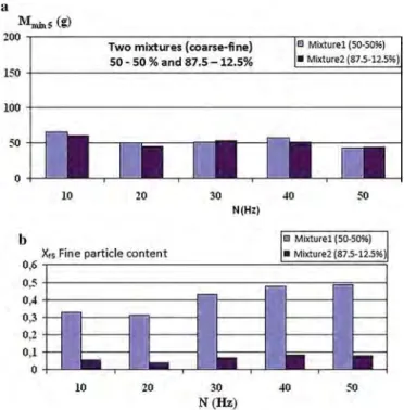
The minimal mass of each product has been also determined exper-imentally by stopping the mixer when the first particles begin to flow out of it, withdrawing the content of cell 5, sieve it and weigh the sepa-rated components.Fig. 18a shows that the overall minimal mass in cell 5 can be assumed to be a constant equal to 50 g, whileFig. 18b shows that the content in fine particles depends on N, in particular for mixture 1. As expected, a higher value of N drives to a mixture that is closer to the nominal value of 50% by weight for this mixture. For mixture 2, a segre-gated mixture is still present in the last cell, but its composition will change as steady-state is approached.

5.3. Binary mixing model validation

The validation of the model has been performed by comparing its re-sults in terms of outlet's mixture composition to the measurements that have been obtained through on-line image analysis. This evaluation is based on two process operations: the start of the blender towards the attainment of steady-state and negative/positive step perturbations on the stirrer's rotational speed.

Fig. 19a presents model and experimental results obtained during

the starting phase of the equipment for two stirrer's rotational speeds, for mixture 1. In both cases, the model catches the evolution of the com-position very well. In particular, it predicts the fact that the mixture is richer in coarse particles during the start of the mixer, a segregation phenomenon we discussed in a recent work [3].Fig. 19b shows the lin-ear relationships between the evolving probabilities and the hold-up weights for cell 5 and for both component. As commented before, the probabilities are increasing with the hold-up until they reach their steady value, afterwards the calculation rule become that of an homoge-neous chain. In addition, it can be seen that the minimum mass of pow-der that allows the outflow of the mixture, and can be estimated by adding the hold-up weights in cell 5 for each component, is roughly the same whatever the stirrer's speed and equal to 50 g. Finally, and as expected, the higher the stirrer's speed, the higher the probability for the particles to get out of the equipment. Results corresponding to mixture 2 are presented inFig. 20. Once again, the model reproduces the experiment quite well but is unable to catch the small-scale mass fluctuations that have been recorded for each component.

Fig. 21. Simulation of negative and positive perturbation steps, mixture 1 - (a) Comparison of the Markov chain model's results with the experiments in terms of outflow composition; (b) p65–M5probability plots, Qin= 40 kg h−1, Δt = 0,1 s.

A negative step perturbation on the rotational speed (from 50 to 10 Hz) has been imposed to the system operating with mixture 1 and is depicted inFig. 21a. In this graph, both coarse and fine products are represented. In the same figure, the results for a

positive step perturbation (from 25 Hz to 45 Hz) are shown. What-ever the case, the model is adequate in representing the evolution of the composition during the perturbation, in particular the way the system is able to reach another steady-state configuration.

The evolution of the transition probabilities during the whole pro-cess is presented inFig. 21b, only for cell 5. In the case of the neg-ative step, the probability increases with the local hold-up until it reaches the maximum value that corresponds to steady-state. At the time of the perturbation, this operating point is no longer valid. The system therefore has to catch the p65–M5line that

cor-responds to the operation under the new condition (10 Hz), after-wards the probability will evolve until it reaches the corresponding maximum value (approximately 0,006 for coarse particles). This is exactly the same that happens for the positive step (Fig. 21c), with the exception that at the moment of the perturbation, the probability that corresponds to the same hold-up – but for the higher stirrer's speed- is much higher (nearly 0,023) than the max-imum probability under this operating condition (0,013). The path followed to reach this steady value is in fact the extension of the p65 – M5 line that can be drawn in a mixer start experiment

under the condition N = 45 Hz. Results relative to mixture 2 are presented inFig. 22. They are globally similar to those obtained with mixture 1. However, it can be seen that the model fails in de-scribing finely what happens during the two types of perturbation, in particular it predicts that the system will join steady-state earlier than in reality. Once again, the fluctuations that are appearing can-not be caught by the Markov chain in its present form. Various thoughts, underlining some of the model limitations, can be brought to partially explain this:

- The transition probabilities are defined for each component in-dependently of the other, at the scale of the cells. Mixture 2, being mostly composed of coarse particles, could be more sensi-ble to this hypothesis as the fine particles flow could be affected by the presence of the coarse particles. An improvement of the model would therefore be, for each component, to account for the presence of the other component in the transition matrix, for example by including a function of the composition directly in the probabilities.

- The time interval Δt chosen for the simulation is fixed and equal to 0.1 s. For a typical flow rate of 40 kh.h−1_{, this corresponds to}

1 g, or roughly to 500 couscous particles. There is therefore a lim-itation to the use of equations(39)and(40)as they put together mass values that may correspond to 1000 times the particles in-volved in Δt.

- The mixture is dumped from the outlet mixer's gate onto the belt and conveyed through the image capture systems. There may be some segregation at the outlet gate or on the, belt causing the variations in compositions that are experienced.

6. Concluding remarks

The Markov chain models developed in this work have proven their efficiency to catch the major process changes in terms of mass flows, mixture composition and hold-ups, for a wide range of typical process situations such as: mixer start, mixer stop, negative or positive steps on the rotational speed. They do not seem able to figure out the extent of the small-scale fluctuations on the composition of the mixtures that are recorded at the outlet of the equipment, especially for mixture 2 which is mainly composed of coarse particles by weight. It is unclear to what phenomena or factor this may be attributed.

Markov chains also need experimental input to calculate the transi-tion probabilities, even if it can be done through various independent experiments. There is indeed a great interest, in process monitoring as well as in process development, in trying to link this input to the output of a DEM modelling scheme, so as to derive a hybrid model catching the whole system at any scale. Such models have emerged some ten years ago (see [17]) and are still looking very promising, although they need to be properly implemented to include the complexity of the particulate system and that of the mixer itself.

The intensification of the mixing process is also worth investigating. For instance, there is a lot work to undertake in terms of stirrer design so as to induce perfect mixing in a horizontal configuration that is much proper to plug flow. The same holds true for the LIW feeders for which the smoothing of the mass flow fluctuations due to the feeding screw is a key issue. The location of these feeders along the mixer needs to be studied into details because, as we pointed out in the pres-ent work, segregation by percolation takes place close to the inlet wall. This means that it may advisable to consider other feeding configura-tions, such as placing the segregating component's feeder to another place, and even so distributing the feed over the mixer's length. This has been theoretically considered by Mizonov et al. [31], again through a Markov chain model, but needs to be experimentally studied.

The immediate following step for this research work is to implement a process control loop, transforming the outlet mixture homogeneity signal into an action on the rotational stirrer's speed. This will help smoothing the fluctuations that appear during transitory phases or when LIW feeders are operating in the volumetric mode, like for hopper re-filling. This will be discussed in further papers.

References

[1] C. Ammarcha, C. Gatumel, J.L. Dirion, M. Cabassud, H. Berthiaux, Predicting the con-tinuous powder mixing dynamics in transitory regimes, Adv. Powder Technol. 23 (2012) 787–800.

Fig. 22. Simulation of negative and positive perturbation steps, mixture 2 - Comparison of the Markov chain model's results with the experiments in terms of outflow composition, Qin=

[2]C. Ammarcha, C. Gatumel, J.L. Dirion, M. Cabassud, V. Mizonov, H. Berthiaux, Transi-tory powder flow dynamics during emptying of a continuous mixer, Chem. Eng. Process. Process Intensif. 65 (2013) 68–75.

[3]C. Ammarcha, C. Gatumel, J.L. Dirion, M. Cabassud, H. Berthiaux, Continuous powder mixing of segregating mixtures under steady and unsteady state regimes: homoge-neity assessment by real-time on-line image analysis, Powder Technol. 315 (2017) 39–52.

[4] M. Aoun-Habbache, H. Berthiaux, M. Aoun, V. Mizonov, An experimental method and a Markov chain model to describe axial and radial mixing in a hoop mixer, Pow-der Technol. 128 (2–3) (2002) 159–167.

[5] A. Auer, Das probabilitische modell des kontnuierlichen zerkleinern, Powder Technol. 28 (1981) 77–82.

[6]I. Balagurov, V. Mizonov, H. Berthiaux, C.A. Gatumel, Markov chain model of mixing kinetics for ternary mixtures of dissimilar particulate solids, Particuology 31 (2017) 80–96.

[7] H. Berthiaux, J.A. Dodds, Modeling classifier networks by Markov chains, Powder Technol. 105 (1–3) (1999) 266–273.

[8] H. Berthiaux, Analysis of grinding processes by Markov chains, Chem. Eng. Sci. 55 (19) (2000) 4117–4127.

[9]H. Berthiaux, V. Mizonov, Applications of Markov chains in particulate process engi-neering – a review, Can. J. Chem. Eng. 82 (2004) 1143–1168.

[10] H. Berthiaux, K. Marikh, C. Gatumel, Continuous mixing of powder mixtures with pharmaceutical process constraints, Chem. Eng. Process. Process Intensif. 47 (2008) 2315–2322.

[11] J. Bridgwater, Mixing of particles and powders: where next? Particuology 8 (2010) pp563–567.

[12] M. Catak, N. Bas, K. Cronin, J.J. Fitzpatrick, E.P. Byrne, Discrete solution of the break-age equation using Markov chains, Ind. Eng. Chem. Res. 49 (2010) 8248–8257 17 pp.

[13] M. Catak, N. Bas, K. Cronin, D. Tellez-Medina, E.P. Byrne, J.J. Fitzpatrick, Markov chain modelling of fluidised bed granulation, Chem. Eng. J. 164 (2010) 403–409.

[14] W. Cho, S.W. Lee, J.H. Kim, Modeling and recognition of cursive words with hidden Markov models, Pattern Recogn. 28 (12) (1995) 1941–1953.

[15] T.R.M. De Beer, C. Bodson, B. Dejaegher, P. Vercruysse, Burggraeve A. Raman spec-troscopy as a process analytical technology (PAT) tool for the in-line monitoring and understanding of a powder blending process, J. Pharm. Biomed. Anal. 48 (2008) 772–779.

[16] H.G. Dehling, A.C. Hoffman, H.W. Stuut, Stochastic models for transport in a fluidized bed, SIAM J. Appl. Math. 60 (1) (1999) 337–358.

[17] J. Doucet, N. Hudon, F. Bertrand, J. Chaouki, Modeling of the mixing of monodisperse particles using a stationary DEM-based Markov process, Comput. Chem. Eng. 32-6 (2008) 1334–1341.

[18] N. Ehrhardt, M. Montagne, H. Berthiaux, C. Gatumel, B. Dalloz-Dubrujeaud, Assessing the homogeneity of binary and ternary powder mixtures by on-line elec-trical capacitance, Chem. Eng. Process. 44 (2) (2005) 303–313.

[19] L.T. Fan, Y. Chang, Mixing of large particles in two-dimensional gas fluidised beds, Can. J. Chem. Eng. 57 (1979) 88–97.

[20] L.T. Fan, S.H. Shin, Stochastic diffusion model of non-ideal mixing in a horizontal drum mixer, Chem. Eng. Sci. 34 (1979) 811–820.

[21] Y. Gao, F.J. Muzzio, M.G. Ierapetritou, Optimizing continuous powder mixing pro-cesses using periodic section modelling, Chem. Eng. Sci. 80 (2012) 70–80.

[22] M. Ierapetritou, F. Muzzio, G. Reklaitis, Perspectives on the continuous manufacturing of powder-based pharmaceutical processes, AICHE J. 62 (6) (2016) 1846–1862.

[23] V. Kehlenbeck, K. Sommer, A new model for continuous dynamic mixing of powders as well as in-line determination of the mixing quality by NIR spectroscopy, World Congress on Particle Technology WCPT 4, 2002 , Sidney (Australia)).

[24] T.A. Kingston, T.J. Heindel, Granular mixing optimization and the influence of oper-ating conditions in a double screw mixer, Powder Technol. 266 (2014) 144–155.

[25] B.F.C. Laurent, J. Bridgwater, Performance of single and six-bladed powder mixers, Chem. Eng. Sci. 57 (2002) 1695–1709.

[26] L. Legoix, C. Gatumel, M. Milhé, H. Berthiaux, Powder flow dynamics in a horizontal convective blender: tracer experiments, Chem. Eng. Res. Des. 121 (2017) 1–21.

[27] K. Marikh, H. Berthiaux, V. Mizonov, E. Barantzeva, Experimental study of the stir-ring conditions taking place in a pilot plant continuous mixer of particulate solids, Powder Technol. 157 (2005) 138–143.

[28] K. Marikh, H. Berthiaux, V. Mizonov, E. Barantseva, D. Ponomarev, Flow analysis and Markov chain modelling to quantify the agitation effect in a continuous powder mixer, Chem. Eng. Res. Des. 84-A11 (2006) 1059–1074 Trans IChemE Part A.

[29] K. Marikh, H. Berthiaux, C. Gatumel, V. Mizonov, E. Barantzeva, Influence of stirrer type on mixture homogeneity in continuous powder mixing: a model case and a pharmaceutical case, Chem. Eng. Res. Des. 86 (2008) 1027–1037.

[30] I. Martinez, A. Peinado, L. Liesum, G. Betz, Use of near-infrared spectroscopy to quan-tify drug content on a continuous blending process: influence of mass flow and ro-tation speed variations, Eur. J. Pharm. Biopharm. 84 (3) (2013) 606–615.

[31] V. Mizonov, H. Berthiaux, C. Gatumel, Theoretical study of optimal positioning of segregating components input into continuous mixer of solids, Part. Sci. Technol. 33 (4) (2015) 339–341.

[32] R. Nassar, S.T. Chou, L.T. Fan, Modelling and simulation of deep-bed filtration, a sto-chastic compartmental model, Chem. Eng. Sci. 41 (1986) 2017–2027.

[33] J. Osorio, F.J. Muzzio, Effect of processing parameters and blade patterns on contin-uous pharmaceutical powder mixing, Chem. Eng. Process. Process Intensif. 109 (2016) 59–67.

[34] L. Pernenkil, C.L. Cooney, A review on the continuous blending of powders, Chem. Eng. Sci. 61 (2006) 720–742.

[35] P.E. Pfeifer, R.L. Carraway, Modeling customer relationships as Markov chains, J. In-teract. Mark. 14 (2) (2000) 43–55.

[36] K. Plumb, Continuous processing in the pharmaceutical industry: changing the mindset, Chem. Eng. Res. Des. 83 (2005) 730–738.

[37] D. Ponomarev, V. Mizonov, H. Berthiaux, J. Gyenis, C. Gatumel, E. Barantseva, A 2-D Markov chain for modelling powder mixing in alternately revolving static mixers of Sysmix® type, Chem. Eng. Process. Process Intensif. 48 (2009) 1495–1505.

[38] P. Portillo, P.G. Ierapetritou, F.J. Muzzio, Characterization of continuous convective powder mixing processes, Powder Technol. 182 (2008) 368–378.

[39] R. Ramachandran, J. Arjunan, A. Chadhury, M.G. Ierapetritou, Model-based control-loop performance of a continuous direct compaction process, J. Pharm. Innov. 6 (2011) 249–263.

[40] F. Roche, T. Page, J. Seville, Non-stop Pharma: Centuries in the Making, The Chemical Engineer, February 2013 28–31.

[41] A.D. Sahin, Z. Sen, First-order Markov chain approach to wind speed modelling, J. Wind Eng. Ind. Aerodyn. 89 (3–4) (2001) 263–269.

[42] A. Sarkar, C.R. Wassgren, Simulation of a continuous granular mixer: effect of oper-ating conditions on flow and mixing, Chem. Eng. Sci. 64 (2009) 2672–2682.

[43] M. Sen, R. Singh, A. Vanarase, J. John, R. Ramachandran, Multi-dimensional popula-tion balance modelling and experimental validapopula-tion of continuous powder mixing processes, Chem. Eng. Sci. 80 (2012) 349–360.

[44] M. Sen, R. Ramachandran, A multi-dimensional population balance model approach to continuous powder mixing processes, Adv. Powder Technol. 24 (2013) 51–59.

[45] R. Singh, F.J. Muzzio, M. Ierapetritou, R. Ramachandran, A combined feed-forward/ feed-back control system for a QbD based continuous tablet manufacturing process, PRO 3 (2015) 339–356.

[46] A. Tamir, Applications of Markov Chains in Chemical Engineering, Elsevier ed, Amsterdam, 1998.

[47] J.D. Tjakra, J. Bao, N. Hudon, R. Yang, Collective dynamics modeling of polydisperse particulate systems via Markov chains, Chem. Eng. Res. Des. 91 (2013) 1646–1659.

[48] E.M. Tory, D.K. Pickard, A three-parameter Markov model for sedimentation, Can. J. Chem. Eng. 55 (1977) 655–665.

[49] A.U. Vanarase, F.J. Muzzio, Effect of operating conditionsand design parameters in a continuous powder mixer, Powder Technol. 208 (2011) 26–36.

[50] R.H. Wang, L.T. Fan, Axial mixing of grains in a motionless Sulzer (Koch) mixer, Ind. Eng. Chem. Process. Des. Dev. 15 (3) (1976) 381–388.

[51] R. Weinekötter, L. Reh, Continuous mixing of fine particles, Part. Part. Syst. Charact. 12 (1995) 46–53 1 pp.

[52] J. Wei, W. Lee, F.J. Krambeck, Catalyst attrition and deactivation in FCC system, Chem. Eng. Sci. 32 (1977) 1211–1218.

[53] Z. Wu, O. Tao, X. Dai, M. Du, X. Shi, Y. Qiao, Monitoring a pharmaceutical blending process using near-infrared chemical imaging, Vibration. Spectros. J. 63 (2012) 371–379.

[54] X. Zhao, C. Gatumel, J.L. Dirion, H. Berthiaux, M. Cabassud, Implementation of a con-trol loop for a continuous powder mixing process, AIChE annual meeting, San Francisco (CA), 2013 , November.

[55] Y. Zhuang, X. Chen, D. Liu, Stochastic bubble developing model combined with Mar-kov process of particles for bubbling fluidized beds, Chem. Eng. J. 291 (2016) 206–214.