HAL Id: inria-00368571
https://hal.inria.fr/inria-00368571
Submitted on 17 Mar 2009
HAL is a multi-disciplinary open access
archive for the deposit and dissemination of
sci-entific research documents, whether they are
pub-lished or not. The documents may come from
teaching and research institutions in France or
abroad, or from public or private research centers.
L’archive ouverte pluridisciplinaire HAL, est
destinée au dépôt et à la diffusion de documents
scientifiques de niveau recherche, publiés ou non,
émanant des établissements d’enseignement et de
recherche français ou étrangers, des laboratoires
publics ou privés.
Formal Semantics for Reactive GRAFCET
Franck Cassez
To cite this version:
Franck Cassez. Formal Semantics for Reactive GRAFCET. European Journal of Automation, Hermés
Science, 1997, 31 (3), pp.581–603. �inria-00368571�
Formal Semantics for Reactive GRAFCET
Franck Cassez
De´partement d’Informatique Universite´ de Bretagne Occidentale 6, Avenue Le Gorgeu B.P. 809 29285 Brest Cedex
FRANCE
e-mail: [email protected]
ABSTRACT. GRAFCET is a graphical formalism derived from Petri Nets and widely
used to program automationapplications. So far, this formalism has not been equipped with a formal semantics: interpretation algorithms give the meaning of a GRAFCET description. Our purpose is to take advantage of the work carried out for reactive languages: these languages are given a precise behavioural semantics by means of finite-state machines; the behavioural model can then be checked for various properties. The work presented hereafter consists in equipping GRAFCET with a formal semantics to obtain a behavioural model (namely a timed automaton) that captures the metric aspect of time.
RE´SUME´. Nous proposons dans cet article une de´finition du GRAFCET comme
lan-gage re´actif : GRAFCET. On de´finit ensuite une se´mantique ope´rationnelle des
programmes de GRAFCETsous forme de re`gles a` la Plotkin. Cette se´mantique in-clut les temporisations qui sont traite´es comme des variables boole´ennes de la meˆme manie`re que les flots d’entre´e. On obtient ainsi un mode`le de comportement des programmes de GRAFCETqui est un automate temporise´.
KEYWORDS: semantics, GRAFCET, timed automaton, reactive languages MOTS-CLE´ S: se´mantique, GRAFCET, automate temporise´, langages re´actifs
1. Introduction
The GRAFCETformalism [AFC 77] (Function Charts for Control Systems) is one
of the first language aimed at specifying real-time applications. It is derived from Petri nets [BRA 83] from which it inherites most of its features: places are called
steps, they are linked together by transitions. We adopt hereafter the terms used for
transitions systems (or FSM) and a transition refers to a triple
condition). This formalism is widely used by automation manufacturers and thus has been given a lot of attention regarding standards [COM 88] [AFN 82] [COM 93] for example. Nevertheless the crucial point of the semantics given to a GRAFCET
description (a grafcet in the sequel) has barely been tackled: many interpretations have been proposed for GRAFCET[AA 92] and many are used (this implies that GRAF -CETprograms are bound to be run on particular sites with a definite interpretation and may not be interpreted “equivalently” on different sites).
Recently, this aspect of GRAFCEThas benefited from the development of reactive
languages [PNU 86] [BB 91] [ER 85] [BD 91] [HCRP 91] [LLGL 91] [HAR 87]:
a way to give GRAFCET a semantics is to translate GRAFCET programs to reactive programs [RR 94] [AP 92] [ML 92] (if the translation is sufficiently precise) since their semantics is formally defined [BG 91] [CPHP 87] [LBBG 86] [CR 95]. This technique has many advantages as it embeddes GRAFCETinto the reactive framework:
simulation tools, verification tools are then available for GRAFCET programs. This is very important as GRAFCETspecifications can now be verified automatically and connected to reactive languages.
Nevertheless doing so has some drawbacks: the reactive behavioural model is based on logical time and only the order of the occurrences of events matters. One of the important features of GRAFCETis the time-condition allowing the use of delays
in the transition conditions. This notion can not be handled easily with reactive languages. Moreover GRAFCETis a rather complex formalism with many entities like
actions associated to steps or boolean conditions with integer variables associated with
transitions.
The need for a semantic model that handles such features or can be extended to cope with them is quite obvious: it enables to model all the components of the GRAFCETlanguage and to extend the scope of the verification to quantitative aspects. To give GRAFCETa rigourous and unambiguous interpretation, it remains to fill the gap between the language and a precise behavioural model: this is the purpose of the semantics presented in this paper.
It is not THE semantics of GRAFCETbut an attempt to show the possibility to treat this formalism the same way as reactive languages and to benefit from the same advantages: formalization, determinism, verification.
In the next section we introduce the intuitive notions of reactive GRAFCET and justify the choices on particular points of GRAFCET interpretation. Section 3 is
de-voted to the semantics rules (SOS) and the formal characterization of our GRAFCET
interpretation. In section 4 we define the behavioural timed model for GRAFCET
specifications.
2. GRAFCET as a reactive language
features (among others):
it reacts to occurrences of events by issuing actions into the controlled environ-ment,
a reaction of the system has no duration: it is instantaneous, when no event occurs the system remains idle.
We will use in this article a simple version of GRAFCETwith no forcing orders, macro-steps nor actions associated with the steps. GRAFCETis a graphical formalism suitable for specifying the control part of a real-time application: the word system means hereafter this control part.
2.1. Steps and Flows
A real-time application is made up of a number of activities which can be started or stopped: these activities are modelled by steps in GRAFCET. A step can be in two different states: active or idle. The scheduling of the steps depends on boolean state
variables called flows. The evolution of the controlled environment is sensed through
the changes of the values of the flows: the edges.
Let be the set of steps of a particular grafcet, then the set of active steps at any time is defined by the characteristic mapping
! 2 1
Similarly, if is the set of flows, the values of the flows at any time are given by
" 2 2
Definition 1 A state is a pair ! " in 2 2 .
2.2. Reaction of the system
The system that controls the application specified with the GRAFCET language
reacts to edges (of the flows) by starting or stopping some steps. For any set let and
The system reacts to events of 1. We denote (resp. ) the starting (resp.
stopping) action for a step . Then the starting and stopping action upon a reaction of the system is an element of (the set ot subsets of ).
1this is true if we consider that two events cannot occur simultaneously. Considering events to be in
The key issue is here to determine the next state: when we use the term output
actions we mean the activations and deactivations of the steps (the usual “outputs” of
a grafcet appear at another level). A reaction of the system to an event from state brings about a set of output actions and leads to a new state , which is formally written as
3 We use the subscript under the right arrow to mean that this is a reaction (this will be opposed to basic evolutions in the sequel).
2.3. Specifying a system with the GRAFCETlanguage
A GRAFCET specification of a real-time application defines (in a graphical way) what are the actions to be activated and stopped when the values of the flows change.
Definition 2 A grafcet is a directed graph
input output
where the vertices are sets of steps and the edges belong with the set of transition conditions2. The mappings input and output are defined from
to by input 1 2 1and output 1 2 2(they
denote the input and output steps of a transition).
Remark 1 The canonical representation of a grafcet as a set of transitions is the
unique one which has as many transitions as the number of edges of the graphical representation.
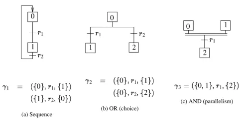
In the sequel a grafcet is given by the set of transitions. Graphical examples with their corresponding sets of transitions are pictured on Fig. 1.
2.3.1. Transition conditions
We first introduce transition conditions defined by terms over the flows and their edges. The set of transition conditions is the set of terms3over tt ff
inductively defined by:
tt ff , ,
(we note ¯ for ),
1 2 1 2 1 2 .
2this will be precisely defined later. 3we assume a particular grafcet under study.
0 1 1 2 1 0 1 1 1 2 0 (a) Sequence 1 1 0 2 2 2 0 1 1 0 2 2 (b) OR (choice) 0 1 2 1 3 0 1 1 2 (c) AND (parallelism)
Figure 1. Examples of grafcets
With each transition condition we associate a value " in the boolean set tt ff
depending upon " 2 and . The interpretation " for is defined
inductively: " tt tt, " ff ff, " tt if , ff otherwise, " " " tt , " ¯ " , " 1 2 " 1 " 2 , " 1 2 " 1 " 2 . 2.3.2. Evolution rules
State changes are determined in GRAFCET by five evolution rules [COM 88] [DA 89]:
rule 1 the initial situation !0 2 defines the active steps at the first instant,
rule 2 a transition is enabled if all its input steps are active; it is clearable if the two
following conditions hold: 1. it is enabled,
2. the transition condition evaluates to true. A clearable transition is immediatly cleared,
rule 3 clearing a transition yields the following changes:
the input steps are stopped, the output steps are activated,
rule 4 if many transitions are simultaneously clearable, they are simultaneously
cleared,
rule 5 if during an evolution a step must be both activated and stopped it remains
activate (this is stronger than the classical rule which states this only for active steps).
Definition 3 A basic evolution is a state change obtained by applying the five evolution
rules simultaneously to each transition. We denote a basic evolution from state on an occurrence of event
We do not use any subscript here to remind that this is a single evolution step.
2.4. Example 1
An example of a GRAFCET specification is given on Fig. 1.(a). with transition conditions 1 and 2 ¯. The initialstate of the system is 0 !0 "0
with !0 0 tt !0 1 ff, "0 "0 ff. In the remainding of the paper
we will use the shorter notation 0 0 ¯ ¯ (i.e. ! is replaced by ! 1 tt and for
we use if " tt, ¯ otherwise).
A possible interpretation of GRAFCET is the without stability search (WOSS) interpretation. It consists in processing new occurrences of events immediatly after each basic evolution. Then from state 0if event occurs the basic evolution of the
system is
0 0 ¯
1
4
Remark 2 In frequently used interpretations of GRAFCETthe value of the transition condition 1would be true. In our interpretation, the value of this transition condition
is ¯ which evaluates to false. However it is always possible to change
this interpretation and use instead of with " " where " denotes
the updated values of the flows after the edges of have occurred. The common interpretation assumes right continuity of the piecewise functions giving the values
of the flows. In this case a transition condition like is equivalent to in the sense that they are true at the very same time. Our choice is left continuity of the piecewise boolean functions: we consider that the values of the boolean variables will have changed only at the next state and that they are updated during the reaction. Thus is no longer equivalent to . The term in a time condition refers to the last persistent value of the flow . As our interpretation differs from the standard ones, we will use the term GRAFCETwhen we consider it. The interested reader is refered to [DLR 91] for a complete discussion of this subject.
From state 1, if no new event has occurred the transition condition 1 is now
true. 1is then a non stable state (since we can proceed further basic evolutions) and
the evolution rules for the WOSS interpretation implies that clearable transitions be immediatly cleared4: 1 1 0 1 ¯ 2 5
On the contrary if event has occurred during the basic evolution (4), the system reaches state 3instead of state 2:
1
1 0 1
3
Now considering the reactive assumptions stated at the beginning of this section we have: 1) a reaction takes no time: thus no changes can occur in a null duration; 2) if no changes can occur during a basic evolution the system state changes with the silent move (5) without any new occurrences of events. This is not compatible with the reactive notions and thus a basic evolution in the WOSR interpretation can not be taken as a reaction.
The intuitive semantics we are going to present in section 3 implements another interpretation of GRAFCET: the with stability search (WSS) interpretation. With this interpretation of GRAFCETnew events are not taken into account before a stable state has been reached. Then, from state 0, the basic evolutions leading to a stable state are
0 1
1 2 2
and the reaction of the system to event is
0
0 1 2
2.5. Example 2
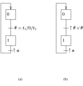
GRAFCETprovides for time condition that can be used to delay actions and handle
time units. They allow one to specify the application with a metric aspect of time that refers to the instants a step was started or stopped. A time condition is part of a transition condition: the grafcet pictured on Fig. 2.(a) has a time condition linking step 0 to step 1. A time condition is written 1 2with 1 2 IR and
(in standard GRAFCET 1 2 IN ). For 1 2, we note
( is the clock step of the time condition), 1and 2.
0 1 1 0 2 (a) 0 1 (b)
Figure 2. A grafcet with time condition
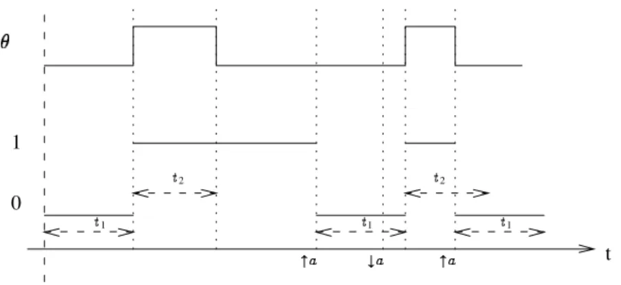
The intuitive semantics associated with a time condition is described on the time diagram Fig. 3:
1. at the initial instant is false,
2. step 0 is the only active step at the initial instant,
3. becomes true 1 time units after step 0 has been activated5; at this date the
transition condition involving is cleared and step 1 is started, step 0 is stopped,
5i.e., a stopwatch is started at the time step 0 is activated and after
1time units it ticks, step 0 being
4. becomes false 2time units after step 0 has been stopped6,
5. an occurrence of starts step 0 again,
6. if step 0 is started again before 2time units have elapsed, is reset to false.
1 0 2 2 1 1 1 t
Figure 3. Time diagram
It is obvious that time condition are flows (boolean values). In GRAFCET, time conditions are modelled with time condition boolean variables: the instants when the edges of these variables occur depend on the time elapsed since the starting or stopping of clock steps . In GRAFCET, a time condition 1 2is semantically defined
by a transition condition : the grafcet of Fig. 2.(a) is interpreted as Fig. 2.(b). For any grafcet , let be the set of all the time conditions. The values of the time conditions at any instant are given by
# 2 6
The set of transition conditions of GRAFCETis extended in GRAFCETto the time conditions: transition conditions in GRAFCET are terms built as described in section 2.3.1 with replaced by . However the use of the operator (not) on time condition is forbidden (this is not for semantic reasons: one may think of introducing a new feature in GRAFCET which is the negative time condition. This amounts to considering time intervals [ALL 81] and two operators and : such a notion has already been defined in [RLG 94]).
6another stopwatch is started at the instant step 0 is stopped and after
2time units it ticks unless step 0
The interpretation of the new terms is straighforwardly extended to time conditions and the new interpretation is noted " # . Finally a state is now a 3-tuple ! " #
in 2 2 2 . We use for the set of states 2 2 2 in the sequel.
2.6. Synchronism and asynchronism
Time conditions are viewed as boolean variables (like flows) the changes of which depend on an external clock. This is partial view of the time conditions as the metric part is left aside. This will enable us to build an abstract behavioural model for GRAF -CETprograms that will be “timed” later on. So far time conditions are particular flows. Occurrences of events from cannot be simultaneous as in the standard GRAF
-CETinterpretations. But two events of may occur at the same time; moreover they
sometimes do occur at the same time as in 1 1 2, 2 1 2 for which 1and 2are always simultaneous. The complete treatment of these situations is
defined in [CAS 95]. Then edges of time conditions variables are elements of . Finally, events of and cannot be simultaneous: we think that time condition events are to be processed with highest priority as they can not be delayed. Moreover, once the semantic model has been timed, the notion of an external clock is useless and state changes brought about by time conditions will be silent. From now on, a reaction has the following form
7
Remark 3 In GRAFCETtransition conditions may involve the activities of the steps
as in GRAFCET. This is developped in [CAS 95].
2.7. Stability
On the example of Fig. 2 we see that from state 1 ¯ ¯ there is a basic evolution to state
1 ¯ ¯
0 1 0 ¯ ¯
Is a stable state in the sense that there are no possible basic evolutions from this state? In standard GRAFCETinterpretations this state is stable only if 1 0, otherwise
it is non stable. With the WSR standard interpretation and 1 0 the next move is
1 0 1 ¯
and if 1 0 is stable.
In GRAFCET is a stable state: to leave this state we must wait for to occur. If 1 0 then this event will occur 0 time unit after has been entered.
intrinsic unstability which does not depend on any value (like 1) is called
structural unstability,
unstability that depends on time condition values (the previous case) is called
temporal unstability.
Temporal unstability will not be treated with the semantic rules and will be a property of the timed model defined in section 4.
3. Dynamic semantics for GRAFCET
This section formalizes the calculus of basic evolutions and reactions. The seman-tics is given with conditional rules in the style of Plotkin [PLO 81].
3.1. Notations
For a set , we note and for a set and for $ and for where
The previous definitions will be used to calculate the steps that are to be activated and stopped on a reaction or basic evolutions. $ allows us to calculate the set of steps that must be activated and deactivated when firing a transition. If and respectively denote the input and output steps of a transition and the set of active steps in the current state of the system, $ gives the set of output events corresponding to the firing of the transition: (resp. ) means that step is to be activated (resp. deactivated). According to rule 5, the activated steps are those which were not active in the last state. The operator extends $ to simultaneous firing of transitions. If taken independently, the firing of two transitions entail output events and , then when fired simultaneously, rule 5 applies: a step is activated if is activated by at least one of the firing, and deactivated if is not simulatneously activated.
To update the boolean variables we need the operator over 2 with value in 2 defined by :
" " " ¯ " " "
Similarly we introduce and over 2 and 2 with values in 2 and 2 to update the activities of the steps and the time condition variables. Finally for ! " # , and , we use the following abbreviation
! " #
3.2. Syntax of GRAFCET
A grafcet in GRAFCETis a directed graph the edges of which are elements of . As we want to give a structural operational semantics for GRAFCET
we define an abstract ambiguous grammar to describe the element of GRAFCET(the
axiom is %):
% :: (8)
% % (9)
with . If 1 2 , 1is the set of input steps and 2the
output steps. 3.3. Semantics
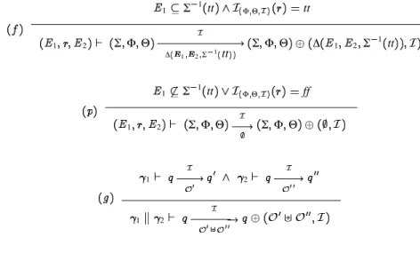
The calculus of basic evolution is formally defined by the structural operational semantics (SOS) given in Fig. 4. These rules express the five evolution rules listed in section 2.3.2.
For a grafcet , a state and an event , the basic evolution from on the occurrence of written
is the only one7that satisfies
1 ! 1 tt " # tt 1 2 ! " # $ 1 2! 1tt ! " # $ 1 2 ! 1 tt 1 ! 1 tt " # ff 1 2 ! " # ! " # 1 2 1 2
Figure 4. Operational semantics for GRAFCET
3.4. Properties of the semantics
Theorem 1 The operational semantics given for GRAFCETis deterministic and
com-plete. Moreover, the result does not depend on the derivation tree8
used for program %.
Proof of Theorem 1
Completeness is obvious from the rules of Fig. 4. Determinism relies on a property of operator . In a previous version of this article [CAS 96] the claim that commutativity of the operator was sufficient to ensure determinism was wrong: this mistake has been pointed out by Charles Andre´. We give here a correct proof for determinism.
We first establish that is associative. For this we need the following algebraic laws:
same for same for (the converse holds)
same for Now let be subsets of .
From the previous laws we infer that
which yields to
and as we obtain
A similar calculus can be carried out for ending with the same result which proves that is associative.
Now remark that in rule (g) of Fig. 4 the new state depends on the previous one and on and not on and written in the premisses. This ensures determinism. The commutativity (obvious) of the operator ensures that whatever the order the elements of the directed graph are listed in, the semantics of a grafcet is unique:
1 2 2 1
3.5. Structural stability
We define structural stability for a state ! " # , a grafcet and an output event , denoted inductively by :
if 1 2 then
if 1 2then
1 2
Definition 4 A pair with is stable for a grafcet iff ( ) tt.
A pair with is non stable.
3.6. Calculus of a reaction
Definition 5 The9reaction from state 0on an occurrence of event is
the sequence 0 1 2 of basic evolutions from 0such that 0 0 0 1
1
and for each 0,
1
1, and ( ) ff.
This sequence may be finite if there is a stable pair , and infinite otherwise. If the sequence is finite we write
0 1 1 1 2 1 1 1 with 1 1 . Otherwise 0 1 1 1 2 1 1
and IN ( ) ff. We denote the set of indices of the state of a reaction: if it is finite then 0 1, otherwise IN.
Definition 6 The orbit of a reaction from on is the set .
Proposition 1 , contains at most one stable pair
and if there is a stable pair in , this set is finite.
Proof of proposition 1
Direct from the definition 5 of a reaction.
Now let . To calculate the orbit we introduce a function for a given grafcet of GRAFCETdefined by :
:
such that
Remark 4 is a total function as the operational semantics is deterministic and complete. is an output event from .
We extend to :
:
Then, in the ordered set , the function is monotonic. From the well-known Tarski’s theorem [TAR 55] we deduce that the equation
with
has a least fixed point . As is finite with minimum element there exists IN such that . Moreover the following theorem holds :
Theorem 2 ,
Proof of theorem 2
Let 0 and 0 1 then IN . It suffices
to prove:
1. IN ,
2. IN si alors .
This is straightforward by induction on IN.
3.7. Reaction of the system
A reaction of the system is a sequence of basic evolutions. For and , the reaction of the system to is :
where:
if is infinite, and (the undefined state and undefined output event),
otherwise is finite, the reaction 0 1 2 converges ; let 1
! 1 " 1 # 1 , the steps to be activated and stopped and the updated
values of the boolean time condition variables are defined using the initial and final states and 1. The reaction is then defined to be where
! 1 " 1 # and: ! 11 tt ! 1 tt (started steps) ! 1 tt ! 11 tt (stopped steps) and # ff if , otherwise # # 1 .
This way, a step is considered to be activated (resp. stopped) if it was idle (resp. active) in and now is active (resp. idle) in . Similarly, we consider time condition to be set according to external time: the correction to the final state is defined according to what happened on the reaction and the values of the boolean time condition variables are set accordingly.
4. Finite state modeling of GRAFCET programs
The semantic model for GRAFCETprogram is given only for programs with at most one time condition (general case is in [CAS 95]). For a time condition we introduce two clock variables
measures the elapsed time since the last start action on , , measures the elapsed time since the last stop action on .
4.1. Awaited events
It is clear that a way of defining a semantic model for GRAFCETprograms would consist in exploring from any state all the possible transitions brought about by all the events of . In fact, not all events are possible from any state and it reduces the size of the model if we care for not introducing impossible transitions.
From a state ! " # , we define the awaited events to be " 1 tt " 1 ff
where if ! 1 tt # 1 ff , if ! 1 ff
Example For the grafcet of Fig. 2.(b), 1 . For state 5 1 ¯ ¯ ,
5 .
4.2. Liveness
The system can stay in a state as long as no edges occur. Edges for time conditions occur at definite date when and . Then staying in state
! " # entails the following inequations to hold: if # 1 ff ! 1 tt ,
if # 1 tt ! 1 ff , tt otherwise.
We note the inequation associated with state . Similarly, we need where is replaced by .
4.3. Behavioural model: Timed automaton
The behavioural model for an GRAFCETprogram is a timed automaton [NSY 92] [AD 90]. Let , et be the sets of steps, boolean variables and time condition variables for a grafcet . The initial state of the system is defined by 0 . The
behavioural model for grafcet is the timed automaton 0
where:
2 2 2 is the set of states,
0 !0 "0 #0 is defined by – !01 tt 0, ! 1 0 ff 0 – "0 ff , – #0 ff ,
is the set of timers of the automaton,
is such that ! " # ( is the set of boolean terms [NSY 92] over the variables of ),
where is defined inductively as follows:
2.
where and et
and .
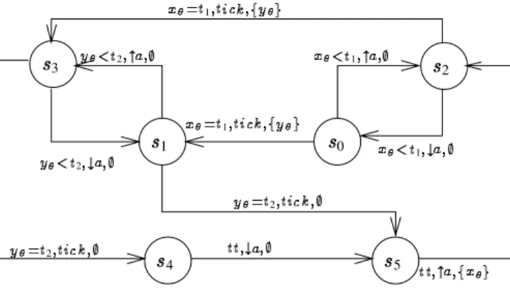
For the grafcet of Fig. 2.(b) we obtain the timed automaton given Fig. 510. The
states information is listed in Table 1.
state state information
0 0 ¯ ¯ 1 1 1 ¯ 2 2 0 ¯ 1 3 1 2 4 1 ¯ 5 1 ¯ ¯
Table 1. States information
3 2 0 1 4 5 1 1 2 1 1 2 2 2
Figure 5. Timed automaton
Remark 5 If 1 0 (Cf. 2.7), we move from state 5 to state 0 on an occurrence
of : in this state the condition 0 1 is true if time does not pass:
moving to state 1takes no time.
4.4. Stability
Structural stability It is quite obvious that a couple is non stable if is infinite. In this case the corresponding reaction is defined as in section 3.7.
Let be a particular grafcet. An endless (undefined) reaction is possible only if state is reachable in the associated automaton .
We will not discuss here the decidability of this problem [ACH 95] [KPSY 93] [RR 96b] [RR 96a]: in fact it has so far been proved decidable only for bounded reachability (i.e. reachability within a given time interval).
Temporal stability Temporal stability occurs only if there is a cycle in the automaton
on which time does not progress. Checking the automaton for temporal stability then amounts to a reachability problem within a time interval of null duration. Again we refer the reader to [ACH 95] [KPSY 93] [RR 96b] [RR 96a] for a discussion on these problems.
5. Conclusion
The work presented in this paper differs from the ones where GRAFCETis translated
in a reactive language [RR 94] [AP 92] [ML 92] since we model the metric aspect of time. The semantics given above is based on the idea of [AG 94] where the evolution rules are characterized by fixpoints11; our semantics include the time conditions.
We have shown in this article that an operational semantics could be defined for GRAFCETgiving this language a formal background. This semantics associates with a grafcet a timed automaton. A compiler from GRAFCETto timed automata has been written inCAML[LW 93] [WL 93]. On non trivial examples the size of the associated automaton is rather small with respect to the maximum number of possible states (2 ) as shown on Table 2. We may then think of verifying “real” grafcets with tools likeVALET[RUS 96] or KRONOS[YOV 93] (although those tools can right now only handle small systems).
Moreover, the model (namely a timed automaton) can be enriched to include the actions of GRAFCETto obtain a more accurate model of the system: the enriched model is then a hybrid system [ACH 95] [NOSY 93]. We then use the toolVALET[RUS 96] developped at L.A.N. (Nantes) to check properties on particular classes of hybrid
Steps Flows Time conditions Edges 2 Number of states
3 1 2 3 64 15
5 2 3 6 1024 142
8 3 0 7 2048 40
12 7 1 11 1 048 576 1952
Table 2. Sizes of the automata
systems [RR 96b] [RR 96a]: this tool provides for the use of stopwatches (i.e. clocks that can be stopped and restarted later) when KRONOSonly handles timed automata.
The author wishes to thank Charles Andre´ for his careful reading of the many versions of the paper and the other anonymous referees for their comments which helped us to improve many parts of this work.
6. References
[AA 92] ADEPA-AFCET. Le Grafcet. Ce´padues, 1992.
[ACH 95] R. Alur, C. Courcoubetis, N. Halbwachs, T. Henzinger, P. Ho, X. Nicollin, A. Oliv-ero, J. Sifakis, and S. Yovine. The algorithmic analysis of hybrid systems.
Theo-retical Computer Science B, 137, January 1995.
[AD 90] Rajeev Alur and David Dill. Automata for modelling real-time systems. In Lecture
Notes in Computer Science, volume 443, pages 322–336. Springer–Verlag, July
1990.
[AFC 77] AFCET. Normalisation de la repre´sentation du cahier des charges d’un automatisme logique. Automatique et Informatique Industrielle, 1977.
[AFN 82] AFNOR. Norme C03–190, 1982. Paris (FRANCE).
[AG 94] Charles Andre´ and Daniel Gaffe´. E´ve´nements et Conditions en GRAFCET.
Au-tomatique Productique et Informatique Industrielle, 28(4):331–352, 1994.
[ALL 81] J.F. Allen. An interval-based representation of temporal knowledge. In Proceedings
of the IJCAI’81, pages 221–226, Vancouver, August 1981.
[AP 92] Charles Andre´ and Marie-Agne`s Peraldi. GRAFCETet langages synchrones. In
GRAFCET’92 Conf., Paris, march 1992.
[BB 91] Albert Benveniste and Ge´rard Berry. The synchronous approach to reactive and real-time systems. Proceedings of the IEEE, 79(9):1270–1282, september 1991. [BD 91] Fre´de´ric Boussinot and Robert De Simone. TheESTERELlanguage. Proceedings
of the IEEE, 79(9):1293–1304, september 1991.
[BG 91] Ge´rard Berry and Georges Gonthier. TheESTERELsynchronous language: design, semantics, and implementation. Science of Computer Programming, 1991.
[BRA 83] G. W. Brams. Re´seaux de Pe´tri: The´orie et Pratique. MASSON, 1983. Tomes 1–2. [CAS 95] Franck Cassez. GRAFCET : Un GRAFCET re´actif. Research Report RR –95– 01, De´partement d’Informatique, Universite´ de Bretagne Occidentale, 6, Avenue Le Gorgeu B.P. 809 29285 Brest Cedex (FRANCE), 1995.
[CAS 96] Franck Cassez. Une se´mantique pour GRAFCET re´actif. In Mode´lisation des
syste`mes re´actifs, pages 373–380, Brest (FRANCE), March 1996.
[COM 88] International Electrotechnical Commission. Preparation of function charts for con-trol systems, IEC 848, 1988.
[COM 93] International Electrotechnical Commission. IEC 1131 standard for programmable controllers, part 3: Programming languages, 1993.
[CPHP 87] Paul Caspi, Daniel Pilaud, Nicolas Halbwachs, and John A. Plaice. LUSTRE: a declarative language for programming synchronous systems. In Proceedings of
the 14 ACM Symposium on Principles of Programming Languages, Munich
(GERMANY), january 1987.
[CR 95] Franck Cassez and Olivier Roux. Compilation of the ELECTRE reactive language into finite transition systems. Theoretical Computer Science B, 146(1–2):109–143, July 1995.
[DA 89] Rene´ David and Hassane Alla. DuGRAFCET aux re´seaux de Petri. Editions
HERMES, Paris, 1989.
[DLR 91] B. Denis, J-J. Lesage and J-M. Roussel. A boolean algebra for a formal expression of events in logical systems. Proceedingsof the IMACS Mathmod, Vienna (Austria), pages 859–862, February 1994.
[ER 85] Jean-Pierre Elloy and Olivier Roux.ELECTRE: A language for control structuring in real time. The Computer Journal, 28(5), july 1985.
[HAR 87] David Harel. STATECHARTS: a Visual Formalism for Complex Systems, volume 8,
pages 231–274. North Holland, june 1987.
[HCRP 91] Nicolas Halbwachs, Paul Caspi, Pascal Raymond, and Daniel Pilaud. The syn-chronous dataflow languageLUSTRE. Proceedings of the IEEE, 79(9):1304–1320, september 1991.
[KPSY 93] Y. Kesten, A. Pnueli, J. Sifakis, and S. Yovine. Integration graphs: a class of decidable hybrid systems. In R.L. Grossman, Nerode, A.P. Ravn, and H. Richel, editors, Workshop on Theory of Hybrid Systems, pages 179–208, Lyngby, Denmark, June 1993. Lecture Notes in Computer Science 736, Springer-Verlag.
[LBBG 86] Paul Le Guernic, Albert Benveniste, Patricia Bournai, and Thierry Gautier.SIGNAL: a data-flow oriented language for signal processing. IEEE transactions on ASSP, ASSP-34(2):362–374, 1986.
[LLGL 91] Paul Le Guernic, Michel Le Borgne, Thierry Gautier, and Claude Le Maire. Programming real-time applications with SIGNAL. Proceedings of the IEEE,
79(9):1321–1336, september 1991.
[LW 93] Xavier Leroy and Pierre Weis. Manuel de re´fe´rence du langageCAML. InterE´ ditions, 1993.