General stochastic reverberation model

— We describe the inner structure of stochastic automata over measurable spaces by their lattice of congruences, where a congruence is given by a diminished set of possible events

completely weak provided that every loop isotopic to L satisfies the weak inverse property.. Such loops have been studied by

We aimed to evaluate edentulous pa- tients with regards to the relationship between dimensions, bone characteristics, cancellous densities, and cortical thickness of the

The stars are dead but their light lives on, installation view at Eastern Bloc, 2013 production residency film stills, 2014. an Ontario government agency un organisme

In [17, Table 1] the list of possible minimal zero support sets of an exceptional extremal matrix A ∈ COP 6 with positive diagonal has been narrowed down to 44 index sets, up to

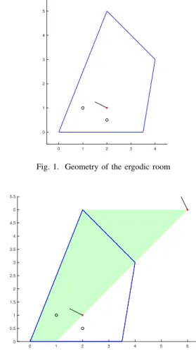
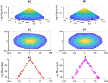
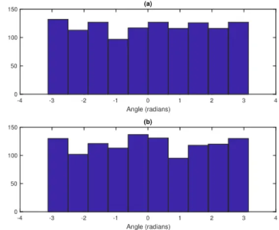
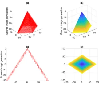
Rather than setting an arbitrary threshold on modal overlapping as a necessary condition for an overmoded behaviour, the statistical uncertainty due to the limited number of

This version of the Ward identity is valid only if proper Green's functions involving gluons of all four polarizations are free of singularities when any of the p+'s become zero;

Importantly, the impact of agreement or positive social feedback on subjective confidence ratings was greater when it was provided by a competent rather than an incompetent

REFERENCES

[1] R. Badeau, “Common mathematical framework for stochastic rever-beration models,” The Journal of the Acoustical Society of America, 2019, Special issue on room acoustics modeling and auralization. To be published.
[2] R. K. Cook, R. V. Waterhouse, R. D. Berendt, S. Edelman, and M. C. Thompson Jr., “Measurement of correlation coefficients in reverberant sound fields,” The Journal of the Acoustical Society of America, vol. 27, no. 6, pp. 1072–1077, 1955.
[3] M. R. Schroeder, “Frequency-correlation functions of frequency re-sponses in rooms,” The Journal of the Acoustical Society of America, vol. 34, no. 12, pp. 1819–1823, 1962.
[4] M. R. Schroeder and K. H. Kuttruff, “On frequency response curves in rooms. Comparison of experimental, theoretical, and Monte Carlo results for the average frequency spacing between maxima,” The Journal of the Acoustical Society of America, vol. 34, no. 1, pp. 76–80, 1962. [5] J. A. Moorer, “About this reverberation business,” Computer Music
Journal, vol. 3, no. 2, pp. 13–28, 1979.
[6] M. R. Schroeder, “Statistical parameters of the frequency response curves of large rooms,” The Journal of the Audio Engineering Society, vol. 35, no. 5, pp. 299–306, 1987.
[7] J. D. Polack, “La transmission de l’énergie sonore dans les salles (The transmission of sound energy in rooms),” Ph.D. dissertation, Université du Maine, Le Mans, France, 1988.
[8] J.-D. Polack, “Modifying chambers to play billiards: the foundations of reverberation theory,” Acta Acustica united with Acustica, vol. 76, no. 6, pp. 256–272(17), Jul. 1992.
[9] ——, “Playing billiards in the concert hall: The mathematical founda-tions of geometrical room acoustics,” Applied Acoustics, vol. 38, no. 2, pp. 235–244, 1993.
[10] J. B. Allen and D. A. Berkley, “Image method for efficiently simulating small-room acoustics,” Journal of the Acoustical Society of America, vol. 65, no. 4, pp. 943–950, 1 1979.
[11] H. Kuttruff, Room Acoustics, Fifth Edition. Boca Raton, FL, USA:
Figure
Fig. 2. Closest top-right source image and its visibility region
Fig. 3. Two constellations of source images up to 30th generation
Fig. 6. Reflection cones of the log-magnitudes of the source images (attenuations do not depend on the angle of incidence on the walls)
Fig. 2 shows that the orientations of the source images are obtained by iteratively mirroring that of the original source.
+4
Références
Documents relatifs