Robust optimization of a 2D air conditioning duct using kriging

HAL Id: hal-00566285

https://hal.archives-ouvertes.fr/hal-00566285

Submitted on 15 Feb 2011

HAL is a multi-disciplinary open access

archive for the deposit and dissemination of

sci-entific research documents, whether they are

pub-lished or not. The documents may come from

teaching and research institutions in France or

abroad, or from public or private research centers.

L’archive ouverte pluridisciplinaire HAL, est

destinée au dépôt et à la diffusion de documents

scientifiques de niveau recherche, publiés ou non,

émanant des établissements d’enseignement et de

recherche français ou étrangers, des laboratoires

publics ou privés.

Robust optimization of a 2D air conditioning duct using

kriging

Janis Janusevskis, Rodolphe Le Riche

To cite this version:

Janis Janusevskis, Rodolphe Le Riche. Robust optimization of a 2D air conditioning duct using

kriging. 2011. �hal-00566285�

Robust optimization of a 2D air conditioning duct using kriging

Deliverable WP.2.2.2.B of the ANR / OMD2 project

Janis Janusevskis

_{and Rodolphe Le Riche}

_{LSTI / CROCUS team}

Ecole Nationale Sup´erieure des Mines de Saint-Etienne

Saint-Etienne, France

2

_{CNRS UMR 5146}

{janusevskis,leriche}@emse.fr

Abstract

The design of systems involving fluid flows is typically based on computationally intensive Computational Fluid Dynamics (CFD) simulations. Kriging based optimization methods, especially the Efficient Global Optimization (EGO) algorithm, are now often used to solve deterministic optimization problems involving such expensive models. When the design accounts for uncertainties, the optimization is usually based on double loop approaches where the uncertainty propagation (e.g., Monte Carlo simulations, reliability index calculation) is recursively performed inside the optimization iterations. We have proposed in a previous work a single loop kriging based method for minimizing the mean of an objective function: simulations points are calculated in order to simultaneously propagate uncertainties, i.e., estimate the mean objective function, and optimize this mean.

In this report this method has been applied to the shape optimization of a 2D air conditioning duct. For comparison purposes, deterministic designs were first obtained by the EGO algorithm. Very high performance designs were obtained designs, but they are also very sensitive to numerical model parameters such as mesh size, which suggests a bad consistency between the physics and the numerical model.

The 2D duct test case has then been reformulated by introducing shape uncertainties. The mean of the duct performance criteria with respect to shape uncertainties has been maximized with the simultaneous optimization and sampling method. The solutions found were not only robust to shape uncertainties but also to the CFD model numerical parameters. These designs show that the method is of practical interest in engineering tasks.

1

Introduction

The analysis of systems involving fluid flows often is assisted with Computational Fluid Dynamics (CFD) simulation models. Solving procedures of such models usually involve computationally intensive algorithms, therefore to reduce time needed for optimization, metamodels (also known as approximations, response surfaces or surrogate models) are used. Kriging or Gaussian Process (GP) regression [14, 13] has become a popular metamodeling tool for computation-ally expensive simulators as it provides surfaces of tunable complexity (possibly interpolative) within a probabilistic framework. The Efficient Global Optimization (EGO) algorithm [8, 7] is based on kriging metamodels which allow formulate Expected Improvement (EI) criterion for optimization of deterministic simulators.

However, real life problems are almost always non-deterministic. Uncertainties appear for example due to model errors, manufacturing tolerances, changing environments and noisy measurements. A kriging based method allowing to minimize mean response has been proposed in [6]. In this report this method is applied to the shape optimization of a 2D air conditioning duct. The uncertainties affect the pipe shape. The mean response, expressed in terms of pressure drop and velocity variation at the duct outlet, is minimized in order to obtain a design robust to shape variations.

2

Problem formulation

The kriging based method for optimizing the mean of a perturbed objective function proposed in [6] is applied to a CFD problem: to optimize in two dimensions the shape of an air conditioner pipe subject to shape uncertainties. This is the test case 1 of the ANR / OMD2 project [1] with added uncertainties.

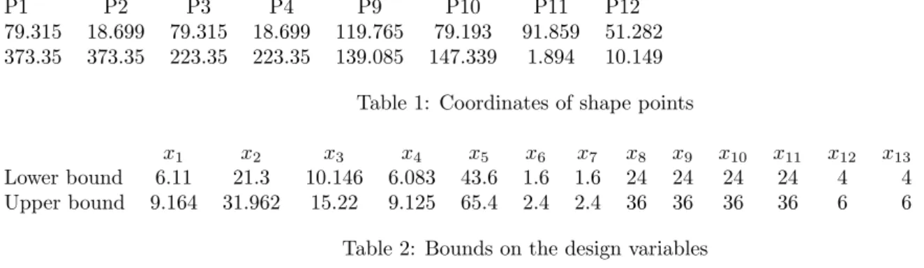
The shape of the pipe is described by line segments and Bezier curves. The pipe consists of 3 parts, visible in both Figures 1 and 3: the input pipe (P1-P2-P4-P3), the inner block, joining P3-P4 to P9-P10 and described by the shape variables x, and the output pipe (P9-P10-P12-P11). Two sets of shape parameters x will be discussed in Sections 3 and 4, respectively.

The CFD model is created and solved using the OpenFoam package [9]. The duct is discretized in 19000 finite elements with the OpenFoam mesher, with 50 cells along the X direction and a single cell along the Z direction. The

P1 P2 P3 P4 P9 P10 P11 P12 79.315 18.699 79.315 18.699 119.765 79.193 91.859 51.282 373.35 373.35 223.35 223.35 139.085 147.339 1.894 10.149

Table 1: Coordinates of shape points

x1 x2 x3 x4 x5 x6 x7 x8 x9 x10 x11 x12 x13

Lower bound 6.11 21.3 10.146 6.083 43.6 1.6 1.6 24 24 24 24 4 4 Upper bound 9.164 31.962 15.22 9.125 65.4 2.4 2.4 36 36 36 36 6 6

Table 2: Bounds on the design variables

boundary conditions impose a uniform velocity along the Y direction at the input (P2P1) and zero pressure at the output (P11P12) of the pipe. The steady-state solver simpleFoam for the Navier-Stokes equations of an incompressible, non-turbulent flow is used with kinematic fluid viscosity of 1.6e-04 m2_s−1_.

The deterministic optimization formulation, which overlooks shape uncertainties, has two objectives. The first objective is to maximize flow uniformity at the exit block (P10P9) or, more precisely, to minimize the standard deviation of the scalar projection of the flow velocity on the vector perpendicular to the P10P9,

minx∈DFlowSD(x)

such that xl_{≤ x ≤ x}u (1)

where xl_{and x}u_{are lower and upper bounds on x.}

The second objective is to minimize the pressure difference between input (P1-P2) and output (P11-P12) minx∈DPressureLoss(x)

such that xl≤ x ≤ xu

. (2)

The robust optimization problem additionally considers that some of the CFD model parameters are uncertain, and should therefore be described as random variables, U . A double set of parameters, x for the deterministic optimization variables and U for the random, uncontrolled parameters, is general as has been previously discussed in [12, 16, 15]. In the case of the air duct, U is a perturbation of the position of the outlet. A more precise description of U will be given in Section 4.2. The robust optimization problem is formulated as

minx∈DEU[flowSD(x, U )]

such that xl≤ x ≤ xu (3)

or

minx∈DEU[pressureLoss(x, U )]

such that xl_{≤ x ≤ x}u_. (4)

In both deterministic and robust formulations, the two performance criteria (pressure loss and flow standard deviation) are handled separately i.e. two shape optimization problems are solved.

The deterministic optimization problem is tackled with an EGO algorithm [8] while the mean response optimization is solved by the specialized “simultaneous optimization and sampling” EGO algorithm described in [6]. Both algorithms create x iterates by maximizing expected improvements (EI), although these EIs are different in both methods. Bounds on x variables are handled during the EI maximization : our implementation, which makes the Scilab KRISP toolbox (KRIging based regression and optimization Scilab Package, [5]), maximizes the EIs with a CMA-ES algorithm [4]. CMA-ES produces new x’s by sampling a Gaussian distribution. To handle bounds on x, the sampling is repeated until points are in-bounds.

3

Deterministic optimization with the original set of shape parameters

A sketch of the original shape parameters definition, i.e., the parameters such as described in the initial test case of the OMD2 project [1], is given in fig. 1. Coordinates of the shape points can be found in table 1. The shape geometry is defined by 13 parameters. The first 5 variables determine the rectangular inner block. The next 8 parameters determine the curvatures of the Bezier curves that connect the inner block to the P3-P4 input and the P10-P9 output parts. The bounds on the design variables are shown in table 2.

The original 13 parameter optimization problem is solved using the EGO algorithm. The initial random Latin Hypercube design (RLHD) [2, 10] consists of 200 points. 300 additional points are generated by EGO. The obtained optimum designs and associated criterion values are shown in table 3. The design shapes are drawn in fig. 2.

Two observations stem from these original optimizations. Firstly, as can be seen by comparing table 3 and table 2, the optimal designs are obtained for shapes where some of the variables are on the boundary of the design space. For

Figure 1: Description of the initial shape optimization variables for a 2D air conditioning duct. The first 5 variables determine the position and shape of the rectangular inner block. The next 7 parameters determine the curvature of the Bezier curves (1,2,3,4).

FlowSD Pr.Loss x1 x2 x3 x4 x5 x6 x7 x8 x9 x10 x11 x12 x13

0.415 2.024 6.11 31.962 10.146 9.125 65.4 1.6 1.6 36 24 36 36 4 4 0.481 1.855 6.11 31.962 10.156 8.257 54.45 1.77 2 34.443 24 25.926 27.398 4 4 Table 3: Criteria values and design variables of the optimal designs obtained from the original parameter definition. These designs solve eq. (1) (first row) and eq. (2) (second row).

(a) Design

min-imizing the

standard deviation of flow velocity, eq. (1)

(b) Design mini-mizing the pressure loss, eq. (2)

Criterion θ1 θ2 θ3 θ4 θ5 θ6 θ7 θ8 θ9 θ10 θ11 θ12 θ13

FlowSD 1. 0.260 0.476 1. 0.235 1. 1. 1. 1. 1. 1. 1. 1. PressureLoss 1. 0.270 0.479 1. 0.221 1. 1. 1. 1. 1. 1. 1. 1.

Table 4: Kriging scale hyper-parameters θi for Gaussian covariance kernel for 498 points LHD. Estimation based on

likelihood maximization. Parameters are rescaled to (0, 1]. x1 x2 x3 x4 x5

Lower bound 10 160 80 160 1 Upper bound 79 210 149 210 50

Table 5: Bounds on new design variables.

minimum standard deviation of velocity all of the variables are on the boundary of the design space, for minimum pressure drop 6 out of 13 parameters are on the boundary of the design space. Secondly, the current parametrization allows only subset of designs where the extensions of P4P3 and P5P6 cross each other in the positive x direction (it is possible to achieve only shapes where the block P5P6P8P7 is tilted counter clockwise). For these reasons, a new set of shape parameters is defined in the next section.

4

Optimization with new shape parameters

Anticipating the introduction of uncertain parameters U , we have sought when defining a new set of shape variables xto keep the numerical complexity of the test case limited by reducing the number of variables. A sensitivity analysis has been performed which, in concordance with the rest of this work, is based on kriging. Table 4 shows the scale hyper-parameters θi estimated by likelihood maximization on the 2D air conditioning duct problem with the initial

set of variables. In the current context of Gaussian kernels, the correlation between the performance F at two points x1 and x2_is Corr(F (x1), F (x2)) = exp − n X i=1 |x1 i − x2i|2 2θ2 i

One can see in table 4 that the 8 last θ’s estimates are large (actually on their upper bound), suggesting that the correlations are near 1 along these dimensions, i.e. the functions are almost flat in these directions. These last 8 variables correspond to the curvatures of the Bezier curves. In the new set of parameters, Bezier curvatures are therefore removed from the optimization and kept constant to a value such that connections between the inner quadrilateral and the entry and exhaust ducts are almost linear.

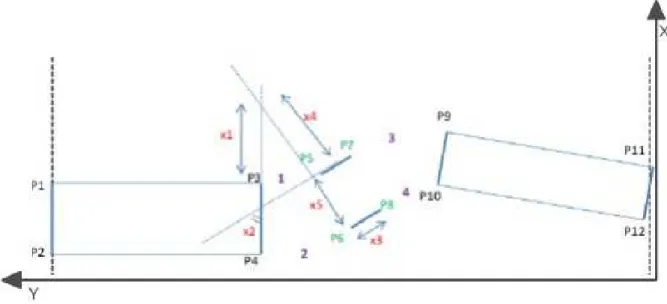
The five remaining variables are redefined as illustrated in fig. 3. The pipe consists of 3 rectangular blocks: B1 is a fixed input block, B3 is a fixed output block and B2 is a rectangular block of variable size and position that determines the shape of the pipe. The five shape parameters determine the size and position of the inner block (B2) and are optimized. Such re-parametrization of the problem leads to a more interesting test case as the domain of possible shapes is enlarged. In particular, it should be noticed that the designs of minimum flow standard deviation may only be achieved in the re-parametrized formulation, because their inner block B2 makes a negative angle with the X axis, see fig. 4 and fig. 5.

4.1

Deterministic design

Solutions to eq. (1) and eq. (2) are sought in a design space D ⊂ R5_{with the bounds given in table 5. These problems}

are approached with the EGO algorithm. During the optimization two practical problems have to be addressed. Firstly, some of the design points requested by the optimizer cannot be simulated due to geometrical infeasibility or CFD solver errors. We call such points non calculable (infeasible may be confusing as it is often used for points that do not satisfy optimization constraints). For example, geometrical infeasibility occurs when a part of B2 intersects B3 (x5is large and simultaneously x2 and x4are small). During the optimization procedure, infeasible geometries should

be diagnosed by the automatic mesher and/or the CFD solver software and the optimizer should be updated so as to move away from such non calculable designs. A typical solution is to penalize the performance of such points to force the optimizer away from the non calculable region. For example in the EGO optimizer of [3], non calculable points are assigned a penalized performance equal to the sum of predicted kriging mean and variance.

Here non calculable designs are assigned the predicted kriging 90th percentile, E (Yt_{(ω))+ 1.282pVAR (Y}t_{(ω)), where}

Yt_{(ω) is the conditional gaussian process (the kriging model). At every iteration we learn kriging hyper-parameters}

without non calculable points. For calculation of EI we use the updated kriging model (with the newly estimated hyper-parameters) and all sampled points, including the non calculable ones with the 90th percentile as performance

Figure 3: Sketch of the 2D air conditioning duct new parameters. 5 variables determine the position and size of the inner block B2. One variable, U1, randomly perturbs the horizontal positions of the exit block B3.

Original size mesh Double size mesh FlowSD 0.1422137 0.5320028 Pressure Loss 0.6040481 2.355656

Table 6: Criteria increase for optimal designs of deterministic formulations when doubling the mesh size.

value.

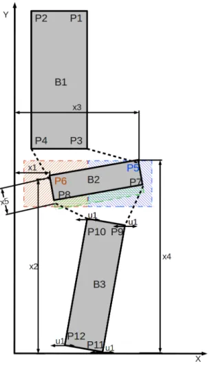
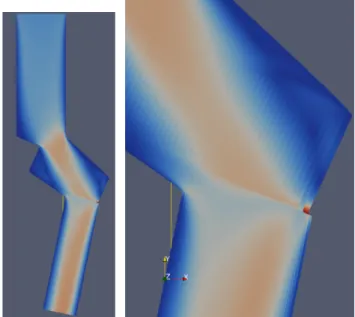
The second endemic problem is simulation inaccuracies that create false high performance designs: in some cases, our CFD model estimates that a design has a high performance, but the simulation does not properly describe the underlying physics. Examples of such designs are shown in fig. 4. The optimizer is fooled and attracted by these false designs. They are more complicated to diagnose on-line as non calculable designs. A possible test is to modify the numerical model (increase mesh size) and recalculate these designs. Table 6 shows that doubling the mesh size on the deterministic numerical optima of fig. 4 increases their objective functions considerably. The first row in table 6 gives the ever best standard deviation of flow velocity found. The value of 0.1422137 increases to 0.5320028 as the mesh size is doubled. The second row provides the ever best calculated pressure loss criterion which increases from 0.6040481 to 2.355656 as the mesh size is doubled. This fact shows that the first simulations of these designs do not correctly capture the involved physical phenomena.

An often useful yet computationally costly test is thus to change the mesh and check that the simulation output is sufficiently stable. It is costly because the simulation needs to be repeated and it is not trivial to decide during an optimization what is “sufficiently stable”. Because false designs are also sensitive to shape variations, robust optimization techniques are another way of avoiding them as will be seen in the next section.

4.2

Duct design with uncertainties

We now address the problems eq. (3) and eq. (4) where the uncertain parameter U is introduced and where the mean response is minimized to obtain robust designs.

4.2.1 Definition of the uncertainties

Several definitions of the uncertain parameter U have been tried. At first, we have perturbed the air velocity at the input of the pipe. The perturbation was either a Gaussian noise added to the y velocity component (the x component is zero), or a Gaussian noise added to the x velocity component. Both definitions did not lead to an interesting test case as the designs are not sensitive to perturbations of the input velocity: the deterministic designs, even the false ones of fig. 4, remain optimal.

In the final version of the test case, uncertainties affect the duct shape. A gaussian noise is added to the x position of the exit tube B3, cf. fig. 3. The mean and standard deviation of this noise are µ = 0 and σ = 3 (5% of the width of the exit tube), respectively.

4.2.2 Definition of what is the best design in the presence of uncertainties

The definition of the best design at the end of the search deserves further explanations because its performance is not directly observed : during the optimization, the mean performance is estimated through a conditioned and averaged Gaussian process. We define as “best design” that which minimizes the 90% quantile of the mean and which has received at least one observation in deterministic x variable space :

x= arg min x∈X Eh_Z(x)t _(ω)i_{+ 1.282} r VARh_Zt (x)(ω) i ! . (5) where Zt

(x)is the mean process

Z_(x)t = EUY(x,U )t

and Yt

(x,u) is the kriging (conditional process) build from t observations of the response function, here either the

pressure loss or the velocity variation. X is the subset of already calculated deterministic variables, {x1_{, . . . , x}t_}.

Again, more details on the mean process Z can be found in [6]. By such a procedure the obtained solutions have been observed at least once for the given x and the quantile favors designs that are well known under the kriging usual assumptions.

(a) Design maximiz-ing flow uniformity

(b) Zoomed in design maximizing flow uniformity

(c) Design minimiz-ing pressure loss

(d) Zoomed in desing minimizing pressure loss

Figure 4: Numerically optimal or false designs of deterministic formulation. High performance values are due to locally highly distorted meshes. The performance of these designs is not stable to meshes changes and small shape perturbations.

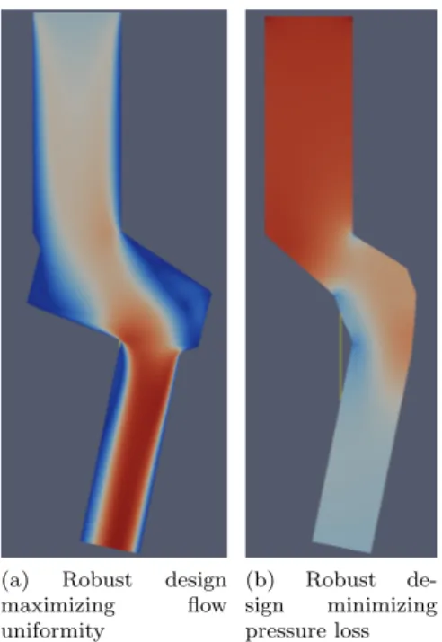
(a) Robust design maximizing flow uniformity (b) Robust de-sign minimizing pressure loss

Figure 5: Optimal duct for mean performance under shape uncertainties. Compare them to the deterministic designs in fig. 4.

Predicted mean by mean process Original mesh size (19000 cells) Double mesh size (38000 cells)

FlowSD 0.1747401 0.1694480 0.2326873

Pressure Loss 1.6154491 1.9856566 2.0780128

Table 7: Robust designs performance criteria and variation under mesh changes. These designs are solutions to eq. (3) and eq. (4).

4.2.3 Results

The initial random latin hypercube design of the simultaneous optimization and sampling algorithm [6] consists of 200 points in six dimensions ((x, u) parameter space made of five x’s and one u). The optimization is run for 400 additional points (i.e., 400 iterations).

Using such formulation and optimization approach, the designs represented in fig. 5 are obtained. The performance criteria values of these designs are shown in table 7. By definition, these designs solve the mean performance problems, eq. (3) or eq. (4), and thus have better mean objective functions in comparison to the deterministic designs of fig. 4.

In addition, as can be seen in table 7, the robust designs are less sensitive to the mesh sizes. Compared to the deterministic optimization solutions, fig. 4, the obtained shapes, pressure and velocity plots appear smoother without high concentration at isolated locations, suggesting a better correspondence with the actual physical processes. The simultaneous optimization and sampling method for optimization of the mean therefore appears as a way to avoid what we have called false optima. The approach is numerically more efficient than doubling the mesh size at simulated points because, thanks to the kriging, design points do not have to be evaluated twice.

5

Conclusions

In this report, the simultaneous optimization and sampling method presented in [6] has been applied to the shape optimization of two-dimensional air conditioning duct. For comparison purposes, the design was first carried out by the EGO algorithm through a deterministic optimization problem formulation. Very high performance designs were calculated, thus confirming that EGO is an appropriate approach for the optimization of computationally expensive models such as CFD. However the obtained designs are very sensitive to the parameters of the numerical model (here the mesh size), which suggests a bad consistency between the physics and the numerical model. The 2D air duct test case has then been reformulated by introducing shape uncertainties. The mean of the duct performance criteria with respect to shape uncertainties have been maximized with the simultaneous optimization and sampling method. The solutions found were not only robust to shape uncertainties but also the CFD model numerical parameters. These

design show that the method is of practical interest in engineering tasks.

References

[1] ANR OMD2 project. http://omd2.scilab.org/, 2010.

[2] Peteris Audze and Eglajs Vilnis. New approach for design of experiments. Problems of Dynamics and Strengths, 35:104–107, 1977. (in Russian).

[3] A. I. J. Forrester, A. S´obester, and A. J. Keane. Optimization with missing data. Proc. R. Soc. A, (462):935–945, 2006.

[4] N. Hansen. The CMA evolution strategy: a comparing review. In J.A. Lozano, P. Larranaga, I. Inza, and E. Ben-goetxea, editors, Towards a new evolutionary computation. Advances on estimation of distribution algorithms, pages 75–102. Springer, 2006.

[5] Janusevskis J. KRIging Scilab Package. http://atoms.scilab.org/toolboxes/krisp/, 2011.

[6] Janis Janusevskis and Rodolphe Le Riche. Simultaneous kriging-based sampling for optimization and uncertainty propagation. Technical report, Equipe : Calcul de Risque, Optimisation et Calage par Utilisation de Simulateurs - CROCUS-ENSMSE - UR LSTI - Ecole Nationale Sup´erieure des Mines de Saint-Etienne, July 2010. Deliverable no. 2.2.2-A of the ANR / OMD2 project available as http://hal.archives-ouvertes.fr/hal-00506957. [7] Donald R. Jones. A taxonomy of global optimization methods based on response surfaces. Journal of Global

Optimization, 21:345–383, 2001.

[8] Donald R. Jones, Matthias Schonlau, and William J. Welch. Efficient global optimization of expensive black-box functions. Journal of Global Optimization, 13(4):455–492, 1998.

[9] OpenCFD Ltd. OpenFoam package. http://www.openfoam.com/, 2010.

[10] M. D. McKay, R. J. Beckman, and W. J. Conover. A comparison of three methods for selecting values of input variables in the analysis of output from a computer code. Technometrics, 21(2):239–245, 1979.

[11] Nikolaus Hansen. CMA-ES Source Code . http://www.lri.fr/~hansen/cmaes_inmatlab.html.

[12] G. Pujol, R. Le Riche, O. Roustant, and Bay X. L’incertitude en conception: formalisation, estimation. In

Optimisation Multidisciplinaire en M´ecaniques : r´eduction de mod`eles, robustesse, fiabilit´e, r´ealisations logicielles, M´ecanique et Ing´enierie des Mat´eriaux series. Hermes publisher, 04 2009.

[13] Carl E. Rasmussen and Christopher K. I. Williams. Gaussian Processes for Machine Learning (Adaptive

Com-putation and Machine Learning). The MIT Press, December 2005.

[14] Jerome Sacks, William J. Welch, Toby J. Mitchell, and Henry P. Wynn. Design and analysis of computer experiments. Statistical Science, 4(4):409–423, November 1989.

[15] G. Taguchi. System of experimental designs, volumes 1 and 2. UNIPUB/Kraus International Publications (White Plains, N.Y. and Dearborn, Mich.), 1987.

[16] Brian J. Williams, Thomas J. Santner, and William I. Notz. Sequential design of computer experiments to minimize integrated response functions. Statistica Sinica, (10):1133–1152, 2000.

6

Appendix: conditioner test case implementation

The test case was implemented using OpenFoam and Scilab code which is submitted along with this report as a deliverable.

6.1

Assumptions about OpenFoam installation

The attached code is working with Scilab version 5.2 and OpenFOAM version 1.6. It uses OpenFoam executables blockMesh for mesh generation and simpleFoam for solving. The OpenFoam case is defined under folder ./OpenFoam/. The Scilab scripts for generating test case are located in forlder ./scilab/.

The Scilab code implementing the minimization of mean response is located in folder ./rego toolbox/. It uses Scilab kriging package KRISP [5] and CMAES toolbox [11].

Optimization criteria x1 x2 x3 x4 x5 OpenFoam folder for design

FlowSD 23.919734 210. 141.33995 180.32402 37.224836 ./OpenFoam/rego x 1 Pressure Loss 66.519997 180.24888 116.82942 198.99101 17.905 ./OpenFoam/rego x 2

Table 8: Shape parameters for obtained optimal designs using uncertainty formulation.

6.2

Running robust optimization

6.3

Optimal robust designs