Testing With Bars From Dynamic to Quasi-static

HAL Id: hal-00968913

https://hal.archives-ouvertes.fr/hal-00968913

Submitted on 1 Apr 2014

HAL is a multi-disciplinary open access

archive for the deposit and dissemination of

sci-entific research documents, whether they are

pub-L’archive ouverte pluridisciplinaire HAL, est

destinée au dépôt et à la diffusion de documents

scientifiques de niveau recherche, publiés ou non,

Testing With Bars From Dynamic to Quasi-static

Gérard Gary

To cite this version:

Gérard Gary. Testing With Bars From Dynamic to Quasi-static. CISM Udine Italy. Constitutive

Relations of Materials under Impact Loadings : Experiments, Theoretical and Numerical Aspects.,

CISM Udine Italy, pp.1-59, 2013, Summer School. �hal-00968913�

Testing With Bars From Dynamic to

Quasi-static

Grard Gary

Laboratoire de Mcanique des Solides, Ecole Polytechnique, Palaiseau, France

Abstract _{The numerical calculation of the dynamic loading of a} structure includes a great number of steps in which various fun-damental or engineering problems are involved. Most of them are addressed in the present course at CISM. In this paper, we discuss the testing of materials in order to model their behaviour.

Because of waves induced in the testing device by impulse load-ings and short time measurements, the data analysis has to deal with transient effects. Using bars makes easier such an analysis. For this reason, Hopkinson bars are a very commonly used dynamic testing device.

Using the word ”dynamic” means that ”time” is considered as an active parameter in the evolution process. When dynamically testing a structure (a cylindrical specimen is a common example of such a structure) the effects of time appears in different ways.

There is not static equilibrium in the machine so that surements at specimen ends cannot be simply deduced from mea-surements with sensors incorporated in the machine, as it is the case with quasi-static testing. Furthermore, most sensors (like force cells) have a limited high passing band.

Transient effects in the specimen induce waves and the non-homogeneity of mechanical parameters. Consequently, average or global measurements cannot be right away related to local ones.

Stresses cannot be simply related to forces measurements as in-ertia effects are also involved – the most known effect is the confine-ment induced by lateral inertia, especially important when testing a big specimen of brittle material.

Short testing times do no allow for isothermal testing – a metallic specimen can have a temperature increase up to 100◦_{C during a}

SHBP test.

The behaviour of an elementary volume of the material can de-pend on the rate of change of basic mechanical parameters strain and/or stress. This last effect (strain rate sensitivity) is the (only) one that is expected to be measured, in most cases.

In (dynamic) mechanical testing it is then suitable to consider separately the global measurements made on the specimen (forces applied at a part of the specimen border and displacement measured at another - or the same - part) and the analysis of its mechanical evolution.

This is commonly done in the quasi-static side but is not always, for historical reasons, done in dynamic testing.

The above discussion does not answer the basic question of the boarder between quasi-static and dynamic testing. Theoretically, indeed, waves in solids are still present in quasi-static testing. The common criterion to evaluate this limit is to compare the time τe needed to reach equilibrium (say < 5% of non homogeneity of

stresses and strains) to the measurement duration. Note that τe

mostly depends on the specimen size and on the elastic speed of waves in the material and not on the measurement duration. In the classical SHPB literature, this problem is related to the “impedance matching problem”, misunderstood in many publications, perfectly addressed in 1963 by Davies & Hunter. Based on this criterion, (too) many SHPB tests are considered as quasi-static ones.

1

Why using bars

Taking account of the transient response of the machine seems a difficult theoretical problem as far as a geometrically complex loading machine is considered. Two ways allow for avoiding this difficulty.

The first one is to make measurements directly at specimen faces. Even if modern optical devices can provide direct displacement measurements, force measurements need transducers in which mechanical waves are induced by the loading.

The second is to use a simple enough machine allowing for an analysis of transient effects. This is the case of Hopkinson bars.

In order to illustrate the problems encountered with a classical machine, we examine the case of a drop test.

We consider the simplified description of a drop test machine using, as an example, the compression test of an aluminium honey comb. As a first approximation, we assume that the force response of the specimen provides a constant value F0 (fig. 1).

In this simulation, the force is measured in two different ways. We first consider a linear spring the shortening of which is measured by an instan-taneous optical device. Secondly, the force is deduced from the deceleration of the known falling mass. The corresponding acceleration is measured with an accelerometer of finite size in its middle. For sake of simplicity, the test

is modeled with the one-dimensional analysis. In this case, usual relations between jumps of stress, particle velocity and strain are used. See basic demonstration later or, in a more general frame, Achenbach (1978).

∆ν = −c∆ε ∆σ = −ρc∆v (1)

Fig. 1. One-dimensional scheme of a drop test.

At any time, the stress and the particle velocity can be calculated at any section of the falling mass and of the spring. Fig. 2 shows the calculated velocities at the accelerometer position and at the head of the spring.

Knowing the velocity of the accelerometer, its acceleration is obtained by derivation. To avoid obtaining an infinite acceleration, the speed considered is the average speed across the accelerometer and it depends on its size. If the falling mass is supposed to have this measured deceleration, a measured force is deduced.

From the velocity of the springhead, the displacement is obtained by integration and the relative variation of the length of the spring is known. If the force supported by the spring is supposed proportional to this dis-placement, another measured force is deduced.

Both forces, as they would be deduced from a quasi-static analysis of the test, are shown in fig. 3.

Fig. 2. Velocity at measuring points.

Fig. 3. ”measured forces”

It is observed that the two methods give very different results. In both cases, the maximum force is over estimated, especially with the acceleration measurement. Nevertheless, it can be checked that the mean value of both force measurements corresponds to the exact one. It confirms that a quasi-static analysis of the test could be done provided that the duration of the

test is great compared with the oscillation period of each system and that the passing band of the system is adapted.

This example purposely goes to extremes in order to show the importance of transient effects in dynamic testing. Such an analysis largely explains the difference observed between the two results of crash-tests done on the same structure (square tube) with an industrial drop test machine and, in our laboratory with a Hopkinson bar. Both results are shown together in fig. 4, with same scales on axes.

Fig. 4. Measurement with Hopkinson bars (left), falling mass (right)

Looking at fig. 4, one observes that, as expected, the dynamic response of the square tube shows a greater force than the static response of the same tube. The dynamic result also shows a good agreement with a numerical simulation of the test. The test duration of the Hopkinson bar system (6 m long aluminium input bar, diameter 80 mm) has been increased by using a deconvolution technique that will be described later.

This example shows how important are transient and inertia effects in dynamic testing machines and it also shows that a good account of them is taken with Hopkinson bars. There are various other dynamic testing techniques that will not be considered in this paper as we focus on the Hopkinson bars, or Kolsky apparatus.

2

Basic notions on 1-D waves

2.1 Dalembert’s equation

The general form of the so called “Dalembert’s equation” concerns one time variable t and one or more spatial variables x1, x2, . . . , xn, and a

function u = u(x1, x2, ....xn, t), the values of which model some amplitude

of a wave.

The wave equation for u is ∂

2

u

∂t2 = c2∇u, where ∇ is the (spatial)

Lapla-cian and where c is a fixed constant.

In solid mechanics, and within the Lagrangian formalism where variables are related to material points, the generic scalar function is the amplitude of the displacement vector at a point.

In the particular case of 1-D elastic bars, this displacement is a scalar where c is the speed of the 1-D wave. The wave equation can be then established in a very simple manner.

Let us consider the dynamic equilibrium a thin slice of a bar with a thickness dx between abscissa x and x+dx.

A is the area of the bar, ρ its density, σ the uniaxial stress, u the dis-placement, ε the uniaxial strain.

Dynamic equilibrium (F = mγ) for this slice reads:

Aσ(x + dx) − Aσ(x) = ρAdx∂

2_u

∂t2

Using elasticity 1-D (σ = Eε) and the definition of 1-D strain (ε = ∂u/∂x) one obtains:

AE∂ε

∂xdx = ρAdx ∂2u

∂t2,

and the Dalembert’s 1-D equation: ∂2_u ∂t2 = c 2∂2u ∂x2 with c 2₌ E ρ

Both terms support to be differentiated with respect to x, so that Dalem-bert’s equation is also verified by the uniaxial strain (and by the linearly

linked uniaxial stress). In mechanical applications the equation of waves more often considers the strain.

The general solution of this equation is known to be in the form: u = f (x − ct) + g(x + ct)

where f and g are arbitrary functions.

The variable x − ct means that the value of u at point x and time t is the same as at an other position x′

and an other time t′

such as x − ct = x′ − ct′ or x − x′ = c(t − t′ )

The value u is observed at a distance ( x − x′

) after a delay (x − x′

)/c. It defines the propagation of a signal in one direction at speed c.

The variable x + ct defines, in a similar way, the propagation in the opposite direction.

2.2 Relations between strain, stress and particle velocity

These relations can be defined as a particular case of “jump equations” established for material waves.

An easier and more comprehensive way to derive them is to recall the general form of a single wave propagating in the positive direction (conven-tionally defined) and its derivatives with respect to space and time.

u = f (x − ct) ε = ∂u ∂x = f ′ (x − ct) v =∂u ∂t = −cf ′ (x − ct) For a wave propagating in the positive direction, on has then. v = −cε and (from E = ρc2_{) σ = −ρcv}

On has to keep in mind that these relations are valid in a Galilean referential. Considering for instance the shock of a striker on a bar needs to carefully account for the initial speed of the striker. In terms of jumps, equations (2) are recovered.

∆ν = −c∆ε ∆σ = −ρc∆v (2) Equations (2), together with the propagation relations, are the founda-tions of Hopkinson bar measurements, where forces and displacements are computed at bar end on the base of strain measurements.

3

Real bars: dispersion relations

3.1 Case of elastic bars A philosophical point

From an epistemological point of view, it is interesting to observe that, in the general 3-D elastic case, one can find two solutions only of the Dalembert’s equation corresponding to the so called P and S waves. By reference to seismology, P is for “premires” (first arrived, speed cp) and S

for “secondes”(speed cs). cp= √ E(1 − ν) ρ(1 + ν)(1 − 2ν) cs= √ E 2ρ(1 + ν))

For a Young’s modulus equal to 200 GPa, a Poisson’s ratio 0.3 and a density 7850 kg/m3 (values for steel), cp=5860 m/s, cs =3130 m/s, while

the speed of the 1-D wave is 5047 m/s.

Note that for torsion bars, the speed of the torsion wave is cs.

The D wave (that theoretically does not exist, as no bar is purely 1-D) has a speed in between 3-D speeds and is a theoretical concept that describes very well the wave signals observed in bars. Such a “wave” could be also considered as a mixture of 3-D waves traveling at speeds cpand cs.

Dispersion

Knowing that the 1-D model is not perfect, as a careful observation of waves might show it at once, it is worth looking at a more complete model. The main point is that, due to a positive value of Poisson’s ratio, the compression goes with a diameter increase inducing lateral inertia effects.

On the contrary, shear waves (torsion waves in torsion bars), which do not induce volume change, are non dispersive.

The wave dispersion effects (due to radial expansion) on the longitudinal elastic wave propagating in cylindrical bars have been studied experimen-tally by Davies (1948). On the basis of the longitudinal wave solution for an infinite cylindrical elastic bar given by Pochhammer’s (1876) and Chree (1889), a dispersion correction has been proposed and verified by the exper-imental data. Even though the Pochhammer-Chree solution is not the exact one for a finite bar, it is found easily applicable and sufficiently accurate -see Davies (1948).

In the Pochhammer-Chree’s longitudinal wave analysis, it is assumed that the wave is harmonic as follows.

u(r, z, t) = 1 2π

∫ +∞

−∞

¯

u(r, ω)ei[ξ(ω)z−ωt]dω (3) where u(r, z, t) is the displacement vector.

The complete solution of the governing equations with the boundary condition on the external surface of the bars leads to a frequency equation that gives a relation between the wave number ξ and the pulsation ω.

f (ξ) = (2α/r0)(β2+ ξ2)J1(α.r0)J1(β.r0) − (β2− ξ2)2J0(α.r0)J1(β.r0) − 4ξ2_α.β.J 1(α.r0)J0(β.r0) = 0 (4) with α2₌ ρω2 λ+2µ− ξ2; β2= ρω2

µ − ξ2; and J0, J1are the Bessel functions, λ

and µ are the elastic coefficients, r0 is the radius of the bar.

It is important to note that this equation has an infinite set of solutions which are called the propagating modes. As they do not define a basis of a vector space, (they are not orthogonal to each other) it cannot be decided, from a single measurement, how the energy is split into the different modes. A very nice point is that, at low frequencies, only one mode has a real celerity. The frequency at which could appear the second mode is around 0.22c/a (for steel, with a radius equal to 10 mm,fcut= 105 kHz). It can be

checked that such a frequency is generally above the spectrum of a standard test (even without pulse shaper).

It is then of common use with Hopkinson bars to consider the first mode solution of equation (4). This use has been carefully validated by Tyas & Watson (2001).

This harmonic wave solution has been studied numerically by Bancroft (1941). Bancroft’s data is given in the form where the phase velocity vari-ation C/C0 is a function of Poisson’s coefficient ν and of the ratio between

radius and wave length r0/λ for the non dimensional interest.

C/C0= F (r0/λ, v), (5)

with C = ω/ξ and λ = 2π/ξ

The previous works - Follansbee & Franz (1983), Gorham (1983), Gong et al.(1990), Lifshitz & Leber (1994)- use this data to correct the wave dispersion in bars. Following Yew & Chen’s works (1978), they calculate harmonic components in frequency domain of signals by Fast Fourier Trans-form (FFT) and find the phase difference for each component from (Eqn. 4). The corrected signals in time domain can be recovered from the corrected frequency components.

Their correction procedure in term of variation of phase velocity can be re-written as follows. From the knowledge of the dispersion relation between wave number ξ and frequency ω given by the solution of (4) or (5), one can calculate, from a measured wave um

z (t), the wave uiz(t) reached at a

distance ∆z. Using the components in z of the formula (2) at the surface of the bar, one can write um

z(t) and uiz(t). umz(t) = 1 2π ∫ +∞ −∞ ¯ uz(r0, ω)ei[ξ(ω)z0−ωt]dω

uiz(t) = 1 2π ∫ +∞ −∞ ¯ uz(r0, ω)ei[ξ(ω)(z0∆z)−ωt]dω (6)

The wave shifting procedure can be then performed numerically by the FFT. uiz(t) = F F T −1[_eiξ(ω)∆z_{F F T [u}m z(t)] ] (7)

Accordingly, the correction accuracy depends only on that of the dis-persion relation ξ(ω). The use of Bancroft’s data must be done carefully as one has to take care of the following points. First, as the value is given only in form of a table for a certain Poisson’s coefficient and for certain values of the ratio between radius and wave length r0/λ , which is known

discretely, an interpolation is needed. Second, equation (5) only gives an implicit relation for correction, between wave number ξ and frequency ω. It is then recommended to calculate directly from (4) the dispersion relation, in the form of wave’s number ξ as function of ω. for a given Poisson’s ratio and Young’s modulus.

The application of formula (7) with modern computers is instantaneous and should be systematically used. Using “pulse-shapers” to reduce the high frequencies in the recorded signals (and consequently reducing the need of the correction) also reduces the rising time of the signals and then the duration of the commonly found “constant plateau”.

It is observed that the dispersion changes the slope of the signal in the early stage of the test and has a sensitive effect on the average stress-strain curve in the range of small strains, as shown by Gary et al. (1991) and Zhao and placeCityGary (1996).

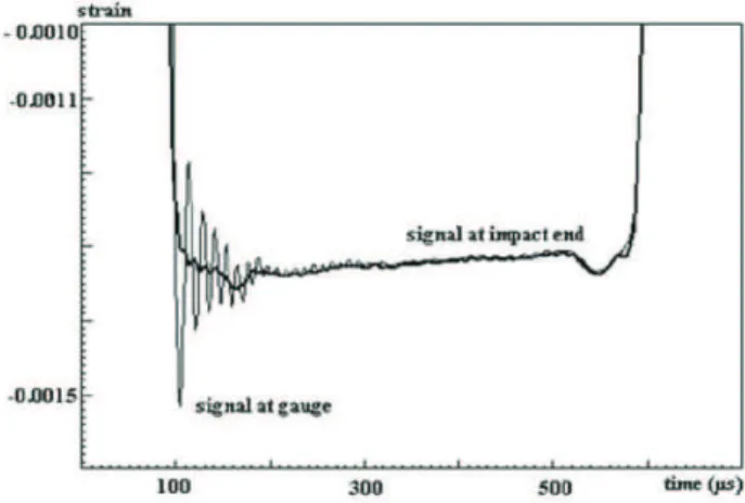
A good way to test the quality of the dispersion relation is to check whether the oscillations induced by the dispersion disappear at the impact side where the signal can be transported, as shown in fig. 5.

The two “ears” are due to two plastic rings used to guide the striker. (The non-nul slope is not explained)

Another way is to calculate the stress at a free end, which must be zero, as shown in fig. 6.

Fig. 5. Incident signal transported at striker side. (striker 1.3 m and input bar 3 m made of steel, diameter 20 mm. Incident gauge in the

middle, striker speed 13.3 m/s)

Fig. 6. The forces at a free end.

3.2 Case of visco-elastic bars

For viscoelastic bars, the argument ξ in equation (4) is a complex number so that a solution cannot be expressed in a simplified form such as (5). Consequently, the computation of the dispersion relation needs the functions λ∗

(ω) and µ∗

(ω) that describe the viscoelastic behaviour of the bars. The material properties of standard viscoelastic materials are often rep-resented with a rheological model. The simplest one (called Zenner model)

needs 3 parameters to be identified (first 3 left elements in figure 7). They could be identified in different ways, more often when dealing with bars by an inverse approach based on the measurement of the wave propa-gation on the bar itself. This is a safe method as, unlike for metals, material properties depend on various external factors.

Zhao and Gary (1995) have used an inverse method based on such an idea. They found that the Zenner model was not complete enough, and had to use a more complex model with 9 parameters (figure 7). Furthermore, following many authors, they assumed a constant Poisson’s ratio.

Fig. 7. A linear viscoelastic model

The same experimental set-up as in an impulse test is applied, where the waves are recorded at two different points in the bar. Using the wave at a recording point as input data, the parameters are determined in comparing the predicted wave and the recorded wave at another point (like in fig. 8)

It is also possible to avoid to solve equation (4). Dispersion may indeed be experimentally determined by comparing the wave Fourier components measured on two points on the rod – Blanc (1971), Lundberg and Blanc (1988), Gorham (1983), Bacon (1998). More recently, Hillstrm & al. (2000) developed a multi-point method using least squares. Another method, very accurate, is also proposed by Othman & al. (2001) based on a one-point measurement method using a spectral analysis of the resonant frequencies of the rod. An recent extension and improvement of this method proposed by Collet et al (2012) is presented in chapter 7.

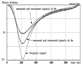
In order to illustrate the excellent quality of the dispersion relations generally obtained, an original record and two other records at respective distances of 4 m and 8 m of the original one, compared with their predictions, are shown in fig. 8.

By comparison with the elastic case (see fig. 4) it is observed that the dispersion correction is more important for common size viscoelastic bars and could not be neglected.

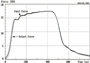
The importance of the correction in a real test situation is illustrated by showing both forces calculated in a test without specimen where the output force must obviously be equal to the input one (fig. 9 and 10).

Fig. 8. Test of the dispersion relation.

Fig. 9. Input and output forces without dipersion correction. For both viscoelastic and elastic bars, a precise dispersion correction does not suppress oscillations of the incident force in the case of sharp loading pulses. These oscillations are indeed the physical consequence of the wave dispersion.

At very high speeds of loading with short specimens, oscillations can also be seen in the output signal

Fig. 10. Input and output forces with dipersion correction.

3.3 Planerity of waves

The planarity of waves is extensively studied by Davies for the first mode. The solution of equation (4) is well known and illustrated in his paper for particular values of the frequency, as shown in figure 11 - from Davies (1948).

In this figure one sees, among other variables, the relative variation of the stress along the radius (xx/xx0). It shows that, at a relative high frequency

(in 19b, 0.935 corresponds to a non realistic value of the frequency for our standard steel bar: 280 kHz), the stress at the surface of the bar is negative when the average stress is positive. At a more realistic frequency (figure 19a – 94 kHz for our bar) one can see that the average stress is more or less 10% higher than the stress at the surface. The strain is not proportional to the strain, but those observations are also valid for the average strain. On has then to keep in mind that, depending on the frequency:

a) - The strain measured at the surface is not proportional to the average strain.

b) - The axial strain and the orthoradial strain are not proportional to each other.

c) - The axial stress is not proportional to the axial strain.

d) - The average axial speed is not proportional to the axial strain. Point (b) is well illustrated by Tyas and Watson (2001).

At lower frequencies, all the measurements become close to be propor-tional to each other.

A few authors – Safford (1992), Merle and Zhao (2006) have checked the validity of usual hypothesis commonly used. They proved that it is not worth taking care when frequencies f are under 2c/a (where a is the radius of the bar, equivalent for steel, to a/λ < 0.2 ). For the standard 20 mm steel bar, one observes that frequencies are in the good range.

4

Direct impact test

Recall here that, with non strictly 1 D bars.

The average strain is not proportional to the strain measured at the surface of the bar. The average stress is not proportional to the average strain

The dispersion of the waves induces significant changes in rising times of the signals.

The displacement at bar end is over estimated as the punching of the bar by the specimen is neglected (this point will be addressed later).

In the following, the basic understanding of SHB is recalled based on the 1-D propagation theory.

A convenient way to have a good understanding of waves propagation and reflections in a system of bars is to use the “Lagrange” representation together with formulas (2). In a space-time (abscissa-ordinate) diagram, the fact that the celerity of waves is constant induces that a wave event follows a straight line with an absolute slope c (figure 12).

Fig. 12. A typical Lagrange diagram. The two sloping lines show the path of the beginning and the end of a square signal in the space-time diagram. At a given point A, the time story show what could have been

recorded by a gauge at this point.

Direct impact test: 1 force and 1 displacement measurements. A force is applied at the end of a bar of length l starting at time t = 0. It produces a strain-time signal which is measured by a gauge at a (short) distance a of the bar end. The corresponding signal εi(t) starts at time

ts= a/c. The beginning of the signal reaches the other end (say output) of

the bar at a time te= l/c .

A given boundary condition is applied at the output end of the bar. In order to satisfy this (unknown) boundary condition, a new wave εr(t) in the

opposite direction is produced which starts at time te.

This reflected wave reaches point A at time tr= l/c + (l − a)/c.

From this time tr, the strain measured by the gauge is the sum of the

initial wave and of the unknown reflected one.

Consequently, the measurement duration based on the record of the ini-tial wave is ∆tm= tr− ts= 2(l − a)/c.

Say the strain measured at the gauge is εm(t).

The measurement duration is limited by the overlapping of waves. During this time∆tm,

The strain at bar (input) end is ε(t) = εm(t − a/c)

The force at input bar is F = E_bS_bε The speed at input bar is v = −cε

Fig. 13. A Lagrange diagram for an impact test. If

- one side of the specimen is fixed at the input end,

- the speed of the other side of the specimen can be measured, - the equilibrium of the specimen is assumed,

Then,

The force–(relative) displacement relation of the specimen can be com-puted.

5

SH(P)B. 2 forces and 2 displacements

measurements

The specimen is sandwiched between two bars. One force and one speed measurement are made on each bar-end in contact with the specimen. The output bars works as for the direct impact. It is not the case for the input bar where, due to the loading, there exists a wave prior to the loading of the specimen itself.

Torsion bars and direct tension bars will not be explicitly addressed here. Their analysis is based on the same knowledge of basic wave propagation theory, but they need to solve some specific technical problems concerning the loading of the system and the specimen clamping.

In this chapter, some problems related to the measurement side (that of forces and speeds) will be addressed. Anyway, due to the very common use of Kolsky’s formulas, this historical case is briefly recalled first, where problems dealing with the specimen behaviour have to be also introduced.

5.1 The special case of Kolsky bars

This very special case is interesting. For historical reasons, the gauges are equally distant from the specimen and both bars are identical. Considering the values of the strain at specimen ends, forces and displacements at both specimen ends are given by formulas (7,8)

vi= −cb(εi− εr) vo= −cb(εt) (8)

Fi= AbEb(εi+ εr) Fo= AbEbεt (9)

Where vi, vo, Fi, Fo are input and output speeds and input and output

forces at specimen faces, respectively. Ab, Eb, cb are area, Young’s modulus and celerity of waves in (identical) bars, respectively.

εi, εr, εt are incident, reflected and transmitted waves, respectively,

computed at specimen faces.

The measurement finishes here. In particular, the “Kolsky” formu-las that will be discussed later are resulting of more assumptions, mainly: identical bars and specimen equilibrium. This second assumption is always an approximation.

The situation is indeed here exactly the same as any measurement where the machine basically provides forces and displacements. Consequently it is possible, without any lost in the quality of measurements, to use different bars.

In Kolsky’s standard processing, the special assumption of equilibrium is used in the case of identical (same material, same diameter) bars. This yields - along with the superposition principle and formulas (7,8)- the well known relation:

εi(t) + εr(t) = εt(t) (10)

Consequently, assuming the homogeneity of stresses and strains within the specimen, the incident wave does not explicitly appear in the simplified formulas: εs(t) = ∫ t 0 ˙εs(τ )dτ = − 2cb ls ∫ 0 εr(τ )dτ σs(t) = Ab As Ebεt(t) (11)

where Asis the area of the specimen.

These simplified formulas are both based on equilibrium. When equi-librium is only badly verified, some researchers suggest the use an average formula for the stress (sometimes called the “three waves formula”). First, one must keep in mind that the average force could give a worth response than one of other input force or output force. Second, the simplified formula for the strain could also produce an imperfect result.

5.2 Overlapping of waves

The best way to address easily this problem is to make use of Lagrange diagram. It already has been seen for the direct impact test which corre-sponds, with the Kolsky apparatus, to the output bar. When equilibrium is not assumed and has to be checked, a measure of both input and output forces is needed. In this case, the best position for the input gauge appears to be in the middle of the input bar. Consequently the length of the output bar is such that the length between the gauge and its end is half of the input bar. If the bars do not have the same impedance, one must take care of propagation time and not of length.

Theoretically, the length of the striker could be as long as half of the input bar. In real situations one must account that the duration of the input wave is greater than that of the theoretical “square” one. The rising time of the signal has indeed to be added. For a given striker, this time is related to the imperfect geometrical matching of both striker and input bar ends. This mismatch can be due to imperfect surfacing and/or imperfect alignment but it can be considered equivalent to an imperfection of a constant thickness. A realistic interpretation of the rising time is that of the time needed for the bars to flatten the geometric mismatch.

In the case of a standard steel SHPB 20mm, the rising time is around 20µs with a striker speed of 10 m/s. It should be around 100µs at a striker speed of 2 m/s.

If the minimum loading speed is 2 m/s, these consideration lead to the standard optimal SHPB configuration, with:

Input bar length = 2l

Output bar length = l + 5d (5 diameters form the end for the gauge position)

Striker length = l -0.25 m (theoretical loading duration decreased by 100 s)

Note that for “pulse shaper” users, the rising time will increase and depend on the “pulse shaper” geometry and material.

In the case of viscoelastic bars and a viscoelastic striker, the analysis is a little different. With a striker and an input bar having the same impedance, the loading duration (in the 1-D analysis) is infinite, due to a tail. It is not easy to decide when the amplitude of the tail is small enough. It is then recommended, with viscoelastic strikers and bars, to use a striker with a smaller (by around 10%) diameter than the bars. Bussac et al. (2008) have indeed demonstrated that the incident pulse has, in this case, a finite duration.

5.3 Wave shifting. A precise method for SHPB.

The 1-D analysis of the waves implicitly takes account of the Saint-Venant principle: a certain distance is needed between the end of the bar and the strain gauge to insure the homogeneity of the strain across the bar (typically 5 diameters).

One needs then to use a wave theory to deduce the strain (as it would be is this point was not an end) at the end a bar. This operation is called shifting.

It is clear that the input force is proportional to the sum of the incident and reflected waves and that a relative imperfect shifting in time would induce an error, especially at the beginning of the loading. Some authors have proposed to use some geometrical trick at the beginning of the signals to define a “foot” for the curves and determine the shifting process on the knowledge of these points: we call that the “foot shifting” technique. Acceptable results could be obtained for the input force, with this method. If we extend the method to the output wave, it induces a wrong evalu-ation, at least, of the strain, if it neglects the times needed by the loading to go across the specimen.

The shifting process must then be precise. A method, introduced by Zhao & Gary (1996),can be used. It is based on the transient simulation of an initial elastic behaviour of the specimen. The method also allows for a correction of specimen geometry and a measurement of the Young’s modulus of the specimen material.

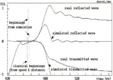
The incident wave at the input specimen face been known (after the shift-ing process), reflected and transmitted waves can be computed – dependshift-ing on specimen dimensions, bar dimensions and mechanical properties, speci-men Young’s modulus. The only unknown is the last one. Using a try and error method, one rapidly finds the Young’s modulus that gives shapes of both simulated waves similar to that of transmitted and reflected waves as they are known (after the shifting process) at the input and output specimen faces.

Note that this operation does not work if the dispersion is not taken into account, even with elastic bars. The reason is that the elastic response of the specimen concerns the first instants of the loading where the initial slope is strongly affected by the dispersion.

Some distance in time is still often observed between real and simulated waves. This distance can be due to an imperfect knowledge of the speed of waves or, more often, to some geometrical imperfection of the specimen. For an optimized stress-strain curve, real waves are shifted to simulated ones. This very short shift (equivalent of a few cm in distance) is not affected by the dispersion. An illustration of the method is presented in figures 14 and

15.

Fig. 14. Optimal choice of Young’s modulus for transmitted and reflected waves.

The precise way stress and strain are computed will be addressed later. Remind that the best results are derived from the force and displacement time histories at the specimen boundaries without artificial time shifts.

Fig. 15. an example of possible effect of the method. Case of a concrete specimen.

Recall that the method does not work correctly without the dispersion correction and that it relies on an initial non negligible elastic behaviour of the specimen.

It still perfectly works with (slightly) viscoelastic bars (as Nylon or PMMA bars) but not with a purely viscous specimen.

5.4 Punching of the bar-end by the specimen

After using this method during years, we have observed that the expected modulus of the specimen was found when the specimen diameter was close to that of the bars. The measured value was lower than the expected one in most situations when the specimen diameter was smaller than that of the bars. Furthermore, for a given specimen diameter, the discrepancy was decreasing with specimen length.

This problem, due to the local punching of the bar end by the specimen, has been addressed by Safa & Gary (2010). They have shown that this effect is like that of an added spring at the end of the bars: the displacement due to punching is proportional to the applied (and measured) force. A simple formula has been established that gives the value of the displacement due to punching. Results are summarised in figure 16 next page.

Note that the 1-D elastic behaviour of punching allows for taking ac-count of its contribution in the elastic simulation process. Consequently, the Young’s modulus of any material specimen can be directly estimated by means of the elastic simulation process.

It is clear that the relative influence of the displacement due to punching increases when the length of the specimen decreases. This is especially important at high or very high strain-rates that need shorter specimen (as the incident striker-speed is limited by the care of the gauges) when the specimen diameter is under the half of that of the bar.

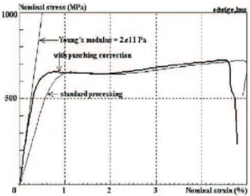
For a real test made at 10000/s, with a specimen metricconverterPro-ductID3 mm3 mm thick, diameter 6.5mm (steel bars, 12 mm, striker speed 25m/s), the equivalent in strain due to punching, at the plastic plateau, is around 14%. On the other side, at low strain rates, when the total mea-sured strain is small, the effect of punching is still important as illustrated in figure 17.

Fig. 17. Influence of the punching correction. (20 mm steel bar, striker speed 2.79 m/s, strain-rate around 100/s).

5.5 Force matching. Critical case of the input side.

This problem has nothing to do with a so called “impedance matching” problem (discussed later).

In most cases, especially when testing metallic specimens, input and output forces are almost equal. This is not always the case, as shown later. Anyway, in the following analysis, we use this assumption to make clearer the ”force matching” problem.

Considering formula (9), it appears that a correct measurement of the output force is only possible when the measured output strain is itself sig-nificant. It can be considered that strain measurements are done with a precision around 5.10−6 _{when using classical strain-gauges. With}

semicon-ductor gauges, it can be improved by a factor 50. Considering that an acceptable relative precision of 2% is suitable for any measurement, the maximum strain measured should be more than 2,5.10−4_{. Using formula}

(9) allows for the calculation of the minimum suitable output force. In the example of a steel bar (20 mm diameter), this force is around 15 kN. The specimen area being at maximum equal to the bar diameter, the corresponding stress is 50 MPa. For weaker materials, it is necessary to use semiconductor gauges or a better amplifying system (or a bar with a low Young’s modulus, as it is the case of most viscoelastic bars).

Let us then assume that a material, with a maximum stress of 50 MPa, is tested with the steel bar, very carefully. Considering now formula (9) for

the input force, it appears that a precise measurement is not possible when the amplitude of the incident wave and the opposite of the amplitude of the reflected wave are too close.

Keeping this example, if we wish to obtain high strain rates, we use a small specimen length. For sake of simplicity, we assume that the tested material is not strongly rate sensitive. A simple simulation, with a specimen 5 mm long, shows that the striker speed must be 15 m/s to obtain an average strain rate close to 3000/s. In this case, the absolute amplitude of the reflected wave only differs by 15% from the amplitude of the incident wave. A precise calculation of the input force with formula (9) is then difficult.

If we consider that an acceptable result is obtained when both waves differ by more than 20%, the maximum strain rate giving an acceptable result is, for this example, around 400/s. It can be concluded that materials with a plateau stress under 50 MPa cannot be safely tested with 20 mm steel bars at strain-rates over 400/s.

More generally speaking, weak materials need the use of soft bars. This problem should be called the “force-matching” problem as it has nothing to do with the specimen impedance, but only with the product of the Young’s modulus of the bar by its area to be compared with the maximum force to be measured.

Optimizing specimen dimensions. In order to insure good mea-surements on the input side (more often of the force) the specimen has to be design depending on the required strain-rate.The problem is also to choose the appropriate striker speed to obtain the strain rate. One can use a method presented by CityplaceGary (2001), which is based on simple assumptions (one-dimensional wave analysis, specimen equilibrium, evalua-tion of the material stress: say σy). The amplitude of the incident wave is

deduced from the striker speed V (eq. 11a). The amplitude of the transmit-ted wave is deduced from the specimen section Ssand σy (eq. 11b), and the

amplitude of the reflected wave is deduced from the equilibrium (eq. 11c). εi=_2cV (11a), εt= _SSs_bσ_Ey_b (11b),

εr= −εi+ εt(11c), ˙εs= 2cε_lsr (11d)

where Sb and Eb are the section and the Young’s modulus of the bars, respectively.

The average strain rate is now given by formula (11d), where c is the wave speed in the bars and ls is the specimen length. It is then possible to make sure that the relative amplitude of the reflected wave is small enough in comparison with the relative amplitude of the incident wave. If we look at formulas (8) and (9), it can be seen that the best situation, i.e., that giving the most accurate force and speed results, is that occurring when the amplitudes of the transmitted and reflected waves are fairly similar.

These formulas make it possible to easily determine optimized specimen dimensions and striker speeds.

5.6 Impedance matching

The impedance matching problem, has been addressed by Davies and Hunter (1963). It mainly deals with the homogeneity of stresses and strains in the specimen, during a Hopkinson bar test, and especially at early in-stants.

During this loading phase, input and output forces are alternatively bigger than the other. An example is shown in fig 18, from Klepaczko (2007) -figure 3.11a, p 206.The gap between both forces decreases when the speed of waves in the specimen increases and when its length decreases. It also decreases when the amplitude in force (in stress in the present figure) of the first step decreases.

Here is the “impedance” matching problem that describes the conditions to make this step small enough. Furthermore, this step is softened if the rising time of the loading is increased. This point is one reason for using pulse shapers.

Fig. 18. Elastic input and output stresses at early instant of the loading -from Klepaczko (2007).

5.7 Holding the specimen: dealing with one-point measurements Measurements with bars are always analyzed within the 1-D hypothesis (even with dispersion and punching corrections as both are only expressed as a function of the axial coordinate of the bar). In other words, force and speed measurements, on each side, are made at a single point. This basic hypothesis does not appear when Kolsky’s formulas are used for a direct stress-strain relation. It is then important to keep in mind this aspect, especially in situations where holding the specimen leads to the use of devices that induce an impedance change along the wave propagation path.

Some examples are given here.

When compression bars are used to test a material specimen, the spec-imen diameter must be smaller than the diameter of the bar to ensure a quasi-uniaxial state of stress. When very weak material are tested, even with viscoelastic bars, the quality of the measurement is limited by force matching problems described above.

In order to overcome this limitation, one could use at bar ends a device with a larger diameter and then be able to hold a specimen with a much larger specimen. Such a technique is illustrated in figures 19 and 20.

Fig. 19. Impedance change between the bar (tube) and the specimen.

Fig. 20. Special device for a larger specimen.

The first question here is to decide at which point is made the measure-ment: end of the bar or specimen face?

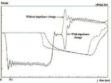
In order to illustrate this problem, a brass specimen has been tested in the situation shown in fig. 20 and in a classical situation with the same (aluminium) bars. The corresponding recorded waves are shown in fig. 21

Fig. 21. Illustration of the influence of a matching device – waves. It is observed that the strongest influence appears in the reflected wave, and that the transmitted wave is smoothed (this is not a general results as it

depends on each impedance ratio device/bar).

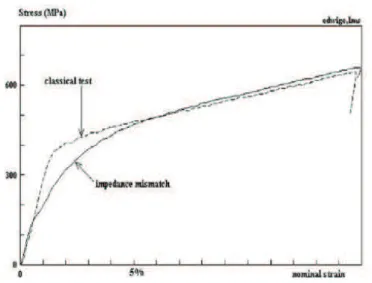
A standard processing of the waves will then give wrong results when matching devices are used, as shown in figures 22 and 23.

Fig. 23. Apparent stress-strain relation with and without devices.

Looking at the stress-strain diagram shows a difference that is not so large, in particular for larger strains. The main effect is a smoothing of the stress-strain relation that prevents for an acceptable evaluation of the elastic limit of the tested material.

When it is not possible to avoid the use of a matching device, an impedance correction is possible. A simple way is to use a one dimensional analysis. Knowing the waves at the end of the bar (in the part with a constant impedance), the waves at specimen faces can be calculated, assuming the 1-D elastic behaviour of the devices of known impedance. The forces and the displacements applied to the specimen faces are then deduced.

5.8 Undetermined specimen ends

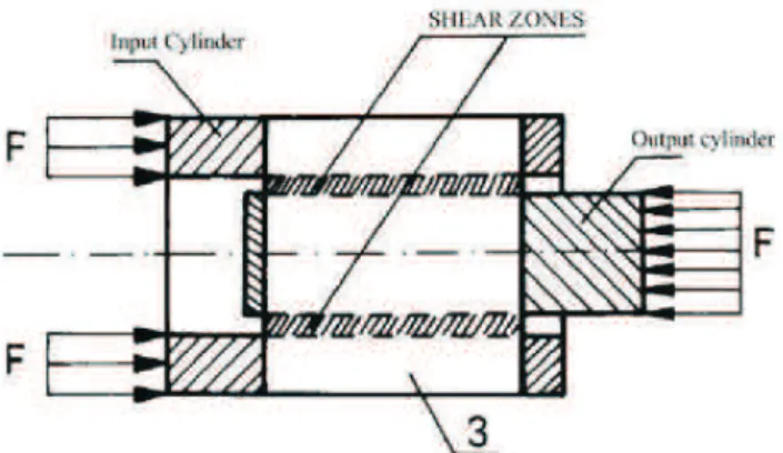
A good example is found in a work of Gary and Nowacki (1994). They proposed a device to convert compression in shear. The idea is summarised in fig. 24.

The (say) input hollow cylinder has the same impedance than the input bar when the output cylinder has the same impedance as the output bar. The problem here is that the beginning and the end of the specimen are not defined. Consequently one has to consider that the shear-displacement curve is filtered with a cut-off frequency depending on the length of the shear zone.

Fig. 24. Conversion compression to shear.

6

Specimen behaviour

The Split Hopkinson pressure bar arrangement can give very accurate mea-surements of forces and velocities at both sample faces if the data process-ing is carefully performed. Relatprocess-ing material properties to measurements of forces and velocities at the two specimen faces is a completely independent problem.

For this reason, we have distinguished the problems of measuring ac-curacy of SHPB and material property identification from the measured data.

6.1 Axial homogeneity

Due to the presence of waves in dynamic experiments, both the stress and strain fields within a specimen are seldom uniform. A dynamic material test should be designed such as to minimize this inherent non-uniformity, a condition which is typically associated with “quasi-static equilibrium”. However, when testing purely elastic materials such as fiber reinforced com-posites or low impedance materials, the validity of this assumption needs to be checked with care. Note that there are situations where force equilibrium can exist without strain homogeneity as it is often the case with structural materials like honey-comb or foam.

Before computers became generally available, the assumption of quasi-static equilibrium of the specimen had a special importance from a data processing point of view.

The idea was to associate, in a “memory scope” (the image was stored in an analogic way) the “strain” and the “stress” signals and directly observe a curve proportional to the stress-strain curve of the material. First, the strain-rate was analogically integrated with respect to time. Then, the simplest way to synchronize both signals was to produce them at the same time. This was the reason to use both bars of same length with each gauge in the middle.

With the use of modern numerical acquisition, the output gage can now be positioned closer to the specimen interface; consequently, the output bar can be shorter than the input one (and there is no good reason to choose its length equal to that of the input bar). The use of “equilibrium” condition was also crucial at that time as the input force could not be directly measured.

Optimal design with equilibrium. It is worth noting here that this equilibrium condition could be used with different input and output bars leading to slightly more complex formulas. In the same way, other formulas could be derived using any pair of waves (among three).

Let’s consider the idea of using only the incident and transmitted waves. For sake of simplicity we suppose that the two bars are still identical but the results could be generalized to a SHPB made of two different bars. Assuming equilibrium, formula 3 can also be written:

εs(t) = ∫ t 0 ˙εs(τ )dτ = − 2cb ls ∫ 0 (εi(τ ) − εt(τ ))dτ σs(t) = Ab As Ebεt(t)

where Ab is the area of the bar, Ebits Young’s modulus and Asthe area of

the specimen.

It can be seen that only the incident and the transmitted waves are now involved in the processing formulas. Finding an optimal position for the gauges, close to the input side of the bars where the waves arrive first, (see the case of direct impact) will then lead to an increased measured strain. It is then easy to find the optimal design close to the one shown in figure 25. The bars have now to have the same length to allow for the same duration of the incident and the transmitted waves. Consequently, the striker has to be as long (or longer) as the remaining distance between the gauges and the end of the bars.

Fig. 25. With equilibrium, a configuration for an increased duration measurement.

Evaluation of specimen behaviour. The evidence of non equilibrium is found in early instants of the loading, when the first wave in the specimen has not yet reached its end. At this instant the input force exists when the output force is still null. Knowing that specimen equilibrium is never achieved exactly, we seek the best of the commonly used stress-strain curve estimates in a SHPB experiment. This question is studied by Mohr et al. (2010). The time shift of the waves is found to play a critical role as far as the accuracy is concerned.

More specifically, it is found that the omission of artificial time shifts (as illustrated in fig 26) provides the best stress-strain curve estimates. In other words, once the force and displacement histories are known at the specimen boundaries, accurate estimates of the stress-strain curves should be made without further shifting the signals on the time axis.

Fig. 26. Exact theoretical waves as shifted at specimen faces. The dashed blue line shows the strain history of the transmitted wave after shifting the beginning of this wave in time (so-called “foot shifting”) such that all

strain histories begin simultaneously.

Estimations evaluated by Mohr et al. (2010) are based on exact explicit calculation done in the frequency domain. Results confirm that the error (for all formulas) increase with the impedance mismatch between the spec-imen and the bars. It is emphasized that, in standard testing situations, exact shifting (illustrated in fig 26) is much more important than strain or force approximation (with 2 or 3 waves).

Fig. 27. Plot of the estimated stress strain curves for a dynamic compression experiment on PMMA (steel bars

metricconverterProductID20 mm20 mm).

The estimates which are based on the force and displacement time his-tories at the specimen boundaries without artificial time shifts, provide the most accurate stress-strain curve. Unless accurate input force measurements are available, the combination of the average strain with the output force based stress estimate is recommended for standard SHPB experiments. An illustration is given in fig. 27.

Recall that in the elastic range and in standard SHPB testing, when the specimen diameter is smaller than half of that of the bars, the incidence

of the punching correction on the quality of the results is the most important.

6.2 Radial homogeneity. Friction and inertia

We must keep in mind that, alike in all testing situations, axial stress and strain homogeneity (considered up to now) is not the only one to be considered. In quasi-static testing, it is possible to directly measure the strain in a “gauge section” of the specimen where 1-D assumptions are well verified. In SHPB, when using a cylindrical specimen, it is more difficult to avoid friction at specimen faces. This friction prevents the expected radial expansion quantified by Poisson’s ratio.

The consequence is that the triaxial stress-state is not uniform along the axial loading. It induces an average over-stress in the common situation of elastoplastic materials.

This radial expansion is also prevented by inertia effects that induce lateral confinement.

An empirical formula has been established by Malinowski and Klepaczko, (1986) that takes account of both effects. This formula is valid for purely plastic materials but gives a first order correction that applies to many other materials. σ − σ0= µσ 3s + ρd2 12(s 2₋ 3 16)( ˙ε 2_{+ ¨ε) +}3ρd2 64 ε¨ where, σ0 : ideal value, σ : actual value (true stresses)

land dactual values of length and specimen diameter and s = l/d ρ , density assumed to be constant

µ friction Coulomb coefficient (usually <0.1).

This formula indicates that the inertia effect is much smaller than that of friction for common metal testing (bar diameter < 20 mm). It becomes significant for bigger specimens (>30mm) like found for rock or concrete testing when big specimen sizes are required for a good average material representation. It is seen in this case that some artificial strain rate effects can be attributed to bi-axial loading induced by inertial confinement.

In the case of testing where a quasistatic radial confinement is added -see Gary and Bailly (1998), and Forquin et al. (2010) - inertia effects are prevented and do not operate anymore.

6.3 Adiabatic heating

The duration of a dynamic compression test with SHPB is almost always under 1 ms. For many materials, it induces large strains (depending on strain-rate) that produce work which is (partly ?) converted into heat. In

case of metal or polymer testing, it can induce a specimen temperature increase in the range up to 100◦

C.

It is then important to account for this temperature increase for an improved evaluation of the material behaviour. This question has been in-vestigated by various authors who have proposed techniques for high speed temperature measurements (more often based on infrared specimen emis-sion). See for instance Rittel (1999) and Negreanu et al. (2009).

6.4 Inverse methods

On the basis of force and velocities measurements at specimen faces, an approach of the specimen behaviour based on an inverse method is theo-retically possible, as shown by Rota (1994), as these four values are super-abundant measurements.

3-D dynamic numerical simulation could allow, in this case, accounting for friction, radial inertia and possibly temperature increase. If an appropri-ate form of the mappropri-aterial behaviour with some parameters to be determined is known, using a part of data (two velocities, for example) as the input data, another part of data (the two forces) associated with the given parameters can be calculated. The best set of parameter which gives the calculated forces well in agreement with the measured ones can theoretically be found. In order to further investigate this approach, we shall limit the analysis to axial 1-D effects by means of a fast 1-D transient simulation based on the Sokolovsky (1948) and Malvern (1951) approach.

The uniaxial governing equation and the constitutive law are written in equations (12) ∂σ(x,t) ∂x = ρ ∂v(x,t) ∂t ∂ε(x,t) ∂t = ∂v(x,t) ∂x (12) f (σ, ε, ˙σ, ˙ε, ...) = 0

where σ, ε, v are the stress, the strain, and the particle velocity in the spec-imen. ρ is the mass density.

The boundary conditions at the two faces of the specimen are given as follows:

σ(x, t) − EBSB CBSS

v(x,t) = 2SB SS

EBεi(t) at the input side

σ(x, t) + EBSB CBSS

EB, CB, SB, Ss denote the Young’s modulus, wave velocity, cross-sectional

area of the bar and the section of the specimen.

Once the specimen behaviour is assumed, the direct problem described by equations (12, 13) corresponds to an uni-dimensional SHPB simulation. As mentioned above, the simulation would be just the preliminary stage of the inverse problem which consists in finding the parameters of the model. The inverse methods need fast calculation procedures to allow for a great number of direct calculations with different sets of parameters if necessary. For this purpose, the specimen behaviour should be numerically easy to calculate. This is why it is chosen to use a Sokolovsky-Malvern model type for the specimen, (14).

∂ε ∂t = 1 E ∂σ ∂t if σ ≤ σs ∂ε ∂t = 1 E ∂σ ∂t + g(σ, ε) if σ > σs (14) The characteristic network in this case is composed of families of straight lines so that the numerical integration of equation (13, 14) by the method of characteristics is very efficient. In comparing the given behaviour with the average stress strain curve obtained from three simulated waves, the efficiency of classical SHPB analysis for this type of materials can be eval-uated.

It is noted that the Sokolovsky-Malvern constitutive model is a quite general rate-sensitive one. Though it has been introduced initially for met-als, it can be also used to describe the non-metallic materials if the function g(σ, ε) is correctly chosen –see Critescu (1967).

In order to have a general idea of the efficiency of the classical SHPB analysis for this type of constitutive models, a popular rheological model (Fig. 28) is examined here, which is of Sokolovsky-Malvern type with the g(σ, ε) expressed as follows,

g(σ, ε) = (1 +

Ev

E)σ − Evε

Fig. 28. Rheological model for 1-D standard elasto-visco-plasticity.

A number of simulations were done for different sets of parameters. It has been found, like for previous results on metals, that the classical average stress-strain curve is in good agreement with the curve given by SHPB standard analysis at relative important strains. However, in the range of small strains, it is acceptable when the viscosity is low even if there is no axial uniformity. On the other hand, when the viscosity is high, the average (SHPB) curve is quite far from the given behaviour.

Fig. 30Simulated and measured forces for concrete.

An illustration of the method is presented in two particular cases: for salt in fig. (29) which exhibits a strong viscoplastic behaviour and for concrete fig. (30) which breaks, showing a negative strain hardening, at small strains. In both cases, equilibrium conditions are obviously not satisfied.

The chosen model with the set of parameters which gives the best agree-ment can be considered as a representative model of the specimen in this test. As a result, the stress and strain fields in the specimen are evaluated so that a stress-strain curve is found. The assumption on the uniformity of stress and strain fields is then not needed in such a method. The only hypothesis used is that specimen tested manifests the same properties every-where. Furthermore, it is possible to give a stress strain curve at a constant strain rate via the model and the set of parameters identified.

This stress-strain curve can then be compared with the one obtained with the classical SHPB analysis. For the test on salt, the two curves are quite far from each other in the range of small strains. The inverse calculation is then in this case the only way to obtain an accurate result for this type of materials. On the other hand, for the test of concrete, the average stress-strain curve is rather close to the curve derived from the model, as a kind of averaging operates between input and output forces. The inverse calculation could then be avoided.

7

Measurement of the dispersion relations

A method is briefly presented here that provides a very accurate estimation of the dispersion relations. One reason is that it is a one point method; the other is that it is based on simple formulas and an easy identification of the wave speed and damping at a given finite set of frequencies.

Furthermore, it allows for a subsequent mathematical analysis which includes noise reduction and provides a rheological model with a number of elements that is in accordance with the complexity of the material.

7.1 Impact test method. Theory

Fig. 31Impact test with a uniform viscoelastic bar specimen. At one end, x=0, the bar is impacted axially by a striker that separates from the bar after the generation of a compressive primary pulse in the bar. The other end of the bar, x = l, is free. The strain εb(t) = ε (b, t)

is recorded at a distance a from the free end and b from the impacted end (a + b = l). The primary pulse should be shorter than 2a so that there is no overlap in the measured strain of this pulse and the first pulse reflected from the free end. However, it should be much longer than the diameter of the bar so that approximate 1D conditions prevail - Hillstrm et al (2000).

In the frequency domain, the strain in the bar can be expressed as: ˆ

ε (x, ω) = A (ω) e−iξ(ω) x_{+ B (ω) e}iξ(ω) x_{, (16)}

where

ξ2_{(ω) = ρω}2_{/E(ω), ξ (ω) = k (ω) − iα (ω) (17)}

Here, ˆε (x, ω) is the Fourier transform of ε (x, t), and A (ω) and B (ω) are complex amplitudes of waves travelling in the directions of increasing and decreasing x, respectively, k (ω) is the wave number and α (ω) is the damping coefficient.

In order to determine an expression for the recorded strain ˆε1 b(ω) =

ˆ

first determined from Eq. (16) and the boundary conditions ˆε (0, ω) = ˆε0(ω)

and B (ω) = 0 for a semi-infinite bar x ≥ 0 , where ˆε0(ω) is the strain at the

impacted end. With these amplitudes and x = b inserted, Eq. (16) gives ˆ

ε1b(ω) = e −iξ b_εˆ

0(ω) (18)

The recorded strain ˆε1

b(ω) = ˆε (b, ω) associated with the complete train

of pulses is determined similarly. With amplitudes A and B, and x = b and l − b = a inserted, Eq. (16) gives

ˆ ε∞

b (ω) =

sin (ξa)

sin (ξl)εˆ0(ω) . (19) Dividing the members of Eq. (19) by those of Eq. (18) eliminates the strain ˆε0(ω) at the impacted end which normally cannot be measured. The

elimination of this strain makes the difference between the method used here and that used by Othman et al. (2001). Substituting ξ from the second of Eqs. (17) into the result, one gets the ratio ˆε∞

b (ω) /ˆε1b(ω) which gives |ˆε∞ b (ω)| 2 = ˆε1b(ω)   2 e2α bsin 2_{(ka) + sinh}2 (αa) sin2(kl) + sinh2(αl). (20) Resonance occurs at the angular frequencies ω = ωm, m=1, 2,. . . which

correspond to the wave numbers, wavelengths and phase velocities

km= mπ l , λm= 2π km = 2l m, cm= ωm km = ωml mπ, (21) respectively.

It is assumed that within the m:th resonance peak α = αmω/ωmcan be

taken as directly proportional to angular frequency and c (ω) = ω/k (ω) = cm can be taken as constant. By use of the third of Eqs. (21) we then

obtain the relation between wave number and angular frequency within the resonance peak. Inserting these expressions for α (ω) and k (ω) into Eq. (20) we get (m = 1, 2, . . . ) |ˆε∞ b (ω)| 2 = ˆε1b(ω)   2 e2αmbω/ωmsin 2_(k

maω/ωm) + sinh2(αmaω/ωm)

sin2(kmlω/ωm) + sinh2(αmlω/ωm)

(22)

within the m:th resonance peak. In this relation, the spectra |ˆε∞ b (ω)| 2 and ˆε1 b(ω)   2

can be determined experimentally.

For each resonance m=1,2,. . . , the resonance frequency ωmand damping

resonance peaks represented by the left and right members of Eq. (16). From ωmand m, the complex modulus Emat each resonance frequency can

be finally obtained as Em= ρ ( ωm ξm )2 , ξm= mπ l − iαm, m = 1, 2, . . . . 7.2 Experimental set-up and procedure

Impact tests were carried out with a Nylon bar specimen of length 3045 mm, diameter 10.2 mm, and density 1149 kg/m. The striker had length 174 mm and the same diameter 10.2 mm and material as the bar, and its impact velocity was 3.7 m/s. The strain was recorded with 500 kHz sampling frequency, and the signal vanished completely before the end of the recording window (fig. 32 and 33)

Fig. 32Recorded strain in the Nylon bar specimen. Long-time record of strain pulses.

Fig. 33Primary strain pulse followed by strain pulses which have undergone one and two free-end reflections

The spectrum |ˆε∞

b |, computed from the long-time strain record, is shown

in Fig. 34, 35 and 36. It is easily checked that resonance peaks are clearly identified. In figures 35 and 36, the experimental peak is shown with the theoretical one identified by the minimization process described above (in figure 35, the superposition is perfect at the scale of the drawing).

Fig. 35Spectrum, zoom on f=270 Hz

Fig. 36Spectrum, zoom on f=6860 Hz

Corresponding to the peaks, a set of experimental points is obtained which provides, for each frequency, a value for wave speed and damping (circles in figures 37, 38)

Fig. 37Wave speed

Fig. 38Damping

By averaging, the results in figures 37 and 38 immediately provide the dispersion relations that could be used right away for the wave shifting.

Using the mathematical analysis presented by Collet et al. (2012), an optimal rheological model type is built and identified with 7 springs and dashpots. Note that the number of elements is not an assumption - as was done in Othman et al. (2001) - but is a result of the method. Knowing the

corresponding Young’s modulus, wave speed and damping as functions of frequency are then built. In the present example, they correspond to black continuous curves in figures 37 and 38.

8

Long-time measurements

Basic measuring techniques involving the use of bars require the knowledge of the two elementary waves which propagate in opposite directions. Once they have been characterised, they can be shifted to the appropriate cross-sections (the bar specimen interfaces for example) and all the mechanical values required can be calculated. The SHPB technique involves the inde-pendent measurement of each wave.

Some authors - Lundberg & Henchoz (1977), Yanagihara (1978), Zhao & Gary (1997), Jacquelin & Hamelin (2001) - have carried out two measure-ments on each bar. The pioneers in this respect were Lundberg & Henchoz (1977) and Yanagihara (1978), who independently developed a wave sepa-ration technique based on one-dimensional wave propagation theory. Their methods didn’t take into account the wave dispersion. Some attempts have been made to develop methods also accounting for the wave dispersion, starting with Zhao & Gary (1997). However, the solutions proposed so far are sensitive to noise. A wave separation technique based on multiple measurements has been proposed by Othman & al. (2001) and Bussac & al. (2002). In line with Jacquelin and Hamelin (2003), this method will be subsequently called the BCGO method. It is based on the Maximum Likelihood approach and involves performing multiple strain measurements on each bar. This method, which is not noise-sensitive, requires an extra velocity measurement at very low strain rates. Jacquelin & Hamelin (2003) have developed an alternative three-point wave separation technique which is also insensitive to noise but the gauges are cemented to specific points and the force is calculated at one bar end (which is the only point where it can be calculated). The BCGO method is illustrated with the analysis of Split Hopkinson Bar tests, and an extended range of strain-rates (from 10−1 _{to 5 10}3 _{s-1) for the study the rate sensitivity of an aluminum alloy.}

8.1 Wave separation: the BCGO method

In this section, the BCGO method is briefly presented.

Let us consider an elastic or viscoelastic bar with length l. In the case of single mode propagating longitudinal waves, the stress, strain, displacement and velocity are expressed in terms of the Fourier transforms as follows:

˜ ε (x, ω) = A (ω) e−iξ(ω)x_{+ B (ω) e}iξ(ω)x ˜ σ (x, ω) = E∗ (ω) (A (ω) e−iξ(ω)x_{+ B (ω) e}iξ(ω)x) ˜ v (x, ω) = −ω(A (ω) e−iξ(ω)x_{− B (ω) e}iξ(ω)x) /_{ξ (ω)} ˜ u (x, ω) = i(A (ω) e−iξ(ω)x_{− B (ω) e}iξ(ω)x) /_{ξ (ω) (23)}

where A (ω) and B (ω) are the Fourier components of the forward and downward waves, respectively, at the origin of the bar, E ∗(ω) is the complex Young’s modulus and ξ (ω) = k (ω) + iα (ω) is the complex wave number. Eqs. (23) show that the strain, stress, displacement and particle velocity can be obtained at any point on the bar if the following four parameters are known: ξ (ω) , E∗

(ω) , A (ω) and B (ω).

The two parameters E ∗ (ω) and ξ (ω) depend only on the bar character-istics (its geometry and material). They only need to be determined once. Here we used the method presented in chapter 7.

In what follows, E ∗ (ω) and ξ (ω) are therefore assumed to be known. A(ω) and B (ω) are calculated based on the data obtained by performing three strain measurements and one velocity measurement. We express the fact that the signals recorded are noisy by writing that they are the sum of the exact value of the strain (or the velocity) and an unknown noise. The statistical distribution of the noise is assumed to be Gaussian. Conse-quently, the Maximum Likelihood Method can be used to estimate the two functions A(ω) and B (ω). This consists in writing that the signals measured correspond to the most probable event. Our problem is therefore equivalent to the minimization of a functional: this minimization yields an explicit formula for A(ω) and B (ω) as a function of the material and geometric parameters and the measured quantities - see Bussac & al. (2002).

The elementary functions A(ω) and B (ω) are then computed for each test. Using eqs. (23), one can now determine the force and the velocity at each point on the bar, especially at the bar ends. By applying the BCGO method to each of the bars, it is then possible to assess the force and the velocity at the two bar/specimen interfaces.

8.2 Experimental set-up

As an example, it is proposed to explore the strain-rate sensitivity of aluminium. The behaviour of this material is explored under a large range of strain rate conditions: quasi-static, medium and high strain rates.