Continuum damage modelling in geomechanics

HAL Id: hal-01570542

https://hal.archives-ouvertes.fr/hal-01570542 Submitted on 31 Jul 2017

HAL is a multi-disciplinary open access archive for the deposit and dissemination of sci-entific research documents, whether they are pub-lished or not. The documents may come from teaching and research institutions in France or abroad, or from public or private research centers.

L’archive ouverte pluridisciplinaire HAL, est destinée au dépôt et à la diffusion de documents scientifiques de niveau recherche, publiés ou non, émanant des établissements d’enseignement et de recherche français ou étrangers, des laboratoires publics ou privés.

Continuum damage modelling in geomechanics

Gilles Pijaudier-Cabot, Ludovic Jason, Antonio Huerta, Jean-François Dubé

To cite this version:

Gilles Pijaudier-Cabot, Ludovic Jason, Antonio Huerta, Jean-François Dubé. Continuum damage modelling in geomechanics. Felix Darve, Ioannis Vardoulakis. Degradations and Instabilities in Ge-omaterials, 461, Springer, pp.77-105, 2004, International Centre for Mechanical Sciences book series (CISM), 978-3-211-21936-2. �10.1007/978-3-7091-2768-1_3�. �hal-01570542�

Continuum damage modelling in geomechanics

Gilles Pijaudier-Cabot1, Ludovic Jason1*, Antonio Huerta2,and Jean-Fran9ois Dube3 1

R&DO- GeM, Ecole Centrale de Nantes, France

2

Laboratori de Calcul Numeric, Universitat Politecnica de Catalunya, Barcelona, Spain 3

LMGC/UMR5508, Universite de Montpellier II, France *also at EDF R&D, Clamart, France

Abstract: _{Continuum damage mechanics is a framework for describing the variations of} the elastic properties of a material due to microstructural degradations. This chapter presents the application of this theory to the modelling of concrete. Several constitutive relations are devised, including incremental, explicit, and non local damage models. A general framework for damage induced anisotropy is also presented. Coupled damage and plasticity modelling is discussed. Finally, the issue of the experimental determination of the internal length in non local models is tackled.

3.1 Introduction

This chapter is concerned with the presentation of several continuum damage models and their implementation in non linear finite element analyses. Continuum damage means that the mechanical effects of progressive microcracking, void nucleation and growth are represented by a set of state variables which act on the elastic and/or plastic behaviour of the material at the macroscopic level. First, we will deal with the scalar damage model and present different versions of this type of constitutive relations. After having recalled how the local integration of the constitutive relation can be performed in the same spirit as for plasticity-based models, we will deal with more specific applications: cases where the evolution of damage is specified in an integrated form, where damage induced inelastic strains are introduced, wheye crack closure effects are modelled, and finally where damage is coupled to plasticity. The following section deals with damage induced anisotropy. A general framework for capturing directionality of damage is recalled. Coupling with plasticity and crack closure effects are also discussed. Non local damage is developed in the fourth section. We present integral and gradient models. In particular, a general scheme for the implementation of the gradient model, implemented into the finite element code "Code_ Aster", is described. The fifth section deals with several computational issues related to damage such as the implementation of the model within secant or tangent algorithms. The chapter concludes on the problem of the calibration of the model parameters in damage models including the internal length. Inverse analysis of

3.2 Isotropic Damage Model

When damage is assumed to be isotropic, it is considered that it produces a degradation of the elastic stiffness of the material through a variation of the Young's modulus:

(1)

where v_{0 ,} E₀ and ~J are the Poisson's ratio and Young's modulus of the undamaged isotropic material and the Kronecker symbol respectively. The elastic (i.e. free) energy per unit mass of material is:

(2)

where C0 is the stiffness tensor of the undamaged material. This energy is assumed to be the state potential. The damage energy release rate is defined as the variable associated to the damage state variable in the state potential:

(3)

with the rate of dissipated energy: . oplf/ .

rjJ

=

- - d

ill (4)

For an isotropic damage model, this equation reduces to:

rjJ = Yd (5)

The damage energy release rate is always positive and thus the rate of damage must be positive in order to comply with the second principle of thermodynamics.

The rules governing the evolution of damage can be defined following the same principles as those in elasto-plasticity. In fact, the general formalism is that of generalised standard materials where the loading function is assumed to be a pseudo potential of dissipation (Lemaitre, 1992). The evolution of damage requires the definition of a loading function:

f(Y,d)= Y- Y_{0 -} Z (6)

where Y₀ is a parameter which defines the threshold of damage, and Z is the hardening-softening controlling variable. The evolution law is prescribed according to the normality rule:

. ·if

d==A-OY

. .

(7)

with the Kuhn-Tucker conditions A 2:: 0,

f

~ 0, and

Af

== 0. The evolutionary equations are completed by the definition of a hardening function:

. .

A

==HZ (8)

where H can be regarded as the equivalent of a hardening-softening modulus in generalised plasticity. In most applications, this modulus is not constant. The major difference with plasticity is that the loading function and the evolution equation for damage are provided in an explicit form because these quantities are function of the total strain.

3.2.1 Damage Model with Crack Closure

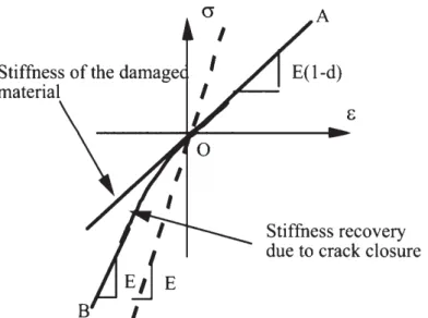
Crack closure effects are of importance when the material is subjected to alternated loads, for instance reinforced concrete structures subjected to earthquakes. The fundamental property of the scalar damage model is that the time derivative of damage is constrained to be positive or zero (second principle of thermodynamics). During load reversals, however, micro cracks are closing progressively and the tangent stiffness of the material should increase while damage is constant (Fig. 1 ).

Stiffness of the damage material

\

A E(l-d)

Stiffness recovery due to crack closure

Material damaged in tension (path OA) and unloaded up to point B

Figure 1. Schematic response of a material subjected to uniaxial compression after being damaged in

tension.

Within isotropic damage modelling, one solution is to introduce two damage scalars (d1,dc),

type of loading. La Borderie ( 1991) developed the corresponding constitutive relations and applied it to concrete. The elastic energy is:

1[ 1 + + 1 -

-plf=- <a> .. <a> ..

+

<a> .. <a> ..

2 £₀(1- d₁) lJ lJ E₀ (1- de) lJ lJ

+

2:JL

(a a

-a?: )]

+

p, d,

f(a) +

p?d,

a

E iJ iJ kk E (1 - d ) E ( 1 - d ) kk

0 0 t 0 c

(9)

where

(a)+

is the positive part of the stress, i.e. the stress tensor expressed in its principal directions with the positive principal stresses only, and

(a)-

=a-

(a-)+.

Inelastic strains due to the growth of damage are also taken into account in this model with a function /(a) introduced in order to represent the progressive vanishing of inelastic strains due to damage in tension when the material is subjected to compression:

/(a) = akk when akk E ]0, oo

lf

(a)

f(a) =(1

+~)a"kk

when akk E]-ac,O]

2ac

/(a)

=

_!!.t:..

akk when akk E [ -oo, -ac]

2

(10)

where ac is the crack closure stress (material parameter). The stress-strain relation reads:

( 11)

Since the model has two damage variables, the evolutionary equations include two yield functions. These functions are constructed on the same principles as the function used for the one scalar model, except that there are two energy release rates associated to the two damage variables respectively:

(12)

The two loading functions are:

(13)

Note that this constitutive relation cannot be integrated explicitly. The stress decomposition into positive and negative parts is not known a priori. Therefore, the conditions of evolution of damage are not known for each integration step. Same as in classical plasticity, the integration of the constitutive relations is performed with an iterative scheme: the equations of the system are the state laws and the evolution laws recast as follows in order to obtain a well-conditioned algebraic system:

1 ( + 1

-£··= <U>··+ <U>··

lJ Eo ( 1 - d₁) lJ Eo ( 1 - de) lJ

+.!JL[U·· _ (} b··] + f1d1 _{IJ(u) + f32de 8, ..}

E₀ lJ kk lJ (1- d 1) ou~i (1-de) lJ ~-Z₁ =

o

Ye- Ze = 0 (14) 1 (1-dt) = I<;<Y,, zl) 1 = R (Y Z ) (1- de) c e' c

Here, F;,

F;;

are calculated from the integrated equation of evolution of damage instead of an incremental one. It does not change the general picture of the integration process, however. The system is written in a matrix form:

1

I-d _t (15)

where matrix

[J]

can be computed and programmed using formal calculus. A full Newton algorithm is implemented in order to solve this non-linear system. Note that there are two sorts of non-linearities: the first one is due to the evolution of damage (i.e. whether damage grows or not), the second is due to crack closure effects. For constant values of the damage variables, the material is orthotropic in the coordinate system of the principal stresses.

3.2.2 Integrated Damage Model

As we saw above, the evolution of damage is very often related to the state of strain. Moreover, it is defined in an explicit, integrated way, which is easier to handle. The damage loading function in Eq. (6) can be redefined as:

where E: is a positive equivalent measure of strain and K is a threshold value. The equation

f

==

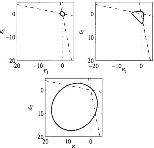
0 represents a loading surface in strain space. For the uniaxial tensile case, the equivalent uniaxial strain in Eq. (16) is straightforward. It is the axial strain. However, for general states of stress, damage evolution should be related to some scalar quantity, function of the state of strain. There are, to this regard, several proposals. For example, an appropriate definition for metals is rooted in the elastic stored energy (Peerlings et al. 1998):

&= -1 &··C··kf&kf

E lJ lJ ( 17)

which is depicted in Figure 2. It is equivalent to the integrated version of the constitutive relation presented in section 2.1. For concrete, Mazars (1984) proposed the following form:

(18)

where &i are the principal strains. A third possibility, which is also mentioned by Peerlings, is

the modified von Mises definition:

"' k-1 1 (k-1)2 2

& - I + - I

- 2k(1-2v) 1 2k (1-2v)2 1 (19)

I1 and 12 are the first invariant of the strain tensor and the second invariant of the deviatoric strain tensor respectively. Only the modified von Mises criterion leads to a new material parameter, namely the factor k. The parameter k is the ratio between uniaxial compressive and uniaxial tensile strengths. These criteria are plotted in figure 2 (with k == 1 0). The loading surfaces (Eqs. 17 -19) are closed contours around the origin. The dashed lines represent the constant uniaxial compression and uniaxial tension stress paths.

The evolution of damage has the same form as in the previous sections:

·

{d

=

h(K) ·

if j(i,K)=O andf(c,K)=Othen _, where d'?:.O

K=& (20) { d == 0 otherwise

i=O

The function h( K) is specific, depending on different models in the literature. For tension only, exponential softening can be used:

where K _{0 ,}

a,

17 are model parameters.

In order to capture the differences of mechanical responses of the material in tension and in compression, Mazars proposed to split the damage variable into two parts and used the equivalent strain defined in Eq. (18):

where dt and de are the damage variables in tension and compression, respectively.

0 ... ~ -10

'

.

-

..A

... :-. ·y-·

~ : \ : \ \ ~ -10 \ \ -20~---~ \ -20~----~----~-~'

-20

0 ... ~ -10 0

-20

-20~---~ -20 -10 0 £1 0 (22)

Figure 2. Contour plots for 8 for the elastic stored energy (top left), Mazars definition (top right), and

the modified von Mises expression (bottom), after Peerlings et al. (1998).

They are combined with the weight coefficients

at

and

ac

defined as functions of the principal values of the strains 8~ and

8ij ,

due to positive and negative stresses (see Mazars,

1984). t 1 t c 1 c 8·· == (1- d) Gk₁

a

8·· == (1-d) Gk₁

a

lJ lJ k/ ' lJ lJ kl (23) =

~[~cf}(c;)+]P

=

2:

3

[{ctXc;)+]P

at

L...J

-2 '

ac

-2 8 8 i=l i=l (24)

In uniaxial tension at= 1 and ae =0. In uniaxial compression ae = 1 and at =0. Hence, dt and

de can be obtained separately from uniaxial tests. The purpose of exponent

f3

is to reduce the effect of damage on the response of the material under shear compared to tension (Pijaudier-Cabot et al. 1991 ). The evolution of damage is provided in an integrated form, as a function of the variable K (Mazars, 1984):

dt = 1- Ko(l-At)-

A,

K exp(B₁ (K- K₀))

Ac

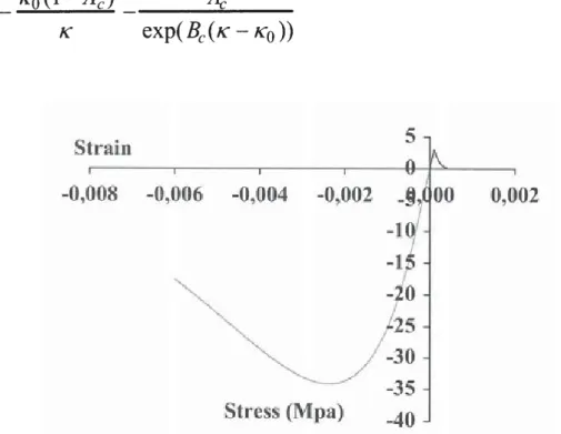
(25) train 5 -0 008 ~0,006 -0 00 - 002 Stress (Mpa) ₄₀

F'i ure 3 Unia ial. r ~ p n.- · f the •nod 1 y . azar 19 4).

Figure 3 shows the uniaxial response of the model in tension and compression with the following parameters: E₀= 30000 MPa, v₀=0.2, _{K 0}=0.0001, A,=l, B, =15000,

Ac

= 1.2,

Be =1500, /3=1.

3.2.3 Damage coupled to plasticity

Elastic damage models or elastic plastic laws are not totally sufficient to correctly capture the constitutive behavior of concrete. In some cases, the calculation of the damage variable is a key point. For instance, it can become essential when coupled effects are considered (coupling between damage and permeability, damage and porosity ... ). Picandet et al. (2001) observed in experiments that there is a relationship between damage and the gas permeability of the material. Damage, measured according to the unloading slope during cyclic compressive loading is related to the variation of permeability, independently from the type of concrete tested (normal concrete, high strength concrete, fiber-reinforced concrete). Thus, the capability of the constitutive model to capture the unloading behavior is essential if a proper evaluation of the permeability is required.

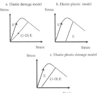
An elastic damage model is not appropriate as irreversible strains cannot be captured: a zero stress corresponds to a zero strain and the value of the damage is thus overestimated (figure 4a). An elastic plastic relation is not adapted (even with softening, see for example Grassl et al, 2002) as the unloading curve always follows the same elastic slope (figure 4b ). An appealing alternative consists in combining these two approaches into an elastic-plastic-damage law. The softening behavior and the decrease in the elastic modulus are so reproduced by the damage part while the plasticity effect accounts for the irreversible strains. With this formulation, experimental unloading can be correctly simulated (figure 4c ).

a. El a tic damage rn . d b. Elastic p~asli" mod t

tre lr .·s

t 11in tra·n

tre ~ s c. ~ la. tic p la li c damage nwdel

train

Figure 4. Unloading response of elastic damage, elastic plastic and elastic plastic damage models.

The plastic model is governed by the following set of equations:

de .. _lj =d&~ _lj +de? _lj

t

eo

e

() ij = ij kl 8 kl

de; = d2.mii

(a',

kJ dkh = d2.h(o-' ,kh)

with the effective stress defined as

(]' .. t lj () .. = -1) (1-d) (26) (27)

where

c,

c

and ~ are respectively the total, elastic and plastic strains, 'A the plastic multiplier and kh the hardening parameter ( 0 ~ kh ~ 1 ). m and h are the flow vectors defined by :

8f m .. ==--lJ

a

t (J'ij 2 8f 8f 3 aa~

.

aa~ h = =

-fis the yield surface and

t;

a function of the stress (Etse and Willam, 1994).

(28)

(29)

with f1 and 1₂ the effective stress invariant and

e

the Lode angle function of the second and

third stress invariant and ranging from [ -n/6 ; n/6]. The evolution of the plastic multiplier is finally given by:

(30)

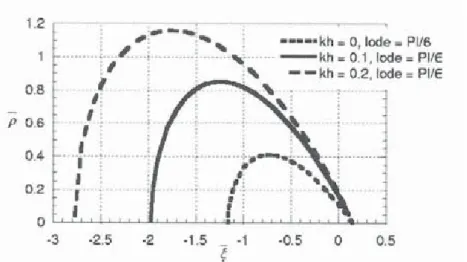
This local problem is solved with an iterative procedure associated to a closest point projection algorithm (see Perez-Foguet et al, 2000). Figure 5 shows the evolution of the yield surface with an increasing hardening parameter kh for simple compression

p ==

K

1

.[:/;,~

== K₂1:, where K1 and K2 are two positive constants).

1 2 k 1 • 0 lode _ P 1/6 k o 1 loo Pile - -kh

=

0.2 lod = Pile 0 o ~~~~~~~~~~~~~~ -3 -2.5 -2 '"1 .5 -0.5 0 0.5

Figure 5. Plastic yield surface. Evolution with the hardening parameter for simple compression (Lode =

As the hardening parameter has a limited value of 1, once it has reached this critical level, hardening is not allowed any more and the yield surface becomes a failure one (constant effective stress).

Figure 6 gives the axial stress - strain curve for a loading in tension. As the development of damage is predominant during simple tension tests, the damage and plastic-damage models are almost equivalent.

0 0.0004 0 .0 6

'xi ,I ra1n

Figure 6. Stress strain curve for simple tension test. Elastic plastic damage formulation.

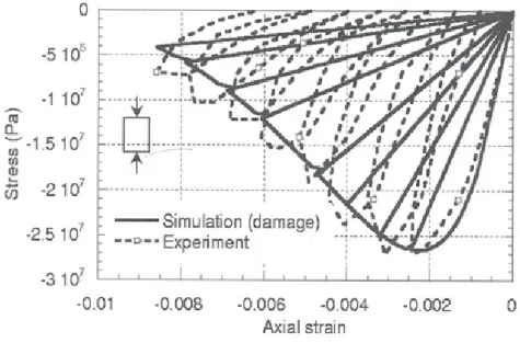
Cyclic compression is a second elementary test. Experimental results are taken from (Sinha et al, 1964). Figure 7 illustrates the numerical response for simple damage law (without any plasticity). With this type of relation, a zero stress corresponds to a zero strain.

-

nJ a.. -; -1 .5 1 o? till Of (ij -2 107 ·2.5 107

···$~--:~·:.:::1"~~~---···:

I I I I ' I : :

'

• • • .. • .. - . - . -- .. - L- - - -- ... •- "'• ••• • • •• ... •.., iftl.-r~,lfl· · "' · - Simulati on (da.m.age) - _, -·EXperiment ~3 1 07 _{!.-....1.--L.-L----t....-....J..._-=-t...,L----L..-J-...L.._....J..._..L.-...JL...L.----J--l_...&...l...l} -0 .01 ~ 0 . 008 -0.006 -0.004 -0.002 0 Axial strai 11

The numerical response of the elastic plastic damage model is given in figure 8. Damage simulates the global softening behaviour of concrete while the plastic part reproduces quantitatively the evolution of the irreversible strains. Experimental and numerical unloading slopes are thus similar, contrary to the simple damage formulation response. If this difference could seem negligible, it is in fact essential if a correct value of the damage needs to be captured. The elastic damage model overestimates d whereas the full plastic damage constitutive law provides more acceptable results.

m

~ -1.5 07 (:ll UlJ

E

-2 1o7 UJ -s2 .. 5 107 -3 1

o

7· 1..-....1.---L..--L..-__,__-'---.J....__JL-....ii.---I..,~~-~-.L...I---~.._._ ... ..._...I-...J -0.01 -0.008 -0.006 -0.004 -0.002 0 Axi1al strain

Figure 8. Cyclic compression test. Elastic plastic damage formulation.

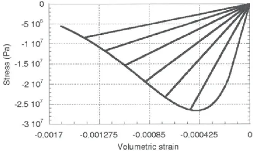
Figure 9 and 10 illustrates the differences between the two approaches tn term of volumetric behaviors. -51

or'

I I I ---- ----·-··. ---· -- ·---2.5 107 -3 10 •s0.0017 1 i -0.0012751 -0.000851 -0.000425 Volumetric strai1 n 0

' ' I o

- ;---- --- --- ---\- --- -:-- -t--·t-

---~--- ----~--- ---!--- --~---2.5 107 : : : : I 1 I I ______ j--- _____

l ___

---~---

_

----L--- ---

i--- __ _

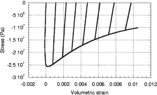
I o ' ' ' ' -3 107 -0.002 0 0.002 0.004 0.006 0.008 0.01 0.012 Volumetric strain

Figure 10. Cyclic compression test. Volumetric behaviour for the plastic damage model.

While, with the simple damage law, the volumetric strains keep negative values, the introduction of plasticity exhibits a change in the volumetric response from contractant (negative volumetric strains) to dilatant, a phenomenon which is experimentally observed (see Sfer et al, 2002 for example).

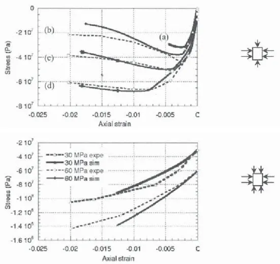
The introduction of plasticity associated with the development of damage plays thus a key role in the numerical simulation of a cyclic compression test. Moreover, the volumetric response, that was totally misevaluated by the elastic damage model, is correctly simulated with the full formulation. In figure 11, numerical results are compared with experiment for different levels of confinement pressures in triaxial experiments (P = 0, 1.5, 4.5, 9, 30 and 60 MPa). Simulations and experiment give similar results. The peak position is quantitatively well reproduced (except for 1.5 MP a ).

The global evolution is also correct: the maximum of the axial stress increases with the pressure and the softening part is less and less significant. When the initial hydrostatic pressure takes higher values, the damage part of the model plays a minor role and plasticity effect becomes predominant.

3.3

Damage Induced Anisotropy

Microcracking is usually geometrically oriented as a result of the loading history on the material. In tension, microcracks are perpendicular to the tensile stress direction, in compression microcracks open parallel to the compressive stress direction. Although a scalar damage model, which does not account for directionality of damage, might be a sufficient approximation in usual applications, i.e. when tensile failure is expected with a quasi-radial loading path, damage induced anisotropy is required for more complex loading histories. The influence of crack closure is needed in the case of alternated loads: microcracks may close and

the effect of damage on the material stiffness disappears. Finally, plastic strains need to be incorporated in the formulation when the material unloads in compression. The following section describes a constitutive relation based on elasto-plastic damage which addresses these issues (Fichant et al. 1999).

0 -2 Hi l!h Ui - 1 -2 0

-

ali 8 I ·1 en · 1.2 (b) ·0.01 ·0.005 IC::: A ial strain ia , · n

Figure 11. Triaxial test with increasing confinement. Axial stress - strain curves for low hydrostatic pressures. Straight lines (black markers) correspond to simulation, dotted lines (white markers) to experiment (on top (a) 0 MPa, (b) 1.5 MPa, (c) 4.5 MPa, (d) 9 MPa).

3.3.1 Principle

The model is based on the approximation of the relationship between the overall stress (latter simply denoted as stress) and the effective stress in the material defined here by the equation:

t CO e t CO ~,..,damaged

)-l

G'·· = ··k1

c

or G'·· = ··kl

c

a

lJ lJ kl lJ lJ klmn mn (31)

h t . h r~

.

e . h 1 . . d

c

damaged . h w ere aiJ Is t e e 1ect1ve stress component, &kf Is t e e astlc strain, an iJkl IS t e

stiffness of the damaged material. We define the relationship between the stress and the effective stress along a finite set of directions of unit vectors

n

at each material point:

3 2

a=

(1-

d(n)

)nial~n

₁, r =

(1-

d(n))

L

(a~n

1 - (nkak,n,) nj) (32)

i=l

a and r are the normal and tangential components of the stress vector respectively. d(n) is a scalar valued quantity which introduces the effect of damage in each direction

ii .

The basis of the model is the numerical interpolation of d (n) (called damage surface) which is approximated by its knowledge over a finite set of directions. The stress is solution of the virtual work equation:

find aij such that V & ~

4

;

aijc~

= J([(I-d(n))n*a;,n1n,

+(1-d(n))(a~nj

-n*a;,n,n,)]

c~nJ

dO

s

(33)

Depending on the interpolation of the damage variable d (n), several forms of damage induced anisotropy can be obtained. Here, it is defined by three scalars in three mutually orthogonal directions. It is the simplest approximation that yields anisotropy of the damaged stiffness of the material. The material is orthotropic with a possibility of rotation of the principal axes of orthotropy.

The stiffness degradation occurs mainly for tensile loads. Hence, the evolution of damage will be indexed on tensile strains. The evolution of damage is controlled by a loading surface

f, which is similar to Eq. (6):

(34)

X _{is an hardening softening variable which is interpolated in the same fashion as the damage}

surface. The initial threshold of damage is &d • The evolution of the damage surface is defined

by an evolution equation inspired from that of an isotropic model: if fl(n·) = 0 and n .• d&~n • > 0

l lj J

. [c)

I+ a(n"c'n ·)) • •

l . .

dd(n)

=

( •

e l ·r~ J exp(-a.(nj 8:nj -&d) ni d&:nj

then n. & .. n . l lj J dz(n·)

=

ni·d&:n₁• else dd(n"')

=

0, dz(n"')

=

0 (35) *

The model parameters are &d and a. Note that the vectors

ii

are the three principal directions

of the incremental strains whenever damage grows. After an incremental growth of damage, the new damage surface is the sum of two ellipsoidal surfaces: the one corresponding to the initial damage surface, and the ellipsoid corresponding to the incremental growth of damage.

the new damage surface is the sum of two ellipsoidal surfaces: the one corresponding to the initial damage surface, and the ellipsoid corresponding to the incremental growth of damage.

3.3.2 Coupling with plasticity

Same as for the isotropic model, we decompose the strain increment in an elastic and plastic one. The evolution of the plastic strain is controlled by a yield function which is expressed in term of the effective stress in the undamaged material. We have implemented in this anisotropic damage model the yield function due to Nadai (1950). It is the combination of two Drucker-Prager functions F} and

F2

with the same hardening evolution:

(36)

where J~ and /~ are the second invariant of the deviatoric effective stress and the first invariant of the effective stress respectively.

w

is the hardening variable and ( Ai, Bi) are four parameters ( i = 1, 2) which were originally related to the ratios of the tensile strength to the compressive strength denoted y and of the biaxial compressive strength to the uniaxial strength denoted

f3 :

c.!..::..l

c

P-1

c

r

c

f3

Al=·•jL.I+y' A2=;22P-I' BI=2;2I+y' fh.=;22P-I (37)

These two ratios are constant in the model:

f3

= 1.16 and

r

= 0.4. The evolution of the plastic strains is associated to these surfaces. The hardening rule is given by:

r

w =qp +w₀ (38)

where q and r are model parameters, w₀ defines the initial reversible domain in the stress space, and p is the effective plastic strain.

3.3.3 Crack closure effects

A decomposition of the stress tensor into a positive and negative part is introduced again: a

=(a)

+

+(a)- ,

where < a> +, and < a

> _

are the positive and negative parts of the stress

tensor. The relationship between the stress and the effective stress defined in Eq. (31) of the model is modified:

(39)

degradation as in tension, de (n) is directly deduced from d(n ). It is defined by the same interpolation as d(n) and along each principal direction i, we have the relation:

( l

a

d.

1-8 ..

d~

= I ( l 'l) , i E [ 1, 3] ₍₃₈₎

a

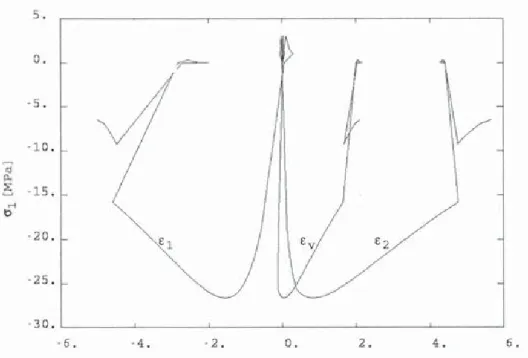
is a model parameter. The constitutive relations contain 6 parameters in addition to the Young's modulus of the material and the Poisson's ratio. Their determination benefits from the fact that in tension, plasticity is negligible. Once the evolution of damage in tension has been fitted, the remaining parameters are fitted from a compression test. Figure 12 shows a typical uniaxial compression-tension response of the model corresponding to a concrete with a tensile strength of 3 MP a and a compressive strength of 40 MP a.

-s ~ L...S · 1! .. · 20 . - 25 , 30 , L---~----~----~---~----~----~ 0 .

Figure 12. Uniaxial tension-compression response of the anisotropic model (longitudinal ( 1 ), transverse (2) and volumetric (v) strains as functions of the compressive stress)

3.4 Non Local Damage

We turn now attention to structural computations with the isotropic damage model. It is well known that when strain softening is encountered (see. Fig. 3 for instance), some difficulties arts e.

Physically, after microcracking has taken place in the first part of the inelastic behavior of concrete, a macroscopic mechanism develops in the form of a damage band. The strains tend

to localize in a specific area of finite dimension (macrocrack) but the model predicts this dimension to be zero, with a vanishing energy dissipation at failure. The stress response of a material point cannot be described locally but has also to consider its neighbourhood in order to take into account microcracks interaction (Askes, 2000). Mathematically (Benallal et a/,

1993, Peerlings et a/, 1996 ), when a material point enters the softening regime, the type of the governing equations changes from elliptic to hyperbolic. The mathematical description becomes ill-posed since the initial and boundary conditions that are meaningful for the elliptic problem are usually not relevant for the hyperbolic part. Numerically, the local formulation of the problem yields a response which is dependant on the smoothness and the orientation of the mesh. Let us consider for example a bar with a variable section under tensile loading whose boundary conditions are given in figure 13. In the damage distribution in figure 14 (a), damage localises only in the most loaded element. If we consider the extreme case of an infinitely fine mesh, this geometrical localisation in a single element yields a fracture without energy dissipation. The local formulation thus exhibits a mesh dependency problem and a regularisation technique has to be added in order to achieve a mesh independent result and damage localisation over several finite elements (Fig. 14b ).

Figure 13. Boundary conditions

Figure 14. Damage distribution (a) local simulation (b) non local simulation. Clear zones correspond to damaged one.

It is now established that non locality, in a gradient or integral format, is mandatory for a proper, consistent, modelling of fracture (see e.g. de Borst et al. 1993). It avoids the difficulties encountered upon material softening and strain localisation. Within a single approach, it encompasses both crack initiation (for which continuum models are very well fitted) and crack propagation (for which discrete fracture approaches have been developed). We shall describe in the following integral and gradient non local damage models.

3.4.1 Integral Model

Consider for instance the scalar damage model in which evolution of damage is controlled by the equivalent strain i:~ introduced by Mazars. The :erinciple of nonlocal continuum models with local strains is to replace the equivalent strain & with its average (Pijaudier-Cabot and

Bazant, 1987): - 1

f -

f

&(x)

=

lf/(s)c(s

+

x)ds with V,.(x)

=

lf/(s)ds Vr(x) n n (39)

where

n

is the volume of the structure, V,.(x) is the representative volume at point x, and

lf/(S) is the weight function, for instance:

(40)

le is the internal length of the non local continuum.

8

replaces the equivalent strain in the evolution of damage. In particular, the loading function becomes f(e,K)

=

&-K. As we will see in section 3.5, it should be noticed that this model is easy to implement in the context of explicit, total strain models. Its extension to plasticity and to implicit incremental relations is awkward. The local tangent stiffness operator relating incremental strains to incremental stresses becomes non symmetric, and more importantly its bandwidth can be very large due to non local interactions. This is one of the reasons why gradient damage models have become popular over the past few years.

3.4.2 Gradient damage model

A simple method to transform the above non local model to a gradient model is to expand the equivalent strain into Taylor series truncated for instance to the second order:

- - oc(x) 0'2 &(x) s2

&(x

+

s)

=

&(x)

+

a

s

+

&2

2!

+ ...

(41) Substitution in Eq. (39) and integration with respect to variable s yields:

- - 2

2-&(x) =2-&(x)+ c V &(x) (42)

where c is a parameter which depends on the type of weight function in Eq. (39). Its dimension is m 2 and it can be regarded as the square of an internal length. Substitution of the new expression of the non local equivalent strain in the non local damage model presented above yields a gradient damage model. Computationally, this model is still delicate to

This difficulty can be solved if an implicit format of the gradient damage model is used. Eq. ( 42) is replaced with

- 2 2-

-c(x)-c V c(x)==c(x) (43)

Here, the definition of the non local equivalent strain is implicit. It is the solution of a Fredholm equation. As shown by Peerlings et al. ( 1996), the implicit form is in fact an exact representation of the integral relation devised by Pijaudier-Cabot and Bazant ( 1987), provided a specific exponential weight function is used.

3.4.3 Extension of the Gradient Approach

In the anisotropic damage models described in section 3.3, the evolution of damage is directional. The evolution of damage is also directional in the microplane-based models and in the smeared crack models. The extension of the gradient damage model to anisotropy, or to any strain-based damage model, can be performed in a very systematic way (Godard, 2001, 2003). The Fredholm equation is written for each strain component Enn :

(44) Therefore, a non local (gradient type) strain tensor is computed within each iteration. It is from this tensor that an equivalent strain can be computed, or that directional damage growth can be devised depending on the type of damage model that is implemented. This extended form of a gradient model has been implemented in the general purpose finite element code "Code Aster" at EDF.

···••

···

··~ ~---~--~~·~·-··--~

...

t

Jl

t

••••••• ...____,.,_ _ _ _ _ :...---'• ...,··--·

----~

160 mm 16 mm • ••••• 480mm 640mm

Figure 15. Bending beam.

~

3.5 Computer implementation of damage models

Since the major effect of damage is a secant stiffness reduction when microcracking progresses, a non-linear computational procedure based on the secant material stiffness seems quite appropriate. This type of algorithm is also widely used when an integral non local damage model is implemented. The major reason is that the tangent stiffness operator (in the case of loading) is far from being straightforward because of non locality.

600

~

"'0 400 "C m 0 _j 2 0 0 0 . . --···---·-~---.-

.

-·--. ____ ... _... . _{~--_...} -0.02 0 o.os, ueT,een~cnil (m ) 1rr 0.08 0.1

Figure 16. Comparison between two non local approaches for different values of the internal length

parameter.

Figure 17. Distribution of damage. Dark zones correspond to damaged one (D = I for black zones,

O<D<l for grey zones and D = 0 for white zones)

The integral relation due to the non local term is discretised according to the finite element mesh used for the analysis and an usual quadrature rule is employed for its evaluation. In finite

are set to zero. The actual volume of integration does not span over the entire volume of 1he solid and the calculation of the integrals requires less computer time and memory as the number of neighbouring integration points is reduced. It should be kept in mind, however, that the secant stiffness algorithm presents serious difficulties, mainly there is no proof of convergence of such an algorithm. In large scale finite element computations, a standard Newton-Raphson algorithm is highly preferable, as convergence is more robust. Such an algorithm relies on the derivation of the consistent tangent stiffness of the material response.

The implementation of the scalar damage model, coupled to the gradient approach is different. The equilibrium equations and the Fredholm equations are solved as a coupled problem. The non local strain tensor can be discretised according to the same finite element grid as the displacements. For a better robustness, a standard Newton-Raphson algorithm is used with a consistent tangent operator that ensures quadratic convergence, if properly implemented.

In order to illustrate results with the integral and gradient damage models, we consider the classical case of a three point bending beam containing a notch. Two different meshes are used (a COARse 890 element and a MEDium 1938 element). Figure 15 shows the beam geometry. Figure 16 presents the comparison between the non local integral and regularised approaches for the medium mesh (se is equal to the square root of c). Choosing the appropriate non local parameters, the two techniques are almost equivalent. Figure 1 7 presents the damage distribution in the half beam for the gradient model. One can see that it is mesh independent.

3.6

Model calibration

The calibration of the model parameters in the non local (integral or gradient) damage model is facing the difficulty of getting at the same time the parameters involved in the evolution of damage K

0 , A1 , B1 , and the internal length le . The first set is a point-wise piece of

information while the influence of the internal length appears in a boundary value problem with non homogeneous strains (by definition,

&

= & ). It follows that it is not possible to calibrate the model parameters in the damage evolution law, without considering the computation of a complete boundary value problem up to failure. Hence the model parameter calibration has to rely on an inverse analysis technique.

The model parameters are optimised so that computational results are as close as possible to the experimental results. The optimisation process used here is based on a Levenberg-Marquardt algorithm, which performs the minimisation of the following functionnal 3(P):

(45)

calibration cannot be performed on a single set of experimental data, e.g. three point bend experiments. One possibility is to perform the calibration from several experiments, and for instance size effect test data.

3.6.1 Size effect tests

Three point bend experiments have been carried out by Le Bellego et al. (2000) on notched geometrically similar specimens of various height D

=

80, 160, and 320 mm, of length L

=

4D, and of thickness b

=

40 mm kept constant. The length-to-height ratio is LID

=

4, the span-to-height ratio is //D

=

3, and the notch length is D/1 0 (Fig. 18). These are mortar specimens with a water-cement ratio of 0.4 and a cement-sand ratio 0.46 (all by weight). The maximal sand grain size is da = 3mm. Experimental and computational data will be also interpreted with the help of Bazant's size effect law, in one of its simplest form (Bazant and Planas, 1998). The nominal strength is obtained with the formula:

3

Fl

a-=---2 b(0.9D)2

where

F

is the peak load. The size effect law reads:

30

0₃

=

320

mm

r---~ 02 = 160 mm

"---~ 0₁ = 80

mm

Figure 18. Geometry of the three point bend size effect tests

(46)

(47)

D0 is a characteristic size, ;;' is the tensile strength of the material, and B is a geometry

-related parameter.

Figure 19 shows the size effect law in a log-log plot. It can be seen that the nominal value of the material strength decreases as the size of the beam increases. This is typical of a damage process in which the process zone is size independent (controlled by the internal length) compared to the structure. For very small sizes, the process zone covers all the specimen and a material strength criterion is expected, while for infinitely large specimens the process zone size is negligible and Linear Elastic Fracture Mechanics should apply.

The calibration of the model parameters from inverse analysis relies first on an accurate finite element representation of each size of specimen. Experience shows that the accuracy of the finite element discretisation in the fracture process zone depends on the ratio of the size of the finite element to the internal length. Therefore, geometrically similar finite element meshes should not be used for the calibration. In order to avoid some possible mesh bias, the finite element size in the process zone should be kept constant and small enough compared to the internal length (at least one third of the internal length). Obviously, the internal length is not known a priori and this requirement is checked at the end of the calibration.

1

a/Btr

1- -

si~e effect law

• , experim,ents

0! 1

~~..-1 ~~~.J...II....J....L.JI...L.L..-...__-l...b...I...I...__

-~LJ,JI

0!1

1

D/[b

10

Figure 19. Experimental results of size effect in three point bend tests.

The optimisation technique has to start from an initial set of model parameters obtained from a manual (trial and error) calibration. This manual process depends on the exact form of the constitutive relation. Therefore, it is difficult to devise a general technique. Still it can be carried out in a rather systematic way as follow: first the model parameters are fitted such that the load deflection curve of one size of specimen is correctly described (usually the medium size). As an initial guess, the internal length lies between 3d a and 5 d a, where d a is the

maximum aggregate size of concrete according to Bazant and Pijaudier-Cabot (1989). The initial damage threshold and the parameters in the equation controlling the damage growth are varied only (in fact, the Young's modulus of the material could be obtained as well from the initial stiffness of the beam). Then, the internal length is adjusted, the other parameters being kept constant, so that the numerical responses for the three specimen sizes are as close as possible to the experimental results. This process requires many calculations, each trial iteration involves three finite element computations. Figure 20 shows such a fit obtained manually.

1200

Fore ~

10

1

00 , (da )

800

600

400

20

1

0

0

0

(c) c- 40mm

- - exper"mental ~numerical

0 05

_' . .

0 1

.

'

0

'

15

Deflexion

(m1

m)

0,2

Figure 20. Manual fit of the damage parameters from size effect tests.

Because there are experimental errors and because the above calibration process is based on a variation of the internal length which is disconnected to the variation of the other model parameters, there are several sets of model parameters which may provide an acceptable fit of the tests data. By acceptable, we mean that the numerical responses are as much as possible within the extreme curves due to experimental dispersion (or within an arbitrary distance from them). The difference between these sets ought to be magnified. For this purpose, the size effect method is quite useful (see Le Bellego et al. 2003).

1 cr/Bft' 0;,1 0~, 011 • upper bound elower bound Alc=7 mm XLc;;;13mm ~Le= 2:0 mm <>Le = 40 mm

1

10

Figure 21. Interpretation of quasi-identical fits on the size effect plot.

Figure 21 shows how several fits obtained manually with different values of the internal length can be distinguished on the size effect plot.

S,E+03 Force (N) 2 E+03 1.E+03 test Lc=0~03 --- Lc=O 04 ... Lc=O ~OS eflexion (m) O.E+OO ---'T---.---~--.---.,..-­

OIE+OO 2,E-05 4 IE-05 6,,E-05 B,E-05

Figure 22. Automatic calibration of the model parameters on the middle size experiment for different -fixed- internal lengths.

For each set of model parameters, the constants in the size effect law have been fitted and the plot on Fig. 21 has been constructed. It is clear on this figure that none of them are consistent with the experimental data. While the quality of the fit is quite hard to decide upon on load -deflexion curves, it is much easier to examine it on the size effect plot.

1200 _{·o ce (da · )} 1000

800

600

400 200 -0 0 0,05 0 1 - I 0,1S 02 Def exion (mm)

Figure 22. Automatic calibration of the model parameters. The dotted lines are the model responses and the plain lines are, for each size, the minimum and maximum curves obtained from the experimental

In order to exemplify the lack of objectivity of the model calibration (i.e. the lack of uniqueness of the result) when a single size of beam is used as the experimental data set, Fig. 22 shows the results of the automatic calibration on the middle size specimen. Three fixed different values of the internal length have been considered. For each one, the optimisation has been performed yielding different values of the damage parameters. The computed responses are the same, in good agreement with the experimental data. Bending of notched beams is quite often used for parameter identification because it is relatively easy to perform compared to tensile tests that are very sensitive to boundary conditions (Carmeliet, 1999). This figure shows that the model cannot be calibrated from inverse analysis of a single load deflexion curve.

Figure 23 shows the result of the optimisation from the three sizes of specimens simultaneously. Compared to the manual fit in Fig. 20, the present set of model parameter provides computational results that are closer to the experiments. We tried to change the initial set of model parameter in order to investigate its stability. Overall, the final sets did not differ very much. The largest difference was found on the internal length, which lied between 40 mm and 50 mm.

3.7 Closure

Continuous damage mechanics is a theory which aims at describing the mechanical effect of cracking and void growth in an elastic material. Isotropic and anisotropic damage models have been presented in this chapter. There is a rather generic technique which permits a rational derivation of damage models, given a level of anisotropy which is defined a priori. In order to be more representative of the concrete mechanical response, damage must be coupled to plasticity. A simple, and classical, technique is to assume that the plastic part of the model is written in term of the effective stress. The same applies to the modelling of rock masses.

Strain-softening, which is typical of concrete and rocks, induces spurious strain localisation. Integral or gradient damage model are solutions to circumvent this problem. A central issue is the calibration of the model parameters, and in particular the experimental determination of the internal length. This can be achieved from size effect test data with the help of inverse analysis of structural responses. It is important, however, to underline that a proper calibration cannot be achieved from the fit of a single experiment. Size effect experiments on geometrically similar specimens, or bending and pure tension tests are required.

Acknowledgements

Financial support from the European Commission through the MAECENAS project (FIS5-2001-00100), through the DIGA RTN network (HPRN-CT-2002-00220), and from the partnership between Electricite de France and the R&DO group through the MECEN project are gratefully acknowledged.

3.8 References

Askes H., 2000, Advanced spatial discretisation strategies for localised failure. mesh adaptivity and meshless methods, PhD Thesis, Delft University of Technology, Faculty of Civil Engineering and Geosciences.

Bazant, Z.P., and Pijaudier-Cabot, G., 1989, Measurement of the characteristic length of non local continuum, J. Engrg. Mech. ASCE, 115, 755-767.

Bazant, Z.P. and Planas, J., 1998, Fracture and size effect in concrete and other quasi brittle Materials, CRC Press.

Benallal A., Billardon R., Geymonat G., 1993, Bifurcation and rate-independent materials, Bifurcation and stability of dissipative systems, CISM Lecture Notes 327, Springer, 1-44. de Borst R., Sluys L.J., Muhlhaus H.B., and Pamin J., 1993, Fundamental issues in finite

element analyses of strain localisation, Engrg. Comput., 10, 99-121.

Carmeliet J., 1999, Optimal estimation of gradient damage parameters from localisation phenomena in quasi-brittle materials, Int.J. Mech. Cohesive Frict. Mats., 4, 1-16.

Etse, G. Willam, K., 1994, Fracture energy formulation for inelastic behavior of plain concrete. J. Engrg. Mech. ASCE, 120, 1983-2011.

Fichant S., La Borderie C., and Pijaudier-Cabot G., 1999, Isotropic and anisotropic descriptions of damage in concrete structures, Int.J. Mech. Cohesive Frict. Mats., 4, pp. 339-359.

Grassl, P. Lundgren, K. Gylltoft, K., 2002, Concrete in compression: a plasticity theory with a novel hardening law, International Journal of Solids and Structures 39:5205-5223.

Godard V., 2001, Modelisation mecanique non locale des materiaux fragiles: delocalisation de la deformation, Stage de DEA de Mecanique, Universite Pierre et Marie Curie.

Godard V., 2003, Modelisation non locale

a

gradients de deformation, Documentation de reference Code_Aster R5.04.02, www.code-aster.org.

La Borderie C., 1991, Phenomenes unilateraux dans un materiau endommageable, These de Doctorat de I 'Universite Paris 6.

Le Bellego C., Dube J-F., Pijaudier-Cabot G., B. Gerard, 2003, Calibration of nonlocal damage model from size effect tests, European Journal of Mechanics A/Solids, 22, 33 --46. Le Bellego, C., Gerard B., and Pijaudier-Cabot G., 2000, Chemomechanical effects in mortar

beams subjected to water hydrolysis, J. Engrg. Mech. ASCE, 126, 266-272. Lemaitre J., 1992, A course on damage mechanics, Springer-Verlag.

Mazars J., 1984, Application de la mecanique de l'endommagement au comportement non lineaire et

a

la rupture du beton de structure, These de Doctorat es Sciences, Universite Paris 6.

Nadai A., 1950, Theory of flow and fracture of solids, Vol. 1, second edition, Me Graw Hill, New York, p. 572.

Peerlings R.H., de Borst R., Brekelmans W.A.M., de Vree J.H.P., 1996, Gradient enhanced damage for quasi-brittle materials, Int. J. Num. Meth. Engrg., 39, 3391-3403.

Peerlings R.H., de Borst R., Brekelmans W.A.M, Geers M.G.D., 1998, Gradient enhanced modelling of concrete fracture, Int.J. Mech. Cohesive Frict. Mats., 3, 323-343.

Picandet, V. Khelidj, A. Bastian, G., 2001, Effect of axial compressive damage on gas permeability of ordinary and high-performance concrete, Cement and Concrete Research, 31, 1525-1532.

Pijaudier-Cabot G. and Bazant Z.P., 1987, Nonlocal damage theory, J. of Engrg. Mech., ASCE, 113, 1512-15 3 3.

Pijaudier-Cabot G., Mazars J., and Pulikowski J., 1991, Steel-concrete bond analysis with nonlocal continuous damage, J. of Structural Engineering, ASCE, 117, 862-882.

Sfer, D., Carol I. Gettu R., Etse, G., 2002, Study of the behavior of concrete under triaxial compression, J. Engrg. Mech. ASCE, 128, 156-163.

Sinha, B.P. Gerstle, K.H. Tulin, L.G., 1964, Stress strain relations for concrete under cyclic loading. Journal of the American concrete institute, 195-211.