HAL Id: hal-01500489
https://hal.sorbonne-universite.fr/hal-01500489
Preprint submitted on 3 Apr 2017
HAL is a multi-disciplinary open access
archive for the deposit and dissemination of
sci-entific research documents, whether they are
pub-lished or not. The documents may come from
teaching and research institutions in France or
abroad, or from public or private research centers.
L’archive ouverte pluridisciplinaire HAL, est
destinée au dépôt et à la diffusion de documents
scientifiques de niveau recherche, publiés ou non,
émanant des établissements d’enseignement et de
recherche français ou étrangers, des laboratoires
publics ou privés.
Efficient Route Tracing from a Single Source
Benoit Donnet, Philippe Raoult, Timur Friedman
To cite this version:
Benoit Donnet, Philippe Raoult, Timur Friedman. Efficient Route Tracing from a Single Source. 2006.
�hal-01500489�
arXiv:cs/0605133v1 [cs.NI] 29 May 2006
Efficient Route Tracing from a Single Source
Benoit Donnet, Philippe Raoult, Timur Friedman
Universit´
e Pierre & Marie Curie, Laboratoire LIP6–CNRS, UMR 7606, Paris, France
Abstract
Traceroute is a networking tool that allows one to dis-cover the path that packets take from a source machine, through the network, to a destination machine. It is widely used as an engineering tool, and also as a scien-tific tool, such as for discovery of the network topology at the IP level. In prior work, authors on this techni-cal report have shown how to improve the efficiency of route tracing from multiple cooperating monitors. How-ever, it is not unusual for a route tracing monitor to operate in isolation. Somewhat different strategies are required for this case, and this report is the first system-atic study of those requirements. Standard traceroute is inefficient when used repeatedly towards multiple desti-nations, as it repeatedly probes the same interfaces close to the source. Others have recognized this inefficiency and have proposed tracing backwards from the desti-nations and stopping probing upon encounter with a previously-seen interface. One of this technical report’s contributions is to quantify for the first time the effi-ciency of this approach. Another contribution is to de-scribe the effect of non-responding destinations on this efficiency. Since a large portion of destination machines do not reply to probe packets, backwards probing from the destination is often infeasible. We propose an al-gorithm to tackle non-responding destinations, and we find that our algorithm can strongly decrease probing redundancy at the cost of a small reduction in node and link discovery.
1
Introduction
Traceroute [1] is a networking diagnostic tool natively available on most of the operating systems. It allows one to determine the path followed by a packet. Traceroute allows therefore to draw up the map of router inter-faces present along the path between a machine S (the source or the monitor ) and a machine D (the destina-tion). Traceroute has also engineering applications as it can be used, for instance, to detect routers that fail in a network. This report proposes and evaluates improve-ments to standard traceroute for tracing routes from a single point.
Today’s most extensive tracing system at the IP inter-face level, skitter [2], uses 24 monitors, each targeting
on the order of one million destinations. In the fash-ion of skitter, scamper [3] makes use of several moni-tors to traceroute IPv6 networks. The Distributed In-ternet MEasurements & Simulations [4] (Dimes) is a measurement infrastructure somewhat similar to the fa-mous SETI@home [5]. SETI@home’s screensaver down-loads and analyzes radio-telescope data. The idea be-hind Dimes is to provide to the research community a publicly downloadable distributed route tracing tool. It was released as a daemon in September 2004. The Dimes agent performs Internet measurements such as traceroute and ping at a low rate, consuming at peak 1KB/sec. At the time of writing this report, Dimes counts more than 8,700 agents scattered over five con-tinents. In the fashion of skitter, scamper [3] makes use of several monitors to traceroute IPv6 networks. Other well known systems, such as Ripe NCC TTM [6] and NlanrAMP [7], each employs a larger set of monitors, on the order of one- to two-hundred, but they avoid probing outside their own network. Scriptroute [8] is a system that allows an ordinary internet user to perform network measurements from several distributed vantage points. It proposes remote measurement execution on PlanetLab nodes [9], through a daemon that implements ping, hop-by-hop bandwidth measurement, and a num-ber of other utilities in addition to traceroute.
Recently, in the context of large-scale internet topol-ogy discovery, we have shown [10] that standard tracer-oute probing (such as skitter) is particularly inefficient due to duplication of effort at two levels: measurements made by an individual monitor that replicate its own work (intra-monitor redundancy), and measurements made by multiple monitors that replicate each other’s work (inter-monitor redundancy). Using skitter data from August 2004, we have quantified both kinds of re-dundancy. We showed that intra-monitor redundancy is high close to each monitor and, with respect to inter-monitor redundancy, we find that most interfaces are visited by all monitors, especially when close to desti-nations. We further proposed an algorithm, Doubletree, for reducing both forms of redundancy at the same time. This technical report focuses more deeply on the intra-monitor redundancy problem. Systems that dis-cover internet topology at IP level from a set of isolated vantage points (i.e., there is no cooperation between monitors) have interest to reduce their intra-monitor
redundancy. By sending much less probes, monitors can probe the network more frequently. The more fre-quent snapshots you have, the more accurate should be your view of the topology. This technical report demon-strates how a monitor can act to reduce its intra-monitor redundancy.
The nature of intra-monitor redundancy suggest to start probing far from the traceroute monitor and probe backwards (i.e., decreasing TTLs), as first noticed by Govindan and Tangmunarunkit [11], Spring et al. [8], Moors [12] and Donnet et al. [10]. However, perform-ing backward probperform-ing from non-cooperative traceroute monitors in the context of intra-monitor redundancy has never been evaluated previously. Even if backward probing is simple to understand, it is not clear how effi-cient it is. This report evaluates the redundancy reduc-tion of backward probing as well as the eventual infor-mation lost compared to standard traceroute.
Nevertheless, backward probing is based on the as-sumption that destinations reply to probes in order to estimate path lengths and the distance of the last hop before the destination. Unfortunately, a large set of des-tinations (40% in our data set) does not reply to probes, probably due to strongly configured firewalls. In this case, backward probing cannot be performed. In this report, we also propose a way to face non-responding destinations. We further propose an efficient algorithm that can handle both cases, i.e., responding and non-responding destinations. We evaluate these algorithms in terms of intra-monitor redundancy and quantity of information lost.
The remainder of this report is organized as follows: Sec. 2 introduces the data set used throughout this tech-nical report; Sec. 3 gives a key for reading quantile plots; Sec. 4 evaluates standard traceroute; Sec. 5 presents and evaluates separately our backward probing algorithms; Sec. 6 compares the different algorithms; finally, Sec. 7 concludes this report by summarizing its principal con-tributions.
2
Data Set
Our study is based on skitter [2] data from August 1st
through 3rd
, 2004. This data set was generated by 24 monitors located in the United States, Canada, the United Kingdom, France, Sweden, the Netherlands, Japan, and New Zealand. The monitors share a com-mon destination set of 971,080 IPv4 addresses. Each monitor cycles through the destination set at its own rate, taking typically three days to complete a cycle. For the purpose of our studies, in order to reduce com-puting time to a manageable level, we worked from a limited destination set of 50,000, randomly chosen from the original set.
Visits to host and router interfaces are the metric
by which we evaluate redundancy. We consider an in-terface to have been visited if its IP address returned by the host or router appears, at least, at one of the hops in a traceroute. Though it would be of inter-est to calculate the load at the host and router level, rather than at the individual interface level, we make no attempt to disambiguate interfaces in order to ob-tain router-level information. The alias resolution tech-niques described by Pansiot and Grad [13], by Govindan and Tangmunarunkit [11], for Mercator, and applied in the iffinder tool from Caida [14], would require active probing beyond the skitter data, preferably at the same time that the skitter data is collected. The methods used by Spring et al. [15], in Rocketfuel, and by Teixeira et al. [16], apply to routers in the network core, and are untested in stub networks. Despite these limitations, we believe that the load on individual interfaces is a useful measure. As Broido and claffy note [17], “interfaces are individual devices, with their own individual processors, memory, buses, and failure modes. It is reasonable to view them as nodes with their own connections.”
How do we account for skitter visits to router and host interfaces? Like many standard traceroute imple-mentations, skitter sends three probe packets for each hop count. An IP address appears thus in a traceroute result if it appears in the replies to, at least, one of the three probes sent (but it may also appear two or three times). For each reply, we account one visit. If none of the three probes are returned, the hop is recorded as non-responding.
Even if an IP address is returned for a given hop count, it might not be valid. Due to the presence of poorly configured routers along traceroute paths, skit-ter occasionally records anomalies such as private IP ad-dresses that are not globally routable. We account for invalid hops as if they were non-responding hops. The addresses that we consider as invalid are a subset of the special-use IPv4 addresses described in RFC 3330 [18]. Specifically, we eliminate visits to the private IP address blocks 10.0.0.0/8, 172.16.0.0/12, and 192.168.0.0/16. We also remove the loopback address block 127.0.0.0/8. In our data set, we find 4,435 different special addresses, more precisely 4,434 are private addresses and only one is a loopback address. Special addresses account for ap-proximately 3% of the entire set of addresses seen in this trace. Though there were no visits in the data to the fol-lowing address blocks, they too would be considered in-valid: the “this network” block 0.0.0.0/8, the 6to4 relay any cast address block 192.88.99.0/24, the benchmark testing block 198.18.0.0/15, the multicast address block 224.0.0.0/4, and the reserved address block formerly known as the Class E addresses, 240.0.0.0/4, which in-cludes the lan broadcast address, 255.255.255.255.
Figure 1: Quantiles key
3
Description of the Plots
In this report, we plot interface redundancy distribu-tions. Since these distributions are generally skewed, quantile plots give us a better sense of the data than would plots of the mean and variance. There are sev-eral possible ways to calculate quantiles. We calculate them in the manner described by Jain [19, p. 194], which is: rounding to the nearest integer value to obtain the index of the element in question, and using the lower integer if the quantile falls exactly halfway between two integers.
Fig. 1 provides a key to reading the quantile plots found in subsequent sections of this report.
A dot marks the median (the 2nd
quartile, or 50th
percentile). The vertical line below the dot delineates the range from the minimum to the 1st
quartile, and leaves a space from the 1st
to the 2nd
quartile. The space above the dot runs from the 2nd
to the 3rd
quartile, and the line above that extends from the 3rd
quartile to the maximum. Small tick bars to either side of the lines mark some additional percentiles: bars to the left for the 10th
and 90th
, and bars to the right for the 5th
and 95th
.
In the case of highly skewed distributions, or distri-butions drawn from small amounts of data, the vertical lines or the spaces between them might not appear. For instance, if there are tick marks but no vertical line above the dot, this means that the 3rd
quartile is iden-tical to the maximum value.
In the figures, each quantile plot sits directly above an accompanying bar chart that indicates the quantity of data upon which the quantiles were based. For each hop count, the bar chart displays the number of interfaces at that distance. For these bar charts, a log scale is used on the vertical axis. This allows us to identify quantiles that are based upon very few interfaces (fewer than twenty, for instance), and so for which the values risk being somewhat arbitrary.
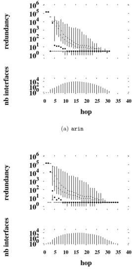
104 102 100 40 35 30 25 20 15 10 5 0 nb interfaces hop 106 105 104 103 102 101 100 redundancy (a) arin 104 102 100 40 35 30 25 20 15 10 5 0 nb interfaces hop 106 105 104 103 102 101 100 redundancy (b) champagne
Figure 2: Redundancy when probing with the pure for-wards algorithm
4
Standard Traceroute
Our basis for comparison is the results from the stan-dard forward tracing algorithm implemented in tracer-oute. All monitors operate from a set of common desti-nations, D. Each monitor probes forward starting from TTL=1 and increasing the TTL hop by hop towards each of the destinations in D in turn. As it probes, a monitor i updates the set, Si, initially empty, of
inter-faces that it has visited.
Evaluating redundancy in the standard traceroute was already published in an authors’ SIGMETRICS 2005 paper [10]. For comparison reasons in the next sections of this report, we summarize in this section our redundancy evaluation of standard traceroute.
Monitor R1 R2 R3 R4 R5 Destination Pr o b in g Se q u e n c e
Figure 3: Pure backwards algorithm
monitors: arin and champagne. The results presented in Fig. 2 are representative of all the skitter monitors. Interested readers might find plots for the 22 other skit-ter monitors in our technical report [20].
Looking first at the histograms for interface counts (the lower half of each plot), we find data consistent with distributions typically seen in such cases. If we were to look at a plot on a linear scale (not shown here), we would see that these distributions display the familiar bell-shaped curve typical of internet interface distance distributions [21]. If we concentrate on champagne, we see that it discovers 92,354 unique and valid IP ad-dresses. The interface distances are distributed with a mean at 17 hops corresponding to a peak of 9,135 interfaces that are visited at that distance.
The quantile plots show the nature of the redundancy problem. Looking at how the redundancy varies by dis-tance, we see that the problem is worse the closer one is to the monitor. This is what we expect given the tree-like structure of routing from a monitor, but here we see how serious the phenomenon is from a quantitative standpoint. For the first two hops from each monitor, the median redundancy is 150,000. A look at the his-tograms shows that there are very few interfaces at these distances. Just one interface for arin, and two (2nd
hop) or three (3rd
hop) for champagne. These close to the monitor interfaces are only visited three times, as rep-resented by the presence of the 5th
and 10th
percentile marks (since there are only two data points, the lower values point is represented by the entire lower quarter of values on the plot).
Beyond three hops, the median redundancy drops rapidly. By the eleventh hop, in both cases, the me-dian is below ten. However, the distributions remain highly skewed. Even fifteen hops out, some interfaces experience a redundancy on the order of several hun-dred visits. With small variations, these patterns are repeated for each of the monitors.
5
Backward Tracing
As seen and discussed in Sec. 4, the most worrisome feature of redundancy in a standard measurement sys-tem is the exceptionally high number of visits to the median interfaces close in to the monitor. Also of con-cern is the heavy tail of the distribution at more distant
hop counts, with a certain number of interfaces consis-tently receiving a high number of visits. Our approach here is to tackle the first problem head-on, and then to see if the second problem remains.
The large number of visits to nodes close in to a mon-itor is easily explained by the tree-like or conal struc-ture of the graph generated by traceroutes from a single monitor, as described by Broido and claffy [17]. There are typically only a few interfaces close to a monitor, and these interfaces must therefore be visited by a large portion of the traceroutes. The solution to this problem is simple, at least in principle: these close in interfaces must be skipped most of the time.
Traceroute works forward from source to destination. Its first set of probes goes just one hop, its second set goes two, and so forth. It would seem that the best way to reduce intra-monitor redundancy is to start fur-ther out and probes backward, i.e., decreasing TTLs. Govindan and Tangmunarunkit [11] do just this in the Mercator system. Using a probing strategy based upon IP address prefixes, Mercator conducts a check before probing the path to a new address that has a prefix P. If paths to an address in P already exist in its database, Mercator starts probing at the highest hop count for a responding router seen on those paths. No results have been published on the performance of this heuristic, though it seems to us an entirely reasonable approach in light of our data.
The Mercator heuristic requires that a guess be made about the relevant prefix length for an address. That guess is based upon the class that the address would have had before the advent of classless inter-domain routing (CIDR) [22]. In this technical report, we have tested a number of simple heuristics that do not require us to hazard such a guess.
Our algorithms work backwards. As illustrated in Fig. 3, a monitor sends its first probes to the desti-nation, its second to one hop short of the destidesti-nation, and so forth. Now arises the question of when to stop backward probing. Based on the tree-like structure of routes emanating from a single point (i.e., the tracer-oute source), we choose a stopping rule based on the set of interfaces previously encountered. A monitor will stop backward probing when an already visited interface is encountered. The only redundancy such a strategy should produce would be on interfaces that are branch-ing points in paths between a monitor and its destina-tions. A backward probing scheme uses the set, Si, of
interfaces that a monitor i has visited. In early prob-ing, Si will have few elements, and so paths should be
traced from the destination almost all the way back to the monitor. Later probing should terminate further and further out, as more and more interfaces are added to Si.
back-wards probing. They arise because of inherent flaws with methods for establishing the number of hops from a monitor to a destination. These methods rely upon the sending of a ping packet (or a scout packet, following Moors’ terminology [12]), and the examination of the time to live (TTL) value in the IP packet that the desti-nation returns. Various heuristics have been described, by Templeton and Levitt [23], Jin et al. [24], Moors [12] and Beverly [25], to guess the original TTL (typically one of a few standard values) based upon the observed value, and thus to guess the hop count from destination to monitor. While these heuristics have been shown to work well, the most serious problem is that they cannot work when the destination does not reply, as is often the case (40.3% in our data). In such a case, a system that takes a backwards probing approach will ideally start from the most distant interface that responds with an ICMP “TTL expired” packet when discarding a hop-limited probe. In practice, this might take some search to locate, adding redundancy.
Furthermore, as established by Paxson [26] based upon data from 1995, and confirmed with data from 2002 by Amini et al. [27], a considerable number of paths in the Internet are asymmetric: most recently almost 70%. This is a less serious problem, however, as the differences in routing often do not translate into considerable differences in hop count. Paxson’s work in-dicated that differences in one or two hops were typical. For the purposes of our simulations we assume that, if a destination does reply to a ping, the system thereby learns the correct number of hops on the forward path.
5.1
Pure Backwards
We simulate an algorithm for backwards probing in which the most distant responding interface is assumed to be known a priori. Called pure backward probing, this algorithm is unrealistic because of its assumption. How-ever, its performance sets a benchmark.Against that al-gorithm, we later compare algorithms that use only in-formation that is actually available to a monitor.
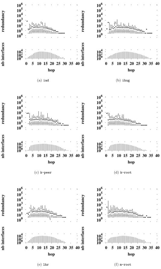
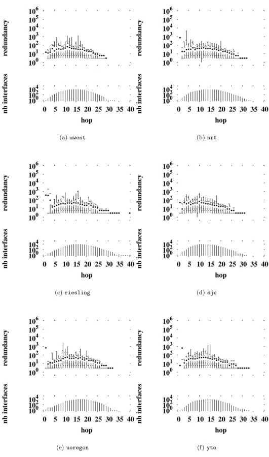
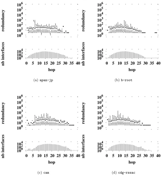
Fig. 4 shows redundancy for monitors running the pure backwards algorithm1
. We notice a significant drop in comparison to the redundancy in straightforward tracerouting shown in Fig. 2. The median drops for the close interfaces, and the distribution tails are signif-icantly shortened overall. However, Figs. 4(a) and 4(b) show still high redundancy for interfaces located one hop from the traceroute source.
We hypothesize that these remanent high redundan-cies close to the monitors are caused by the existence of firewalls or gateways that either do not permit probes to pass through them, or do not permit replies to return.
1Plots for others monitors can be found in an appendix at the
end of this report.
104 102 100 40 35 30 25 20 15 10 5 0 nb interfaces hop 106 105 104 103 102 101 100 redundancy (a) arin 104 102 100 40 35 30 25 20 15 10 5 0 nb interfaces hop 106 105 104 103 102 101 100 redundancy (b) champagne
Figure 4: Redundancy when probing with the pure backwards algorithm
If the destination addresses are invalid, these interfaces could also be default free routers. Under pure back-wards probing, a node situated immediately in front of such a device, whatever it might be, will be visited again and again, for each destination that lies beyond, thus resulting in a high visit count for one of its interfaces. Without any further knowledge, the actual cause of such high redundancy under backwards probing remains for us an open question.
However, Figs. 4(a) and 4(b) show that maximum redundancies are in the thousands, rather that the hun-dreds of thousands as before. Furthermore, median val-ues are a little higher than with standard traceroute. The strong drop in redundancy close to the monitor thus comes at the expense of some increased redundancy further out. The overall effect is one of smoothing the
load.
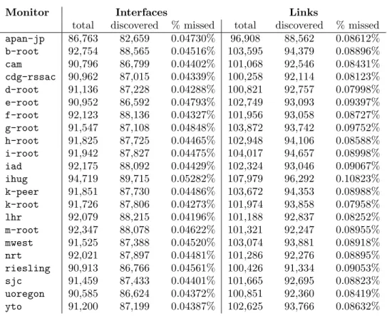
There are costs associated with this drop in redun-dancy. We measure these in terms of the number of interfaces missed, using the set Si of interfaces visited
by the standard algorithm as the reference. For the pure backwards algorithm, the numbers missed are relatively small, as shown in Table 7. Table 7 gives also the cost in term of links missed by the pure backwards algorithm.
Interfaces will necessarily be missed in backwards probing when a hard and fast rule is applied that re-quires probing to stop once an already visited interface is encountered. Any routing change that might have taken place between the monitor and that interface will go unnoticed. A routing system that adopts a back-wards probing algorithm should also adopt a strategy for periodically reprobing certain paths, so as not to miss such changes entirely. So long as the portion of interfaces missed is small, we believe that the develop-ment of such a reprobing strategy can be left to future work.
5.2
Ordinary Backwards
The ordinary backwards algorithm works in much the same way as perfect backwards, but it is a more realistic algorithm. Just as with pure backwards, when a desti-nation responds, the monitor starts probing backwards from the destination until an already visited interface is met. However, when a destination doesn’t reply, the monitor, since it cannot know a priori the most distant responding interface along the path, gives up probing for this particular destination altogether. This is the first of two building blocks that will be used by the al-gorithm presented in Sec. 5.4, and is not intended to be used in isolation.
Approximately 40% the traceroutes in our data set terminate in a non-responding destination. What does this mean in terms of interfaces that are missed? Table 2 shows the costs of not probing these paths combined with the early stopping that is in any case associated with backwards probing. What is remarkable to note is that, compared to perfect backwards probing, ordi-nary backwards probing only misses an additional 16% of interfaces.
Fig. 5 shows trends very similar to those observed with perfect backwards probing, but some high values are no longer present.
5.3
Searching
If we are to use ordinary backwards probing as one element of a larger probing strategy, we need a second el-ement to handle destinations that do not respond. Since the last responding interface on a path to such a destina-tion cannot be known a priori, the monitor must search
104 102 100 40 35 30 25 20 15 10 5 0 nb interfaces hop 106 105 104 103 102 101 100 redundancy (a) arin 104 102 100 40 35 30 25 20 15 10 5 0 nb interfaces hop 106 105 104 103 102 101 100 redundancy (b) champagne
Figure 5: Redundancy when probing with the ordinary backwards algorithm
for it. The search cost is what will make the difference with respect to the pure backwards algorithm.
Our algorithm, labeled searching, now sends its ini-tial probe with a TTL value h. If it receives a response, it continues to probe forwards, to TTLs h + 1, h + 2, and so forth. When the farthest responding interface is found, probing resumes from TTL h − 1, and probes backwards, to TTLs h − 2, h − 3, and so back. If, at any point, a monitor i visits an interface that is in its set Si of interfaces already viewed, probing for that
desti-nation stops. The working of the searching algorithm is illustrated in Fig. 6, where h = 3 and R5 being the last
responding interface.
If the algorithm is supposed to start probing from a midpoint h in the network, we have to decide which value give to h. Doubletree [10], proposed by the
au-Monitor Interfaces Links
total discovered % missed total discovered % missed arin 92,381 88,204 4.52% 101,850 92,602 9.09% champagne 92,354 88,012 4.70% 101,652 92,331 9.17%
Table 1: Interfaces missed by the pure backwards algorithm
Monitor Interfaces Links
total discovered % missed total discovered % missed arin 92,381 73,529 20.40% 101,850 75,163 27.21% champagne 92,354 73,410 20.51% 101,652 74,987 27.24%
Table 2: Interfaces missed by the ordinary backwards algorithm
Monitor R1 R2 R3 R4 R5 Destination Pr o b in g Se q u e n c e
Figure 6: Searching algorithm with h = 3
0 5 10 15 20 25 30 35 40 distance 0.00 0.02 0.04 0.06 0.08 0.10 0.12 proportion arin champagne
Figure 7: Incomplete paths distribution
thors of this report, is a cooperative and efficient al-gorithm for large-scale topology discovery. Each Dou-bletree monitor starts probing at some hop h from it-self, performing forwards probing from h and backwards probing from h − 1. The value h is fixed by each moni-tor according to its probability p of hitting a destination with the very first probe sent. This choice is driven by the risk of probing looking like a distributed denial-of-service (DDoS) attack. Indeed, when probes sent by multiples monitors converge towards a given destina-tion, the probe traffic might appear, for an end-host, as a DDoS attack. Doubletree aims to minimize this risk and, therefore, each monitor chooses an appropriate h value.
In this report, we are not interested in large-scale dis-tributed probing, i.e., from a large set of monitors that cooperate when probing towards a large set of destina-tions. We consider that each monitor works in isolation of others. It does not make sense to choose the h value like Doubletree does.
Fig. 7 shows the incomplete paths distribution, i.e., the distance distribution of the last responding hop when a traceroute does not terminate by hitting the destination. Such a case occurs in approximately 40% of the traceroutes in our dataset. We propose that each monitor tunes its h value with the mean hop count for its incomplete traceroutes. A monitor can easily evalu-ates its own h value by performing a small number of standard traceroutes.
In the special case where there is no response at dis-tance h, the disdis-tance is halved, and halved again until there is a reply, and probing continues forwards and backwards from that point.
Our results in Fig. 8 indicate that low redundancy can be achieved. We tested the heuristic algorithm using only those traceroutes for which the destination does not respond.
However, we notice that close to the monitor, in the fashion of the pure backwards algorithm (see Fig. 4), the redundancy is still high. We believe that this is caused by very short paths for which the last responding inter-face is close to the monitor. For those paths, there is a high probability that sending the first probe at h hops to the monitor will corresponds a non-response. The hvalue will be divided by two, again and again, until reaching a responding interface that will be located close to the monitor, increasing therefore the redundancy of such interfaces.
5.4
Searching Ordinary Backwards
In this section, we study a comprehensive strategy for reducing probing redundancy. We employ ordinary backwards probing, along with the heuristic algorithm
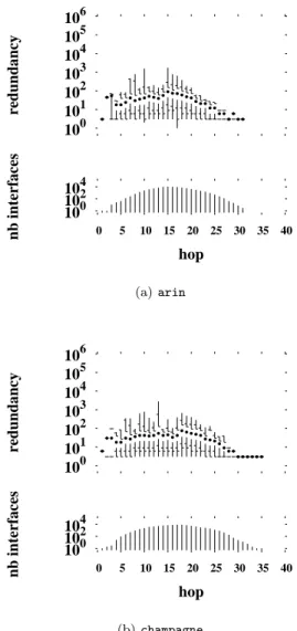
104 102 100 40 35 30 25 20 15 10 5 0 nb interfaces hop 106 105 104 103 102 101 100 redundancy (a) arin 104 102 100 40 35 30 25 20 15 10 5 0 nb interfaces hop 106 105 104 103 102 101 100 redundancy (b) champagne
Figure 8: Redundancy when probing with the searching algorithm
for cases in which the destination does not respond. This algorithm is called searching ordinary backwards.
Fig. 9 shows redundancy reduction similar to that obtained with the other algorithms examined so far.
Table 3 shows the interfaces and links missed when probing with the searching ordinary backwards algo-rithm. Table 3 indicates that the numbers of missed interfaces are a bit smaller (this is specially true for arin) than with the supposedly pure backwards algo-rithm, a surprising fact which will be explained in the next section.
6
Algorithms Comparison
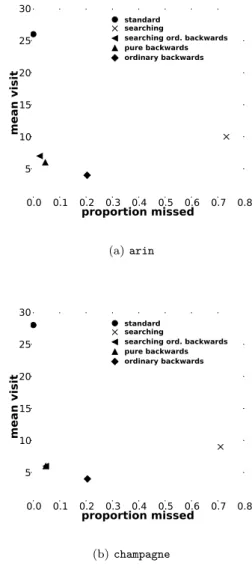
Fig. 10 shows the trade-offs between redundancy and missed address interfaces. Redundancy is here
repre-104 102 100 40 35 30 25 20 15 10 5 0 nb interfaces hop 106 105 104 103 102 101 100 redundancy (a) arin 104 102 100 40 35 30 25 20 15 10 5 0 nb interfaces hop 106 105 104 103 102 101 100 redundancy (b) champagne
Figure 9: Redundancy when probing with the searching ordinary backwards algorithm
sented by the mean number of visits per valid discov-ered interface, and the missed addresses are expressed as a proportion, using the standard traceroute as the reference. Results shown in Fig. 10 are representative for all monitors, as demonstrated by Table 4 giving the mean over the 24 monitors.
Our goal is to avoid both redundancy and missed in-terfaces as much as possible, however there is a trade-off between the two. Extremes are represented by the standard traceroute, which by definition misses no in-terfaces, but has high average redundancy, and by the heuristic algorithm which, having been applied to just those traceroutes for which the destination did not re-spond, necessarily misses a large number of interfaces.
We see that the ordinary backwards provides the low-est redundancy but, as it is applied on only
respond-Monitor Interfaces Links
total discovered % missed total discovered % missed arin 92,381 90,156 2.40% 101,850 94,149 7.57% champagne 92,354 87,946 4.77% 101,652 91,123 10.36%
Table 3: Interfaces missed by the searching ordinary backwards algorithm Algorithms Mean visit Prop. missed
standard 25.08 0
heuristic 9.16 0.74
search. ord. bwd 6.21 0.03
pure bwd 5.58 0.04
ordinary bwd 4 0.2
Table 4: Algorithms comparison - mean
ing traceroutes, it misses a lot of interfaces. The most interesting comparison is between the pure backwards algorithm and searching ordinary backwards. Both are based upon the full set of traceroutes, and so are strictly comparable. The searching ordinary backwards algo-rithm manages to outperform the pure backwards al-gorithm by paying a slight price in terms of increased redundancy (in the case of arin).
7
Conclusion
This technical report addresses the area of efficient probing in the context of traceroute monitors working in isolation from each others. Prior work stated that stan-dard traceroutes are particularly inefficient by repeat-edly reprobing the same interfaces close to the monitor. The solution to this redundancy problem is, at least in principle, simple: those interfaces close to the monitor must be skipped most of the time. It seems that the best way to achieve this solution is to probe backwards from the destinations and stop when encountering a pre-viously seen interface.
In this report, we perform the first careful study of the efficiency of backwards probing, by evaluating it in terms of redundancy reduction and information lost.
Nevertheless, we state that a pure backwards probing algorithm is unrealistic as it is based on the assumption that destinations reply to probes. We therefore propose an algorithm that searches for the last responding inter-face. The key idea of this algorithm is to start probing at some hop h from the monitor, probe forwards from h until the last responding interface and, then, probe backwards from h − 1 until reaching an already discov-ered interface.
We finally propose a realistic algorithm that can han-dle both cases, i.e., responding and non-responding
des-0.0 0.1 0.2 0.3 0.4 0.5 0.6 0.7 0.8 proportion missed 5 10 15 20 25 30 mean visit standard searching
searching ord. backwards pure backwards ordinary backwards (a) arin 0.0 0.1 0.2 0.3 0.4 0.5 0.6 0.7 0.8 proportion missed 5 10 15 20 25 30 mean visit standard searching
searching ord. backwards pure backwards ordinary backwards
(b) champagne
Figure 10: Algorithms comparison
tinations. We evaluate this algorithm and state that it is capable of reducing probe traffic by a factor of 10, while only missing 4% of the interfaces discovered by a standard traceroute.
As a future work, we aim to provide to the research community an implementation of the algorithms dis-cussed in this report.
References
[1] V. Jacobsen et al., “traceroute,” UNIX,” man page, 1989, see source code: ftp://ftp.ee.lbl.gov/traceroute.tar.gz. [2] B. Huffaker, D. Plummer, D. Moore, and k. claffy,
“Topology discovery by active probing,” in Proc. Symposium on Applications and the Internet, Jan. 2002.
[3] “IPv6 scamper,” WAND
Net-work Research Group. Web site: http://www.wand.net.nz/ mjl12/ipv6-scamper/. [4] Y. Shavitt and E. Shir, “DIMES: Let the
in-ternet measure itself,” ACM SIGCOMM Com-puter Communication Review, vol. 35, no. 5, 2005, http://www.netdimes.org.
[5] D. P. Anderson, J. Cobb, E. Korpela, M. Lebof-sky, and D. Werthimer, “SETI@home: An exper-iment in public-resource computing,” Communi-cations of the ACM, vol. 45, no. 11, 2002, see http://setiathome.berkeley.edu/.
[6] F. Georgatos, F. Gruber, D. Karrenberg, M. Santcroos, A. Susanj, H. Uijterwaal, and R. Wilhelm, “Providing active measurements as a regular service for ISPs,” in Proc. Passive and Active Measurement (PAM) Workshop, Apr. 2001. [7] A. McGregor, H.-W. Braun, and J. Brown, “The NLANR network analysis infrastructure,” IEEE Communications Magazine, vol. 38, no. 5, 2000. [8] N. Spring, D. Wetherall, and T. Anderson,
“Scrip-troute: A public internet measurement facility,” in Proc. 4th USENIX Symposium on Internet Technologies and Systems, Mar. 2002, see also http://www.cs.washington.edu/research/ networking/scriptroute/.
[9] PlanetLab Consortium, “PlanetLab project,” 2002, see http://www.planet-lab.org.
[10] B. Donnet, P. Raoult, T. Friedman, and M. Crov-ella, “Efficient algorithms for large-scale topology discovery,” in Proc. ACM SIGMETRICS, 2005, see http://trhome.sourceforge.net.
[11] R. Govindan and H. Tangmunarunkit, “Heuristics for internet map discovery,” in Proc. IEEE INFO-COM, Mar. 2000.
[12] T. Moors, “Streamlining traceroute by estimating path lengths,” in Proc. IEEE International Work-shop on IP Operations and Management (IPOM), Oct. 2004.
[13] J. J. Pansiot and D. Grad, “On routes and multi-cast trees in the internet,” ACM SIGCOMM Com-puter Communication Review, vol. 28, no. 1, pp. 41–50, Jan. 1998.
[14] K. Keys, “iffinder,” a tool for mapping interfaces to routers. See http://www.caida.org/tools/measurement/ iffinder/.
[15] N. Spring, R. Mahajan, and D. Wetherall, “Mea-suring ISP topologies with Rocketfuel,” in Proc. ACM SIGCOMM, Aug. 2002.
[16] R. Teixeira, K. Marzullo, S. Savage, and G. Voelker, “In search of path diversity in ISP net-works,” in Proc. ACM SIGCOMM Internet Mea-surement Conference (IMC), Oct. 2003.
[17] A. Broido and k. claffy, “Internet topology: Con-nectivity of IP graphs,” in Proc. SPIE Interna-tional Symposium on Convergence of IT and Com-munication, Aug. 2001.
[18] IANA, “Special-use IPv4 addresses,” Internet En-gineering Task Force, RFC 3330, 2002.
[19] R. K. Jain, The Art of Computer Systems Perfor-mance Analysis. John Wiley, 1991.
[20] B. Donnet, P. Raoult, T. Friedman, and M. Crov-ella, “Efficient algorithms for large-scale topology discovery,” arXiv, cs.NI 0411013 v1, Nov. 2004. [21] F. Begtasevic and P. Van Mieghem, “Measurement
of the hopcount in the internet,” in Proc. Passive and Active Measurement Workshop (PAM), Apr. 2001.
[22] V. Fuller, T. Li, J. Yu, and K. Varadhan, “Class-less inter-domain routing (CIDR): an address as-signment and aggregation strategy,” Internet En-gineering Task Force, RFC 1519, Sep. 1993. [23] S. J. Templeton and K. E. Levitt, “Detecting
spoofed packets,” in Proc. Third DARPA Informa-tion Survivability Conference and ExposiInforma-tion (DIS-CEX III), Apr. 2003.
[24] C. Jin, H. Wang, and K. G. Shin, “Hop-count fil-tering: An effective defense against spoofed DDoS traffic,” in Proc. ACM Conference on Computer and Communication Security (CCS), Oct. 2003. [25] R. Beverly, “A robust classifier for passive TCP/IP
fingerprinting,” in Proc. Passive and Active Mea-surement Workshop (PAM), Apr. 2004.
[26] V. Paxson, “End-to-end routing behavior in the in-ternet,” in Proc. ACM SIGCOMM, Aug. 1996.
[27] L. D. Amini, A. Shaikh, and H. G. Schulzrinne, “Is-sues with inferring internet topological attributes,” in Proc. SPIE Internet Performance and Control of Network Systems, Aug. 2002.
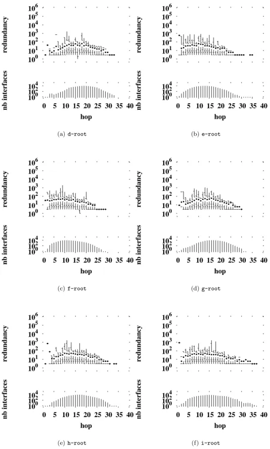
A
Pure Backwards
A.1
Redundancy Reduction
104 102 100 40 35 30 25 20 15 10 5 0 nb interfaces hop 106 105 104 103 102 101 100 redundancy (a) apan-jp 104 102 100 40 35 30 25 20 15 10 5 0 nb interfaces hop 106 105 104 103 102 101 100 redundancy (b) b-root 104 102 100 40 35 30 25 20 15 10 5 0 nb interfaces hop 106 105 104 103 102 101 100 redundancy (c) cam 104 102 100 40 35 30 25 20 15 10 5 0 nb interfaces hop 106 105 104 103 102 101 100 redundancy (d) cdg-rssac
104 102 100 40 35 30 25 20 15 10 5 0 nb interfaces hop 106 105 104 103 102 101 100 redundancy (a) d-root 104 102 100 40 35 30 25 20 15 10 5 0 nb interfaces hop 106 105 104 103 102 101 100 redundancy (b) e-root 104 102 100 40 35 30 25 20 15 10 5 0 nb interfaces hop 106 105 104 103 102 101 100 redundancy (c) f-root 104 102 100 40 35 30 25 20 15 10 5 0 nb interfaces hop 106 105 104 103 102 101 100 redundancy (d) g-root 104 102 100 40 35 30 25 20 15 10 5 0 nb interfaces hop 106 105 104 103 102 101 100 redundancy (e) h-root 104 102 100 40 35 30 25 20 15 10 5 0 nb interfaces hop 106 105 104 103 102 101 100 redundancy (f) i-root
104 102 100 40 35 30 25 20 15 10 5 0 nb interfaces hop 106 105 104 103 102 101 100 redundancy (a) iad 104 102 100 40 35 30 25 20 15 10 5 0 nb interfaces hop 106 105 104 103 102 101 100 redundancy (b) ihug 104 102 100 40 35 30 25 20 15 10 5 0 nb interfaces hop 106 105 104 103 102 101 100 redundancy (c) k-peer 104 102 100 40 35 30 25 20 15 10 5 0 nb interfaces hop 106 105 104 103 102 101 100 redundancy (d) k-root 104 102 100 40 35 30 25 20 15 10 5 0 nb interfaces hop 106 105 104 103 102 101 100 redundancy (e) lhr 104 102 100 40 35 30 25 20 15 10 5 0 nb interfaces hop 106 105 104 103 102 101 100 redundancy (f) m-root
104 102 100 40 35 30 25 20 15 10 5 0 nb interfaces hop 106 105 104 103 102 101 100 redundancy (a) mwest 104 102 100 40 35 30 25 20 15 10 5 0 nb interfaces hop 106 105 104 103 102 101 100 redundancy (b) nrt 104 102 100 40 35 30 25 20 15 10 5 0 nb interfaces hop 106 105 104 103 102 101 100 redundancy (c) riesling 104 102 100 40 35 30 25 20 15 10 5 0 nb interfaces hop 106 105 104 103 102 101 100 redundancy (d) sjc 104 102 100 40 35 30 25 20 15 10 5 0 nb interfaces hop 106 105 104 103 102 101 100 redundancy (e) uoregon 104 102 100 40 35 30 25 20 15 10 5 0 nb interfaces hop 106 105 104 103 102 101 100 redundancy (f) yto
A.2
Losses
Monitor Interfaces Links
total discovered % missed total discovered % missed apan-jp 86,763 82,659 0.04730% 96,908 88,562 0.08612% b-root 92,754 88,565 0.04516% 103,595 94,379 0.08896% cam 90,796 86,799 0.04402% 101,068 92,546 0.08431% cdg-rssac 90,962 87,015 0.04339% 100,258 92,114 0.08123% d-root 91,136 87,228 0.04288% 100,821 92,757 0.07998% e-root 90,952 86,592 0.04793% 102,749 93,093 0.09397% f-root 92,123 88,136 0.04327% 101,956 93,058 0.08727% g-root 91,547 87,108 0.04848% 103,872 93,742 0.09752% h-root 91,825 87,725 0.04465% 102,948 94,106 0.08588% i-root 91,942 87,827 0.04475% 104,017 94,657 0.08998% iad 92,175 88,092 0.04429% 102,324 93,046 0.09067% ihug 94,719 89,715 0.05282% 107,979 96,292 0.10823% k-peer 91,851 87,730 0.04486% 103,672 94,353 0.08988% k-root 91,726 87,806 0.04273% 101,974 93,858 0.07958% lhr 92,079 88,215 0.04196% 101,188 92,837 0.08252% m-root 92,347 88,078 0.04622% 101,321 92,247 0.08955% mwest 91,525 87,388 0.04520% 103,074 93,881 0.08918% nrt 92,021 87,897 0.04481% 101,286 92,276 0.08895% riesling 90,913 86,766 0.04561% 100,426 91,334 0.09053% sjc 91,459 87,433 0.04401% 101,665 92,695 0.08823% uoregon 90,585 86,624 0.04372% 100,851 92,360 0.08419% yto 91,200 87,199 0.04387% 102,625 93,766 0.08632%
B
Ordinary Backwards
B.1
Redundancy Reduction
104 102 100 40 35 30 25 20 15 10 5 0 nb interfaces hop 106 105 104 103 102 101 100 redundancy (a) apan-jp 104 102 100 40 35 30 25 20 15 10 5 0 nb interfaces hop 106 105 104 103 102 101 100 redundancy (b) b-root 104 102 100 40 35 30 25 20 15 10 5 0 nb interfaces hop 106 105 104 103 102 101 100 redundancy (c) cam 104 102 100 40 35 30 25 20 15 10 5 0 nb interfaces hop 106 105 104 103 102 101 100 redundancy (d) cdg-rssac104 102 100 40 35 30 25 20 15 10 5 0 nb interfaces hop 106 105 104 103 102 101 100 redundancy (a) d-root 104 102 100 40 35 30 25 20 15 10 5 0 nb interfaces hop 106 105 104 103 102 101 100 redundancy (b) e-root 104 102 100 40 35 30 25 20 15 10 5 0 nb interfaces hop 106 105 104 103 102 101 100 redundancy (c) f-root 104 102 100 40 35 30 25 20 15 10 5 0 nb interfaces hop 106 105 104 103 102 101 100 redundancy (d) g-root 104 102 100 40 35 30 25 20 15 10 5 0 nb interfaces hop 106 105 104 103 102 101 100 redundancy (e) h-root 104 102 100 40 35 30 25 20 15 10 5 0 nb interfaces hop 106 105 104 103 102 101 100 redundancy (f) i-root
104 102 100 40 35 30 25 20 15 10 5 0 nb interfaces hop 106 105 104 103 102 101 100 redundancy (a) iad 104 102 100 40 35 30 25 20 15 10 5 0 nb interfaces hop 106 105 104 103 102 101 100 redundancy (b) ihug 104 102 100 40 35 30 25 20 15 10 5 0 nb interfaces hop 106 105 104 103 102 101 100 redundancy (c) k-peer 104 102 100 40 35 30 25 20 15 10 5 0 nb interfaces hop 106 105 104 103 102 101 100 redundancy (d) k-root 104 102 100 40 35 30 25 20 15 10 5 0 nb interfaces hop 106 105 104 103 102 101 100 redundancy (e) lhr 104 102 100 40 35 30 25 20 15 10 5 0 nb interfaces hop 106 105 104 103 102 101 100 redundancy (f) m-root
104 102 100 40 35 30 25 20 15 10 5 0 nb interfaces hop 106 105 104 103 102 101 100 redundancy (a) mwest 104 102 100 40 35 30 25 20 15 10 5 0 nb interfaces hop 106 105 104 103 102 101 100 redundancy (b) nrt 104 102 100 40 35 30 25 20 15 10 5 0 nb interfaces hop 106 105 104 103 102 101 100 redundancy (c) riesling 104 102 100 40 35 30 25 20 15 10 5 0 nb interfaces hop 106 105 104 103 102 101 100 redundancy (d) sjc 104 102 100 40 35 30 25 20 15 10 5 0 nb interfaces hop 106 105 104 103 102 101 100 redundancy (e) uoregon 104 102 100 40 35 30 25 20 15 10 5 0 nb interfaces hop 106 105 104 103 102 101 100 redundancy (f) yto
B.2
Losses
Monitor Interfaces Links
total discovered % missed total discovered % missed apan-jp 86,763 68,105 0.21504% 96,908 70796 0,26945% b-root 92,754 73,673 0.20571% 103,595 76701 0,25960% cam 90,796 72,239 0.20438% 101,068 75367 0,25429% cdg-rssac 90,962 72,345 0.20466% 100,258 74897 0,25295% d-root 91,136 72,708 0.20220% 100,821 75669 0,24947% e-root 90,952 71,967 0.20873% 102,749 75477 0,26542% f-root 92,123 73,389 0.20335% 101,956 75454 0,25993% g-root 91,547 72,573 0.20726% 103,872 76349 0,26497% h-root 91,825 73,016 0.20483% 102,948 76598 0,25595% i-root 91,942 73,232 0.20349% 104,017 77063 0,25913% iad 92,175 73,285 0.20493% 102,324 75317 0,26393% ihug 94,719 74,549 0.21294% 107,979 77792 0,27956% k-peer 91,851 72,954 0.20573% 103,672 76607 0,26106% k-root 91,726 73,100 0.20306% 101,974 76451 0,25028% lhr 92,079 73,329 0.20362% 101,188 75229 0,25654% m-root 92,347 73,112 0.20829% 101,321 74611 0,26361% mwest 91,525 72,722 0.20544% 103,074 76388 0,25890% nrt 92,021 73,137 0.20521% 101,286 74612 0,26335% riesling 90,913 72,126 0.20664% 100,426 73859 0,26454% sjc 91,459 72,762 0.20443% 101,665 74936 0,26291% uoregon 90,585 72,082 0.20426% 100,851 75256 0,2537% yto 91,200 72,471 0.20536% 102,625 76155 0,25792%
C
Searching
C.1
Redundancy Reduction
104 102 100 40 35 30 25 20 15 10 5 0 nb interfaces hop 106 105 104 103 102 101 100 redundancy (a) apan-jp 104 102 100 40 35 30 25 20 15 10 5 0 nb interfaces hop 106 105 104 103 102 101 100 redundancy (b) b-root 104 102 100 40 35 30 25 20 15 10 5 0 nb interfaces hop 106 105 104 103 102 101 100 redundancy (c) cam 104 102 100 40 35 30 25 20 15 10 5 0 nb interfaces hop 106 105 104 103 102 101 100 redundancy (d) cdg-rssac104 102 100 40 35 30 25 20 15 10 5 0 nb interfaces hop 106 105 104 103 102 101 100 redundancy (a) d-root 104 102 100 40 35 30 25 20 15 10 5 0 nb interfaces hop 106 105 104 103 102 101 100 redundancy (b) e-root 104 102 100 40 35 30 25 20 15 10 5 0 nb interfaces hop 106 105 104 103 102 101 100 redundancy (c) f-root 104 102 100 40 35 30 25 20 15 10 5 0 nb interfaces hop 106 105 104 103 102 101 100 redundancy (d) g-root 104 102 100 40 35 30 25 20 15 10 5 0 nb interfaces hop 106 105 104 103 102 101 100 redundancy (e) h-root 104 102 100 40 35 30 25 20 15 10 5 0 nb interfaces hop 106 105 104 103 102 101 100 redundancy (f) i-root
104 102 100 40 35 30 25 20 15 10 5 0 nb interfaces hop 106 105 104 103 102 101 100 redundancy (a) iad 104 102 100 40 35 30 25 20 15 10 5 0 nb interfaces hop 106 105 104 103 102 101 100 redundancy (b) ihug 104 102 100 40 35 30 25 20 15 10 5 0 nb interfaces hop 106 105 104 103 102 101 100 redundancy (c) k-peer 104 102 100 40 35 30 25 20 15 10 5 0 nb interfaces hop 106 105 104 103 102 101 100 redundancy (d) k-root 104 102 100 40 35 30 25 20 15 10 5 0 nb interfaces hop 106 105 104 103 102 101 100 redundancy (e) lhr 104 102 100 40 35 30 25 20 15 10 5 0 nb interfaces hop 106 105 104 103 102 101 100 redundancy (f) m-root
104 102 100 40 35 30 25 20 15 10 5 0 nb interfaces hop 106 105 104 103 102 101 100 redundancy (a) mwest 104 102 100 40 35 30 25 20 15 10 5 0 nb interfaces hop 106 105 104 103 102 101 100 redundancy (b) nrt 104 102 100 40 35 30 25 20 15 10 5 0 nb interfaces hop 106 105 104 103 102 101 100 redundancy (c) riesling 104 102 100 40 35 30 25 20 15 10 5 0 nb interfaces hop 106 105 104 103 102 101 100 redundancy (d) sjc 104 102 100 40 35 30 25 20 15 10 5 0 nb interfaces hop 106 105 104 103 102 101 100 redundancy (e) uoregon 104 102 100 40 35 30 25 20 15 10 5 0 nb interfaces hop 106 105 104 103 102 101 100 redundancy (f) yto
C.2
Incomplete Paths
0 5 10 15 20 25 30 35 40 distance 0.00 0.02 0.04 0.06 0.08 0.10 0.12 proportion (a) apan-jp 0 5 10 15 20 25 30 35 40 distance 0.00 0.02 0.04 0.06 0.08 0.10 0.12 proportion (b) b-root 0 5 10 15 20 25 30 35 40 distance 0.00 0.02 0.04 0.06 0.08 0.10 0.12 proportion (c) cam 0 5 10 15 20 25 30 35 40 distance 0.00 0.02 0.04 0.06 0.08 0.10 0.12 proportion (d) cdg-rssac0 5 10 15 20 25 30 35 40 distance 0.00 0.02 0.04 0.06 0.08 0.10 0.12 proportion (a) d-root 0 5 10 15 20 25 30 35 40 distance 0.00 0.02 0.04 0.06 0.08 0.10 0.12 proportion (b) e-root 0 5 10 15 20 25 30 35 40 distance 0.00 0.02 0.04 0.06 0.08 0.10 0.12 proportion (c) f-root 0 5 10 15 20 25 30 35 40 distance 0.00 0.02 0.04 0.06 0.08 0.10 0.12 proportion (d) g-root 0 5 10 15 20 25 30 35 40 distance 0.00 0.02 0.04 0.06 0.08 0.10 0.12 proportion (e) h-root 0 5 10 15 20 25 30 35 40 distance 0.00 0.02 0.04 0.06 0.08 0.10 0.12 proportion (f) i-root
0 5 10 15 20 25 30 35 40 distance 0.00 0.02 0.04 0.06 0.08 0.10 0.12 proportion (a) iad 0 5 10 15 20 25 30 35 40 distance 0.00 0.02 0.04 0.06 0.08 0.10 0.12 proportion (b) ihug 0 5 10 15 20 25 30 35 40 distance 0.00 0.02 0.04 0.06 0.08 0.10 0.12 proportion (c) k-peer 0 5 10 15 20 25 30 35 40 distance 0.00 0.02 0.04 0.06 0.08 0.10 0.12 proportion (d) k-root 0 5 10 15 20 25 30 35 40 distance 0.00 0.02 0.04 0.06 0.08 0.10 0.12 proportion (e) lhr 0 5 10 15 20 25 30 35 40 distance 0.00 0.02 0.04 0.06 0.08 0.10 0.12 proportion (f) m-root
0 5 10 15 20 25 30 35 40 distance 0.00 0.02 0.04 0.06 0.08 0.10 0.12 proportion (a) mwest 0 5 10 15 20 25 30 35 40 distance 0.00 0.02 0.04 0.06 0.08 0.10 0.12 proportion (b) nrt 0 5 10 15 20 25 30 35 40 distance 0.00 0.02 0.04 0.06 0.08 0.10 0.12 proportion (c) riesling 0 5 10 15 20 25 30 35 40 distance 0.00 0.02 0.04 0.06 0.08 0.10 0.12 proportion (d) sjc 0 5 10 15 20 25 30 35 40 distance 0.00 0.02 0.04 0.06 0.08 0.10 0.12 proportion (e) uoregon 0 5 10 15 20 25 30 35 40 distance 0.00 0.02 0.04 0.06 0.08 0.10 0.12 proportion (f) yto
D
Searching Ordinary Backwards
D.1
Redundancy Reduction
104 102 100 40 35 30 25 20 15 10 5 0 nb interfaces hop 106 105 104 103 102 101 100 redundancy (a) apan-jp 104 102 100 40 35 30 25 20 15 10 5 0 nb interfaces hop 106 105 104 103 102 101 100 redundancy (b) b-root 104 102 100 40 35 30 25 20 15 10 5 0 nb interfaces hop 106 105 104 103 102 101 100 redundancy (c) cam 104 102 100 40 35 30 25 20 15 10 5 0 nb interfaces hop 106 105 104 103 102 101 100 redundancy (d) cdg-rssac104 102 100 40 35 30 25 20 15 10 5 0 nb interfaces hop 106 105 104 103 102 101 100 redundancy (a) d-root 104 102 100 40 35 30 25 20 15 10 5 0 nb interfaces hop 106 105 104 103 102 101 100 redundancy (b) e-root 104 102 100 40 35 30 25 20 15 10 5 0 nb interfaces hop 106 105 104 103 102 101 100 redundancy (c) f-root 104 102 100 40 35 30 25 20 15 10 5 0 nb interfaces hop 106 105 104 103 102 101 100 redundancy (d) g-root 104 102 100 40 35 30 25 20 15 10 5 0 nb interfaces hop 106 105 104 103 102 101 100 redundancy (e) h-root 104 102 100 40 35 30 25 20 15 10 5 0 nb interfaces hop 106 105 104 103 102 101 100 redundancy (f) i-root
104 102 100 40 35 30 25 20 15 10 5 0 nb interfaces hop 106 105 104 103 102 101 100 redundancy (a) iad 104 102 100 40 35 30 25 20 15 10 5 0 nb interfaces hop 106 105 104 103 102 101 100 redundancy (b) ihug 104 102 100 40 35 30 25 20 15 10 5 0 nb interfaces hop 106 105 104 103 102 101 100 redundancy (c) k-peer 104 102 100 40 35 30 25 20 15 10 5 0 nb interfaces hop 106 105 104 103 102 101 100 redundancy (d) k-root 104 102 100 40 35 30 25 20 15 10 5 0 nb interfaces hop 106 105 104 103 102 101 100 redundancy (e) lhr 104 102 100 40 35 30 25 20 15 10 5 0 nb interfaces hop 106 105 104 103 102 101 100 redundancy (f) m-root
104 102 100 40 35 30 25 20 15 10 5 0 nb interfaces hop 106 105 104 103 102 101 100 redundancy (a) mwest 104 102 100 40 35 30 25 20 15 10 5 0 nb interfaces hop 106 105 104 103 102 101 100 redundancy (b) nrt 104 102 100 40 35 30 25 20 15 10 5 0 nb interfaces hop 106 105 104 103 102 101 100 redundancy (c) riesling 104 102 100 40 35 30 25 20 15 10 5 0 nb interfaces hop 106 105 104 103 102 101 100 redundancy (d) sjc 104 102 100 40 35 30 25 20 15 10 5 0 nb interfaces hop 106 105 104 103 102 101 100 redundancy (e) uoregon 104 102 100 40 35 30 25 20 15 10 5 0 nb interfaces hop 106 105 104 103 102 101 100 redundancy (f) yto
D.2
Losses
Monitor Interfaces Links
total discovered % missed total discovered % missed apan-jp 86763 83,674 0.03560% 96,908 88,147 0.09040% b-root 92754 89,540 0.03465% 103,595 94,469 0.08809% cam 90796 88,278 0.02773% 101,068 93,822 0.07169% cdg-rssac 90962 87,958 0.03302% 100,258 92,844 0.07394% d-root 91136 89,167 0.02160% 100,821 94,634 0.06136% e-root 90952 88,831 0.02332% 102,749 95,018 0.07524% f-root 92123 90,926 0.01299% 101,956 95,770 0.06067% g-root 91547 89,480 0.02257% 103,872 95,335 0.08218% h-root 91825 88,914 0.03170% 102,948 94,040 0.08652% i-root 91942 88,158 0.04115% 104,017 94,484 0.09164% iad 92175 90,374 0.01953% 102,324 95,031 0.07127% ihug 94719 91,882 0.02995% 107,979 98,129 0.09122% k-peer 91851 89,431 0.02634% 103,672 96,780 0.06647% k-root 91726 89,715 0.02192% 101,974 95,884 0.05972% lhr 92079 89,877 0.02391% 101,188 94,754 0.06358% m-root 92347 89,448 0.03139% 101,321 93,277 0.07939% mwest 91525 89,953 0.01717% 103,074 96,561 0.06318% nrt 92021 89,825 0.02386% 101,286 93,955 0.07237% riesling 90913 87,681 0.03555% 100,426 91,518 0.08870% sjc 91459 89,299 0.02361% 101,665 93,713 0.07821% uoregon 90585 87,990 0.02864% 100,851 92,971 0.07813% yto 91200 89,541 0.01819% 102,625 95,834 0.066173%
E
Algorithms Comparison
0.0 0.1 0.2 0.3 0.4 0.5 0.6 0.7 0.8 proportion missed 5 10 15 20 25 30 mean visit standard searching searching ord. backwards pure backwards ordinary backwards (a) apan-jp 0.0 0.1 0.2 0.3 0.4 0.5 0.6 0.7 0.8 proportion missed 5 10 15 20 25 30 mean visit standard searching searching ord. backwards pure backwards ordinary backwards (b) b-root 0.0 0.1 0.2 0.3 0.4 0.5 0.6 0.7 0.8 proportion missed 5 10 15 20 25 30 mean visit standard searching searching ord. backwards pure backwards ordinary backwards (c) cam 0.0 0.1 0.2 0.3 0.4 0.5 0.6 0.7 0.8 proportion missed 5 10 15 20 25 30 mean visit standard searching searching ord. backwards pure backwards ordinary backwards(d) cdg-rssac
0.0 0.1 0.2 0.3 0.4 0.5 0.6 0.7 0.8 proportion missed 5 10 15 20 25 30 mean visit standard searching searching ord. backwards pure backwards ordinary backwards (a) d-root 0.0 0.1 0.2 0.3 0.4 0.5 0.6 0.7 0.8 proportion missed 5 10 15 20 25 30 mean visit standard searching searching ord. backwards pure backwards ordinary backwards (b) e-root 0.0 0.1 0.2 0.3 0.4 0.5 0.6 0.7 0.8 proportion missed 5 10 15 20 25 30 mean visit standard searching searching ord. backwards pure backwards ordinary backwards (c) f-root 0.0 0.1 0.2 0.3 0.4 0.5 0.6 0.7 0.8 proportion missed 5 10 15 20 25 30 mean visit standard searching searching ord. backwards pure backwards ordinary backwards (d) g-root 0.0 0.1 0.2 0.3 0.4 0.5 0.6 0.7 0.8 proportion missed 5 10 15 20 25 30 mean visit standard searching searching ord. backwards pure backwards ordinary backwards (e) h-root 0.0 0.1 0.2 0.3 0.4 0.5 0.6 0.7 0.8 proportion missed 5 10 15 20 25 30 mean visit standard searching searching ord. backwards pure backwards ordinary backwards
(f) i-root