Titre:
Title: Autoregressive neural networks with exogenous variables for indoor temperature prediction in buildings Auteurs:
Authors: Benoit Delcroix, Jérôme Le Ny, Michel Bernier, Muhammad Azam, Bingrui Qu et Jean-Simon Venne Date: 2020
Type: Article de revue / Journal article Référence:
Citation:
Delcroix, B., Le Ny, J., Bernier, M., Azam, M., Qu, B. & Venne, J.-S. (2020). Autoregressive neural networks with exogenous variables for indoor temperature prediction in buildings. Building Simulation. doi:10.1007/s12273-019-0597-2
Document en libre accès dans PolyPublie Open Access document in PolyPublie
URL de PolyPublie:
PolyPublie URL: https://publications.polymtl.ca/4220/
Version: Version finale avant publication / Accepted version Révisé par les pairs / Refereed Conditions d’utilisation:
Terms of Use: Tous droits réservés / All rights reserved
Document publié chez l’éditeur officiel
Document issued by the official publisher
Titre de la revue:
Journal Title: Building Simulation
Maison d’édition:
Publisher: Springer
URL officiel:
Official URL: https://doi.org/10.1007/s12273-019-0597-2
Mention légale:
Legal notice:
This is a post-peer-review, pre-copyedit version of an article published in Building Simulation. The final authenticated version is available online at:
https://doi.org/10.1007/s12273-019-0597-2
Ce fichier a été téléchargé à partir de PolyPublie, le dépôt institutionnel de Polytechnique Montréal
This file has been downloaded from PolyPublie, the institutional repository of Polytechnique Montréal
Autoregressive neural networks with exogenous variables for indoor temperature prediction in buildings
Benoit Delcroix1, Jérôme Le Ny2, Michel Bernier1, Muhammad Azam3,
Bingrui Qu3, Jean-Simon Venne3
1. Polytechnique Montréal, Department of Mechanical Engineering, 2500 Chemin de Polytechnique, Montréal, QC, H3T 1J4, Canada
2. Polytechnique Montréal, Department of Electrical Engineering and GERAD, 2500 Chemin de Polytechnique, Montréal, QC, H3T 1J4, Canada
3. Smart Building Lab, BrainBox AI, Montréal, QC, Canada
Thermal models of buildings are helpful to forecast their energy use and to enhance the control of their mechanical systems. However, these models are building-specific and require a tedious, error-prone and time-consuming development effort relying on skilled building energy modelers. Compared to white-box and gray-box models, data-driven (black-box) models require less development time and a minimal amount of information about the building characteristics. In this paper, autoregressive neural network models are compared to gray-box and black-box linear models to simulate indoor temperatures. These models are trained, validated and compared to actual experimental data obtained for an existing commercial building in Montreal (QC, Canada) equipped with roof top units for air conditioning. Results show that neural networks mimic more accurately the thermal behavior of the building when limited information is available, compared to gray-box and black-box linear models. The gray-box model does not perform adequately due to its under-parameterized nature, while the linear models cannot capture non-linear phenomena such as radiative heat transfer and occupancy. Therefore, the neural network models outperform the alternative models in the presented application, reaching a coefficient of determination ܴଶ up to
0.824 and a root mean square error down to 1.11 °C, including the error propagation over time for a 1-week period with a 5-minute time-step. When considering a 50-hour time horizon, the best
neural networks reach a much lower root mean square error of around 0.6 °C, which is suitable for applications such as model predictive control.
Keywords: thermal model; building simulation; experimental validation; multi-layer perceptron; linear vs. non-linear; black-box vs. gray-box
List of symbols Abbreviations
ANN artificial neural network
API application programming interface
ARX autoregressive model with exogenous inputs FDD fault detection and diagnosis
HVAC heating, ventilation, and air conditioning IEA international energy agency
MLP multi-layer perceptron MPC model predictive control
NARX non-linear autoregressive model with exogenous inputs NMBE normalized mean bias error
NN neural network
NNARX neural network-based autoregressive model with exogenous inputs OLS ordinary least squares
RC resistance-capacitance ReLU rectified linear unit RMSE root mean square error
RNN recurrent neural network
RTU rooftop unit
Symbols
ܣ heat transfer area [m²]
ܾ bias [-] ܥ heat capacitance [J/K] ܿݏ control signal [0 or 1] ܨ Fourier number [-] ݂ function ܫ inputs [-]
ܰ order of autoregressive models [-]
݊ number of inputs [-]
ܱܿܿ occupancy [%]
ܲ power [W]
ܶ temperature [°C]
ܶሶ temperature differential over time [K/s]
ݐ time [s]
ܷ overall heat transfer coefficient [W/m²/K]
ݓ weight [-]
ݔ position [m]
ܺ exogenous term [-]
Subscripts ܽܿݐ activation ܿ cooling ݄ heating ݉ܽݔ maximum ܿܿ occupancy ݑݐ outside
ݏ stage (heating or cooling)
ݏ݅ inside surface ݏ outside surface ݖ zone Greek letters ߙ thermal diffusivity [m²/s] ο difference ߤ mean ߪ standard deviation 1. Introduction
According to the International Energy Agency (IEA), buildings represent around 40 % of the global final energy consumption and CO2emissions (International Energy Agency 2019). The IEA
also indicates that by 2040, buildings could be nearly 40 % more energy efficient than today. Achieving this objective requires adopting energy-efficient measures in the built environment (Li
et al. 2013) with a particular focus on building envelopes, internal conditions, e.g., temperature control and internal gains, and HVAC (Heating, Ventilation and Air-Conditioning) systems. Energy efficiency measures can be evaluated using building energy models and simulations. Zhao and Magoulès (2012) presented an overview of models used to forecast building energy consumption, including elaborate and simplified engineering approaches, statistical techniques and artificial intelligence methods. Another slightly different classification is provided by Foucquier et al. (2013), presenting a review of physical (white-box), machine learning (black-box or purely data-driven) and hybrid (gray-box) models. This latter classification is also retained by Coakley, Raftery and Keane (2014), who highlighted a list of advantages and disadvantages for each approach. White-box models provide detailed building energy performance simulations, which consider characteristics of the envelope, HVAC systems, control systems, etc. However, their development is time-consuming and error-prone, and they require detailed building information and strong expertise. On the other hand, black-box models are quick to develop and provide good accuracy (depending on data quality), but they require large amounts of data, and their parameters and inputs have no clear physical meaning. Gray-box models combine engineering (white-box) models and data-driven (black-box) models, inheriting advantages and disadvantages of both methodologies.
Building energy performance simulation programs allowing in-depth white-box models are well-known. Crawley et al. (2008) reviewed some of the most popular and compared their capabilities. A few examples of well-known whole-building energy simulation tools are EnergyPlus (Crawley et al. 2001), TRNSYS (Beckman et al. 1994; Klein et al. 2017; TRANSSOLAR Energietechnik GmbH 2017), ESP-r (Hand 2011) and CAN-QUEST (Natural Resources Canada 2018). These whole-building simulation tools are based directly or indirectly on the heat balance method
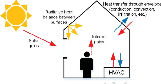
(ASHRAE 2009) to simulate a series of phenomena, including heat conduction through the building envelope, convection between internal surfaces and the air, radiative heat transfer, infiltration and contributions from the HVAC system (see Figure 1). To use this white-box approach, a detailed knowledge of the building is required, which is unfortunately not always available.
INSERT FIGURE 1 HERE
Figure 1. Simplified heat balance representation in buildings
Unlike white-box models, black-box models do not perform energy analysis and do not require detailed building characteristics; instead, they learn from historical data to make predictions using machine learning algorithm (Amasyali and Gohary 2018). According to Amasyali and El-Gohary (2018), the development of a black-box model is composed of four steps: data collection, data preprocessing, model training and model testing. More than sixty studies on the use of black-box models for building energy consumption prediction are reviewed by Amasyali and El-Gohary (2018). Among them, 47 % use artificial neural networks, 25 % support vector machines, 4 % decision trees, and the remaining 24 % use other statistical methods such as multiple linear regression, ordinary least squares regression and autoregressive integrated moving average methods. As highlighted by these numbers, neural network (NN) models are popular black-box modeling methods used to tackle complex and ill-defined problems. Among these NN models, a particular type known as “autoregressive NN with exogenous variables” (NNARX) is well adapted for energy consumption and temperature prediction, using historical and present values of input and output variables as inputs to forecast future conditions. NNARX models are a type of non-linear autoregressive techniques with exogenous inputs (NARX). Bennett, Stewart and Lu (2014) compared the use of time series techniques (e.g., autoregressive integrated moving average with
exogenous variables ARIMAX) and NN models to forecast the next day total energy use and peak demand on the electric network, using historical values as inputs. In this study, the NN models performed slightly better than the ARIMAX method. Hybridization of both methods was also successfully tested. Ruiz et al. (2016) proposed to use non-linear autoregressive neural networks with and without exogenous inputs to predict future energy consumption. Their models were applied to public buildings and the comparison with experimental results showed that using exogenous inputs increases the accuracy significantly. Autoregressive NN models are also used for temperature prediction. Kramer, van Schijndel and Schellen (2012) reviewed simplified thermal building models, including a NNARX model for temperature prediction in buildings. Frausto and Pieters (2004) modeled a greenhouse with autoregressive NN using the outside air temperature, humidity, solar radiation and sky cloudiness to predict the indoor temperature. This study followed previous work using time series techniques to carry out the same objective (Frausto, Pieters, and Deltour 2003). Time series models were not able to predict correctly the greenhouse indoor temperature due to their inability to consider non-linearities. This observation was confirmed by Mechaqrane and Zouak (2004) and by Mustafaraj, Lowry and Chen (2011), who compared linear and neural network-based autoregressive models with exogenous inputs (outside temperature, solar radiation and heating power) to predict the indoor temperature of residential and office buildings. The exogenous inputs included the outside temperature, solar radiation and heating power for the first reference (Mechaqrane and Zouak 2004), and the outside temperature, outside relative humidity, room temperature, room relative humidity, supply air temperature, supply air relative humidity, supply air flow-rate, chilled water temperature (from cooling system), hot water temperature (from heating system) and room carbon dioxide concentration for the second reference (Mustafaraj et al. 2011). For both references, the NNARX model outperformed the linear
ARX model, showing that the NN models captured non-linearities. By considering past values, NNARX models look like recurrent neural networks (RNN), which include state variables that store past information (Zhang et al. 2019), making RNN appropriate to handle sequential information or time series. Unlike RNN, NNARX models have a feedback coming only from the output neuron rather than from the hidden states (Siegelmann et al. 1997). Siegelmann, Horne and Giles (1997) indicated that NNARX models are more efficiently trained (Horne and Giles 1995) and perform better on problems involving long-term dependencies (Lin et al. 1996), compared to RNN.
An intermediate solution between white-box and black-box approaches is gray-box modeling. Gray-box models are reduced or low-order models that are well documented in the literature, especially for simplified building energy simulation. They can take different designations, such as state-space models (Hu and Karava 2014), lumped parameters models (Ramallo-González et al. 2013), gray-box models (Braun and Chaturvedi 2002), thermal network models (Xu and Wang 2008) and resistance-capacitance (RC) models (Bueno et al. 2012). The core idea is to apply the principle of inverse modeling (Nakamura and Potthast 2015), defining a physics-based model where unknown parameters are identified by optimization (minimization of differences between simulated and experimental results).
Key end applications of simplified building models (black-box and gray-box) include improved control of building mechanical components, e.g., HVAC systems, and automated fault detection and diagnosis, leading to optimized energy use, thermal comfort and financial costs. Afram and Janabi-Sharifi (2014) reviewed model predictive control (MPC) applied to HVAC systems, presenting in details this approach and comparing it to other control methods (e.g., classical, hard, soft and hybrid). If properly developed and implemented, MPC has the potential to reduce energy
consumption (Oldewurtel et al. 2010) and to improve thermal comfort (Castilla et al. 2014) inside buildings, compared to traditional rule-based controllers. In terms of fault detection and diagnosis (FDD), Katipamula and Brambley (2005a, 2005b) wrote a two-part review about FDD methods applied to HVAC systems. Among the different methodologies reviewed in this paper, process history-based methods require the use of black-box or gray-box models to perform automated FDD. This review was recently updated (Kim and Katipamula 2018), highlighting in the conclusion the fact that process history-based (i.e., data-driven) methods are most commonly used. Kim and Katipamula (2018) also indicated an interesting figure: nearly 30 % of the energy consumption in commercial building (HVAC and lighting) is caused by inadequate sensing and controls, and by the inability to properly use the capabilities of existing building automation systems.
In North America, the most commonly used space heating and cooling systems for small commercial buildings are rooftop units (RTUs). Typically, RTU include a gas-powered heating system and a vapor compression cycle for cooling (Djunaedy et al. 2011). In the U.S., RTUs were used in 2015 in 46 % of all commercial buildings, representing around 60 % of the commercial building floor space and around 2.6 quads annually of primary energy consumption (Katipamula et al. 2015). Thereby, a gain in energy efficiency for these systems can lead to a significant reduction in energy consumption for the commercial building sector. If equipped with appropriate sensors generating a large quantity of data, RTUs could work more efficiently by processing and exploiting this data to improve control strategies and FDD, leading to higher energy efficiency and thermal comfort. Doing so requires the development of models capable of predicting accurately the behavior of buildings.
2. Problem Statement and Objectives
When HVAC automation engineers implement a new control system in a building, the characteristics of the building (envelope, HVAC system, etc.) are rarely known in detail. They initially implement traditional rule-based controllers. Over time, more data are collected, such as zone temperatures and energy use. When enough data is obtained, a data-driven control system can be developed, tested and deployed, leading to improved building operations. This system should be based on a black-box model capable of simulating and predicting accurately the building’s thermal behavior, leading to wise and proactive control decisions. Unfortunately, the quality and quantity of available data often do not match the requirements needed to develop accurate black-box models, preventing their use to improve the building operations. In the introduction, the presented applications use extensive datasets to develop black-box models for indoor temperature predictions in buildings, including the indoor / outdoor temperature, solar radiation, heating power, indoor / outdoor relative humidity, etc. In the application presented in this paper, the dataset is more limited and is composed of different kind of data, as presented in the following section. The challenge is to exploit the available data to develop accurate black-box models. More specifically, the objectives of this work are:
- To develop a methodology leading to the development of ܰ௧-order autoregressive neural
networks with exogenous inputs (NNARX models) for indoor temperature prediction in buildings. The “ܰ௧-order” means that data from ܰ previous time-step(s) (including current
time) are used to forecast the next time-step. In contrast with references (Mechaqrane and Zouak 2004; Frausto and Pieters 2004; Mustafaraj et al. 2011) presented in the introduction, we develop a method leveraging occupancy and time-related data without considering solar radiation and relative humidity.
- To compare this NN model with alternative models, i.e., a gray-box model and black-box linear models (i.e., ARX models).
- To verify the accuracy of the models when running in a real simulation mode, considering error propagation with time.
The proposed methodology is validated using real data obtained from an existing commercial building in Montreal (QC, Canada). This application is discussed in detail in the following section, with a particular focus on the data description and pre-processing. Section 4 focuses on the methodologies of the modeling approaches considered in this study. For each of them, a mathematical formulation is given, and the treatment of inputs and outputs is presented. Section 4 also discusses the error indicators applied in this study. In Section 5, we discuss the results of the different models and compare their accuracy.
The novelty of this study is double in terms of contributions: first, to bridge a knowledge gap related to the composition of the dataset needed to obtain an effective black-box model; secondly, to emphasize the loss in accuracy due to error propagation when a trained model is used to predict indoor temperatures in buildings.
Compared to the cases considered in the literature review, the composition of the available dataset is different. In the literature, the data used in black-box models is usually the inside and outside temperatures, solar radiation, indoor and outdoor humidity, heating power, etc. In the case presented in this paper, the available data is more limited: solar radiation, indoor and outdoor humidity are for example not available. This lower quantity of available data introduces a potential gap in terms of performance of the model to forecast indoor temperatures in buildings.
3. The second contribution of this study is to highlight the impact of the error propagation on the accuracy of predictions when using trained black-box models. This information is rarely provided in the literature, while this gap in accuracy is a key challenge.Application and Data Description
Throughout the paper, the methodology is illustrated with an application to a commercial building (large open space used as a retail shop) of around 1000 m2located in Montreal (QC, Canada) and
equipped with three RTUs providing space heating and cooling. RTUs are controlled individually based on signals from three thermostats located at three different locations in the open space. Both heating and cooling systems can be operated at two power levels: first stage heating ܲ,௦ଵ = 39.8 kW; second stage heating ܲ,௦ଶ= 59.8 kW; first stage cooling ܲ,௦ଵ= 18.5 kW; second stage cooling ܲ,௦ଶ = 37 kW. The second stage always works with the first stage (i.e., ܲ,௦ଵ+ ܲ,௦ଶ in heating or ܲ,௦ଵ+ ܲ,௦ଶ in cooling), while the first stage can operate alone. Each RTU is also equipped with a 1.4 kW fan activated whenever the heating or cooling system is on.
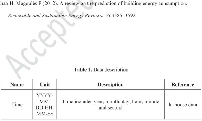
Table 1 presents all the data used in this work. They were collected in the winter season, which explains the absence of cooling stages in the table. The considered period ranges from December 13, 2018 (00:00) to January 22, 2019 (23:59), i.e., around 1000 hours. Data was acquired with a 5-minute time-step. Aside from in-house data collected every five minutes on site, data described in Table 1 come from two other sources: the outside temperature from the Dark Sky weather API (Hernandez 2019; The Dark Sky Company 2019); and the occupancy data from the Google Popular Times API (Anonymous 2019; Google 2019). These two sources provide hourly measurements. Interpolation is then carried out to obtain a full dataset with a constant time interval of five minutes. Step interpolation technique (using previous values) is utilized for binary variables (ON/OFF), while linear interpolation is applied to continuous variables, i.e., temperatures in this
case. Compared to the references (Mechaqrane and Zouak 2004; Frausto and Pieters 2004; Mustafaraj et al. 2011) presented in the introduction, two major features are not available in this application: solar radiation and indoor / outdoor relative humidity.
Table 1. Data description INSERT TABLE 1 HERE
For black-box models, an important data pre-processing step consists in normalizing the empirical distribution of each variable so that it has a mean of zero and a standard deviation of one. Zhang, Patuwo and Hu (1998) examined and confirmed the usefulness of data normalization to train neural networks more efficiently. In this study, the normalized data are computed using the empirical arithmetic mean ߤ and the empirical standard deviation ߪ of each variable ݔ, as presented in the following equations: ߤ =1 ݊ ݔ ୀଵ (1) ߪ = ඩ1 ݊ (ݔെ ߤ) ଶ ୀଵ (2)
The full dataset consists of nearly 1000 hours of measurements with a five-minute time-step, i.e., around 12000 data points. Black-box and gray-box models need data to be trained and cannot be validated using the same dataset. Thus, the full initial dataset is divided in two parts: one for training (from December 13, 2018 at 00:00 to January 15, 2019 at 23:59) and one for testing (from January 16, 2019 at 00:00 to January 22, 2019 at 23:59). In the specific case of neural networks, three datasets are defined: the training dataset is the same as previously defined; the validation dataset is randomly chosen among the training dataset (20 % of the training dataset) to improve the training and to avoid overfitting; the testing dataset is similar to the one previously defined.
4. Modeling Methodologies
This section describes the modeling approaches (gray-box, ARX and NNARX models) applied in this work, and the indicators used to quantify the model errors and to compare the different approaches.
4.1 Gray-box Modeling Method
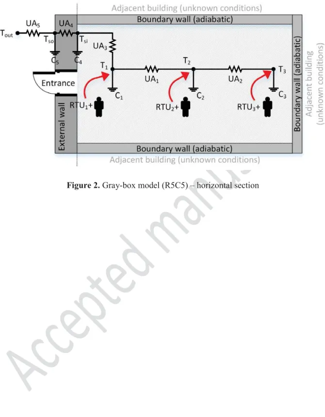
Figure 1 illustrates the energy balance observed in buildings. However, details needed to model it are often missing. In the present application (see section 3), many details are unknown, e.g., the exact geometry of the building, its envelope, the solar gains and the internal gains (e.g., heat dissipation from equipment). A simplified thermal resistance-capacitance (RC) model may then be developed to model the building, as shown in Figure 2. As presented in this figure, the building is surrounded by other buildings and only the wall with the entrance is external. The only known boundary condition is the outside temperature ܶ௨௧. Adiabatic boundary conditions are assumed for adjacent buildings. Surface temperatures ܶ௦and ܶ௦are also unknown but are needed since the impact of the wall thermal mass is high and must therefore be defined. The model is composed of 5 resistances (defined as global heat transfer coefficients ܷܣ [in W/K]), 5 state variables (temperatures ܶଵ, ܶଶ, ܶଷ, ܶ௦and ܶ௦) and 14 inputs (1 for outside temperature ܶ௨௧, 1 for occupancy and 12 for RTU configurations for the 3 zones). As the only windows are oriented to the north-west (external wall), it is assumed that solar radiation does not impact significantly the energy balance inside the building and solar gains are thus assumed to be negligible. Another reason to assume no solar radiation is the lack of field data of this feature.
INSERT FIGURE 2 HERE
Figure 2. Gray-box model (R5C5) – horizontal section
ܶሶଵ =ܷܣଵ ܥଵ (ܶଶെ ܶଵ) + ܷܣଷ ܥଵ (ܶ௦െ ܶଵ) + ܲ,௦ଵ,௭ଵ ܥଵ ܿݏ,௦ଵ,௭ଵ+ ܲ,௦ଶ,௭ଵ ܥଵ ܿݏ,௦ଶ,௭ଵ െܲ,௦ଵ,௭ଵ ܥଵ ܿݏ,௦ଵ,௭ଵെ ܲ,௦ଶ,௭ଵ ܥଵ ܿݏ,௦ଶ,௭ଵ+ ܲ,௫,௭ଵ ܥଵ ܱܿܿ (3) ܶሶଶ = ܷܣଵ ܥଶ (ܶଵെ ܶଶ) + ܷܣଶ ܥଶ (ܶଷെ ܶଶ) + ܲ,௦ଵ,௭ଶ ܥଶ ܿݏ,௦ଵ,௭ଶ+ ܲ,௦ଶ,௭ଶ ܥଶ ܿݏ,௦ଶ,௭ଶ െܲ,௦ଵ,௭ଶ ܥଶ ܿݏ,௦ଵ,௭ଵെ ܲ,௦ଶ,௭ଶ ܥଶ ܿݏ,௦ଶ,௭ଶ+ ܲ,௫,௭ଶ ܥଶ ܱܿܿ (4) ܶሶଷ = ܷܣଶ ܥଷ (ܶଶെ ܶଷ) + ܲ,௦ଵ,௭ଷ ܥଷ ܿݏ,௦ଵ,௭ଷ+ ܲ,௦ଶ,௭ଷ ܥଷ ܿݏ,௦ଶ,௭ଷെ ܲ,௦ଵ,௭ଷ ܥଷ ܿݏ,௦ଵ,௭ଷ െܲ,௦ଶ,௭ଷ ܥଷ ܿݏ,௦ଶ,௭ଷ+ ܲ,௫,௭ଷ ܥଷ ܱܿܿ (5) ܶሶ௦ =ܷܣଷ ܥସ (ܶଵെ ܶ௦) + ܷܣସ ܥସ (ܶ௦െ ܶ௦) (6) ܶሶ௦= ܷܣସ ܥହ (ܶ௦െ ܶ௦) + ܷܣହ ܥହ (ܶ௨௧െ ܶ௦) (7)
or equivalently, in the following matrix form (Myers 1971):
ܶሶଵ ڭ ܶሶ௦ = [ܣ] ܶଵ ڭ ܶ௦ ൩ + [ܤ] ቈ ܿݏ,௦ଵ,௭ଵ ڭ ܱܿܿ (8)
Matrices ܣ and ܤ (5-by-5 and 5-by-14, respectively) in Eq. (8) are defined by 13 parameters, which must be identified. These parameters are the 5 coefficients ܷܣ, the 5 capacitances ܥ and the 3 maximum occupancy-related heat gains ܲ,௫, defining the heat gains related to the maximum recorded occupancy for each zone. An optimization algorithm is applied to identify the parameter values minimizing the root mean square deviation between observed and simulated temperatures. In this work, this state-space model is solved using the SciPy Python library (The SciPy community 2019).
4.2 Black-box Linear Models
We consider now a black-box linear model taking the form of an autoregressive model with exogenous variables (ARX), whose goal is to forecast outputs of interest. This model aims at predicting the vector of future temperatures ܶ௧ାο௧based on past and current values of temperatures (autoregressive terms ܶ) and other exogenous inputs ܺ, detailed below. This model may be mathematically formulated as a general linear model (Kutner et al. 2005):
ܶ௧ାο௧ = ݓ௧ିο௧, ܶ௧ିο௧, ୀଵ ே ୀ + ݓ௧ିο௧, ܺ௧ିο௧, ୀଵ ே ୀ (9)
where ܰ is the number of past time-steps considered (order of autoregressive models); ்݊ and ݊ are the number of autoregressive and exogenous terms; and ݓ are the weights.
Unlike neural networks, ARX models are linear and therefore cannot capture non-linearities such as radiative heat transfer in buildings. The weights for each input variables (autoregressive and exogenous) are identified using the training dataset and the ordinary least squares (OLS) algorithm (Kutner et al. 2005). In this study, the tool used to achieve this work is an OLS linear regression function from the Scikit-learn python library (Scikit-learn 2019a, Pedregosa et al. 2011).
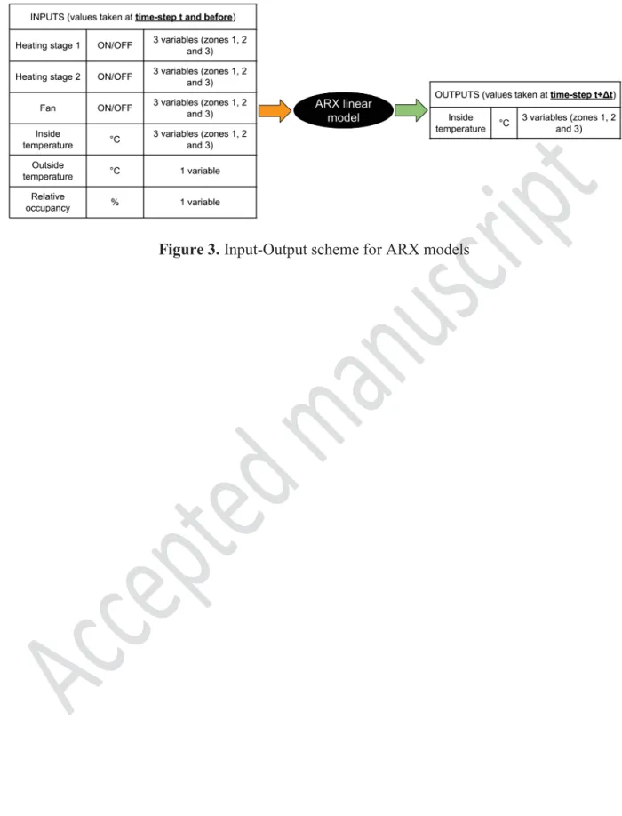
Figure 3 presents the inputs and outputs used in this approach. Inside temperatures are the autoregressive terms, while relative occupancy, outside temperature and control signals (ON/OFF) from heating stages and fans are the exogenous terms. The number of previous time-steps considered changes depending on the order. In this work, three orders are tested: 1st (last 5
minutes), 6th(last 30 minutes) and 12th(last hour).
INSERT FIGURE 3 HERE
4.3 Neural Network Models
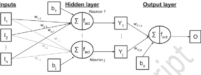
Neural networks (Davalo and Naïm 1991; Hagan et al. 1996) consist of a network of processing units, called “neurons”, whose purpose is to establish mathematical relationships between input and output data. Each neuron performs simple computation tasks that may be formulated as follows: ܻ = ݂௧ቌܾ + ݓ ܫ ୀଵ ቍ (10)
where ܻ is the neuron’s output; ܾ is a constant bias associated to a neuron; ݊ is the number of inputs; ݓ are the weights; ܫ are the inputs (autoregressive or exogenous term); ݂௧is the activation function.
The activation function ݂௧ (Zhang et al. 2019a) processes the outcome of the weighted sum
carried out by a neuron. Examples of commonly used activation functions are the rectified linear unit (ReLU), sigmoid or hyperbolic tangent functions. These functions can handle non-linearities. The association of neurons produces a NN, which is composed of two or more neuronal layers. Figure 4 presents a simple case with two layers: one hidden layer with ݆ neurons processing ݊ inputs and one output layer yielding the output ܱ from the outputs ܻ of the previous stage.
Training NNs means optimizing the weights ݓ and bias ܾ, associating the input and output vectors, and minimizing the errors between predicted and observed output values.
INSERT FIGURE 4 HERE
Figure 4. Neural network with ݊ inputs ܫ, 1 hidden layer with ݆ neurons and one output ܱ Another well-known term used in the literature to designate a NN is multi-layer perceptron (MLP) (Scikit-learn 2019c; Zhang et al. 2019a).
In this work, MLPs are trained to forecast zone temperatures at time-step ݐ + οݐ from conditions at time-step ݐ, using the MLPRegressor class in the Scikit-Learn library (Scikit-learn 2019c, Pedregosa et al. 2011).
The size of a MLP model mainly depends on the number of inputs, outputs, and samples. Bigger buildings generally generate higher numbers of inputs, outputs, and samples, which lead to neural networks with a higher number of hidden neurons. Unfortunately, there is no scientific consensus on how to define the number of hidden neurons in neural networks. Sheela and Deepa (2013) reviewed 101 techniques to define the number of hidden neurons based on the number of inputs, outputs, and samples. They applied these techniques to a specific case, and the number of hidden neurons varied in the range 100:1. As indicated by Sheela and Deepa (2013), there is then no generally accepted theory to define the number of hidden neurons. On the other hand, there is a consensus on another aspect: a neural network with a high number of neurons leads to longer computation times and overfitting. In our case, both of these issues are minimized. Computation time is in this case not an issue because the defined neural networks are small (maximum 400 neurons), compared to applications like computer vision that requires deep neural networks. Overfitting is also avoided because the dataset is divided (training, validation and testing) and an early stopping technique is used. In the literature, early stopping is well recognized to be an effective approach to avoid overfitting (Prechelt 1998; Caruana et al. 2001). For the targeted application (to forecast indoor temperatures in buildings), references from the literature use a number of hidden neurons generally around 10-20 neurons. We have chosen to use 2 configurations in our case: 10 neurons (2 hidden layers of 5 neurons) and 400 neurons (2 hidden layers of 200 neurons). The first configuration is in line with the references, while the second
configuration with 400 neurons has been chosen to verify that overfitting was well mitigated with techniques like the dataset division (training, validation, and testing) and early stopping.
The chosen activation function is ReLU, the solver selected for training of the MLP is Adam (Zhang et al. 2019b) and the early stopping function is activated using a 20 % validation dataset (randomly chosen in the training dataset) to avoid overfitting.
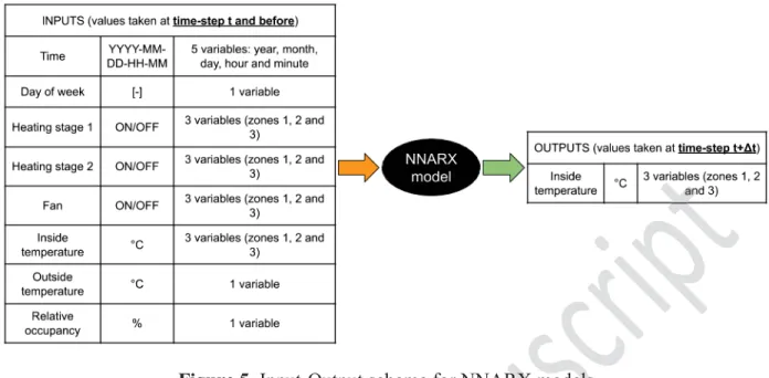
Figure 5 presents the inputs (20) and outputs (3) considered in autoregressive NN models with exogenous inputs, i.e. NNARX models.
INSERT FIGURE 5 HERE
Figure 5. Input-Output scheme for NNARX models
Compared to black-box linear models (see Figure 3), the time and day of the week are given to the NNARX models. These data can provide additional insight about the occupancy and thermal gains (internal and solar mainly) in the building, which can be captured by NN models (unlike linear models). For example, the hour of the day gives a non-linear indication about the solar position and the occupancy of a building. As for the previous linear models, the number of previous time-steps considered changes depending on the defined order. The same three orders are tested, i.e., 1st
(last 5 minutes), 6th(last 30 minutes) and 12th(last hour).
4.4 Error Indicators
Amasyali and El-Gohary (2018) reviewed many indicators used to evaluate the performance of data-driven models of buildings. Among them, three are considered in this study: the coefficient of determination ܴଶ, the root mean square error ܴܯܵܧ and the normalized mean bias error ܰܯܤܧ.
ܴଶ is an indicator of how well observed outputs are replicated by the model. The closer to a value of one, the better it is. It is computed as follows:
ܴଶ = 1 െσ ൫ܶ െ ܶ൯ ଶ ୀଵ σ (ܶെ ܶത)ଶ ୀଵ (11)
Where ݊ is the number of samples; ܶ is the observed value; ܶ is the predicted value; ܶത is the average of observed values.
ܴܯܵܧ is a measure of the average deviation observed between actual and predicted values. This indicator is expressed in the same unit as the outputs of interest, i.e., in degree Celsius in this work. ܴܯܵܧ is defined as follows: ܴܯܵܧ = ඨσ ൫ܶ െ ܶ൯ ଶ ୀଵ ݊ (12)
Finally, ܰܯܤܧ is an adequate indicator to evaluate if the model globally over- or under-estimates the observed values. If positive, the model overestimates the reality. In Section 5, the absolute value of ܰܯܤܧ, i.e., |ܰܯܤܧ|, is often used. ܰܯܤܧ is expressed in percentage and is calculated as follows:
ܰܯܤܧ =σ ൫ܶ െ ܶప ൯
ୀଵ
݊ ܶത × 100 (13)
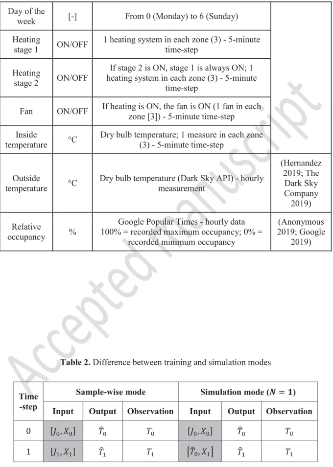
For black-box models (ARX and NNARX), the error is evaluated differently depending on how the model is used, i.e., in a sample-wise or an actual simulation mode. Table 2 illustrates this difference.
Table 2. Difference between training and simulation modes INSERT TABLE 2 HERE
When the model is applied individually to each data sample, the error is evaluated in a sample-wise manner, considering the inputs (autoregressive and exogenous terms ܬ and ܺ) and outputs provided by the training dataset. When the model is deployed in simulation mode, the inputs include, after the initial time-step 0 (initial conditions), the exogenous terms ܺ (as in training) and the previous predicted output(s) ܶ (unlike in training), leading to a propagation of error over time.
5. Results and Discussion
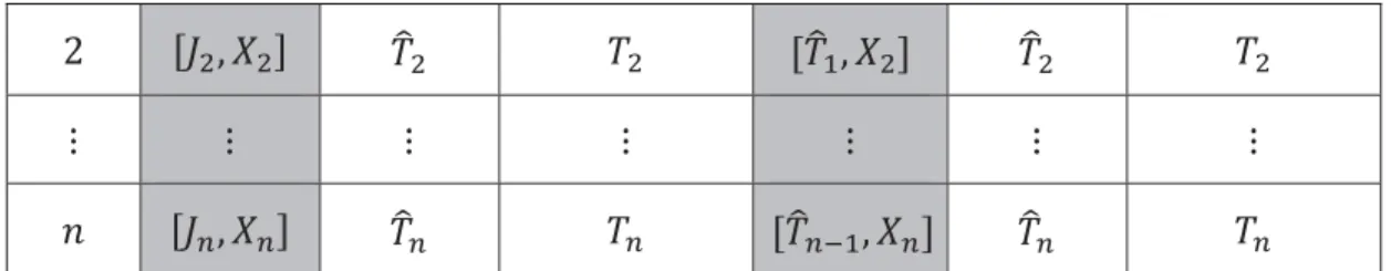
The discussion of the main results is organized in three steps: first, the global comparison of all the models; second, the presentation of results in simulation mode for the most accurate model family; finally, a comparison of results in simulation mode between the best models of each family. Table 3 presents the values of each error indicator (ܴଶ, ܴܯܵܧ and ܰܯܤܧ) given for each model,
each dataset (training and testing) and each mode (sample-wise and simulation). The sample-wise mode is not available for the gray-box R5C5 model because this mode is never used for this model (see section 4.4).
Table 3. Results summary INSERT TABLE 3 HERE
A first obvious observation valid for all models is the decrease in accuracy when the dataset or the mode is switched from training to testing or from sample-wise to simulation, respectively.
The gray-box R5C5 model has a significantly lower accuracy (low ܴଶ, and high ܴܯܵܧ and
|ܰܯܤܧ|), compared to the best ARX and NNARX models. Like white-box models, gray-box modeling still depends on a knowledge of the building characteristics. In this work, this information is lacking, which penalizes the accuracy of the gray-box model. An underlying consequence is the inability to model some phenomena impacting the thermal behavior of the
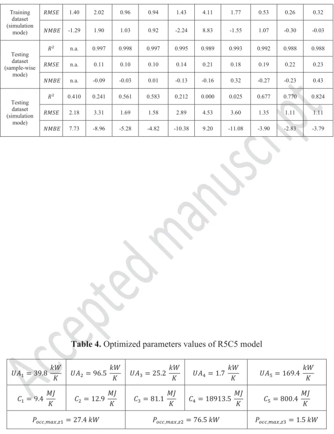
building, e.g., the heat transfer between the adjacent buildings and the building of interest. This difficulty also appears when the results of the model calibration are analyzed. The 13 parameters of the gray-box model have been identified by minimizing the ܴܯܵܧ between observed and simulated temperature values (training dataset), leading to optimized values presented in Table 4. Some of them have irregularities, especially the ܲ,௫values which characterizes the maximum occupancy-related heat gains in each zone of the building. The high values for zones 1 and 2 are probably caused by the inclusion of the internal gains from devices or solar gains. The low value obtained for zone 3 might be explained by its location (see Figure 2 in section 4.1), the farthest from the entrance (and so, from solar radiation) and surrounded by adiabatic boundary conditions minimizing artificially heat losses and the ܲ,௫,௭ଷvalue. In brief, the R5C5 model results show
that physics-based models (white-box or gray-box) may be inadequate in the specific situation where information about the building characteristics is insufficient.
Table 4. Optimized parameters values of R5C5 model INSERT TABLE 4 HERE
As for the black-box models, all ARX and NNARX models perform relatively well in sample-wise mode using the training dataset, producing low ܴܯܵܧ and |ܰܯܤܧ|, and high ܴଶ (see Table
3). The training results are also validated with the testing dataset in sample-wise mode, where the errors have approximately the same order of magnitude as for the training dataset. These results indicate that the list of features used as inputs (see Figures 3 and 5) are sufficient to explain the variations of indoor temperatures in each zone, and that overfitting was correctly mitigated. However, a training validated by a testing dataset does not necessarily lead to effective prediction in simulation mode. The best way to evaluate a trained model is to apply it in a real deployment configuration, i.e., in simulation mode. When doing so, clear differences are highlighted: the
ARX(1) model and all NNARX models with 2 × 5 neurons yield relatively high inaccuracies, while the other models (ARX(6), ARX(12) and all NNARX with 2 × 200 neurons) produce acceptable results. The poor performance of all NNARX models with 2 × 5 neurons is due to the inability of a relatively small NN to capture the whole complexity of the information provided in the training dataset. With the testing dataset, acceptable models produce ܴଶ above 0.55 (up to
0.824), ܴܯܵܧ lower than 1.70 °C (down to 1.11 °C) and |ܰܯܤܧ| lower than 6 % (down to 2.83 %). These results are given for a whole week with a 5-minute time-step. Another aspect highlighted by the switch from sample-wise mode to simulation mode is the interest of increasing the number ܰ of past values (increasing the number of inputs) to increase the accuracy of the models. For example, for NNARX models with 2 × 200 neurons, increasing ܰ changes ܴଶ from
0.677 to 0.824 when considering the testing dataset.
Table 3 also indicates that the best model family in terms of accuracy is the NNARX models with 2 × 200 neurons. Figure 6 compares the experimental results with the simulated results obtained with these NNARX models for the first 50 hours of the testing dataset in simulation mode and for each zone of the building. During this period, the temperature setpoint changes from ~21 °C during the daytime to ~16 °C overnight. All experimental temperature curves follow the same trend in all three zones. The results show that all NNARX models perform in a similar way with few differences observed between them. Differences are clearer over a longer period, such as presented in Table 3. For all NNARX models, the highest differences between experimental and simulated results are observed during the daytime, caused by the absence of solar radiation data in the inputs. Gaps are especially noticeable during the second day (between the 30th and 45thhours) in zone 1
and during both days (between the 5thand 15thhours, and between the 35thand 45thhours) in zone
Depending on the periods, some NNARX models can be less accurate than the others. For examples, the NNARX(1), NNARX(6), and NNARX(12) models are the least accurate during the period between the 45th and 50thhours in zone 2, between the 45th and 50thhours in zone 3, and
between the 23rdand 28thhours in zone 3, respectively.
After 50 hours, all models display a ܴܯܵܧ of around 0.6 °C (i.e., around half than the lowest ܴܯܵܧ observed in Table 3 after a 1-week simulation with the testing dataset), as shown in Figure 6(d). It must be noted that, when predictive control is sought, the model precision during the first few hours is the most important. Moreover, the precision of temperature sensors is often around ± 0.5 °C, this value being an appropriate benchmark for the accuracy of models. Therefore, these NNARX models can be considered accurate for this time horizon.
INSERT FIGURE 6 HERE
Figure 6. Comparison of the experimental results with the results obtained with the NNARX models (2 × 200 neurons) from January 16, 2019 at 00:00 to January 18, 2019 at 02:00 As shown in Table 3 for the testing dataset in simulation mode, the best ARX and NNARX models are ARX(12) and NNARX(12) (NNARX(6) is also very close). Figure 7 compares both models over the first 50 hours of the testing dataset in simulation mode in zone 2 only. As observed in Figure 6, all zones behave in the same way. For additional comparison, the results of the gray-box R5C5 model are also presented.
As the results of Table 3 suggested, both black-box models outperform the gray-box model, which is not capable of replicating the temperature variations. For the gray-box model, the difference between experimental and simulated temperatures can reach up to 2 °C (observed at the 10thhour).
a minimum of ~19 °C and a maximum of ~24 °C, while the experimental values are approximately between ~18 °C and ~22 °C.
As for the black-box models, both ARX(12) and NNARX(12) models generate accurate and similar results. However, several periods highlighted by gray circles in Figure 7 show that the NNARX model is significantly more accurate, especially in two situations: first, the decrease in temperature after the setpoint change (see the time intervals [0, 5] and [45, 50]); second, the higher temperatures experienced during the daytimes (see the time intervals [15, 20] and [30, 40]). The lower accuracy of the ARX model may be caused by its linear nature. Unlike NNARX models, ARX models cannot model non-linearities such as radiative heat transfer or occupancy-related heat gains.
INSERT FIGURE 7 HERE
Figure 7. Comparison of the experimental results with the results obtained with the R5C5, ARX(12) and NNARX(12) (2 × 200 neurons) models for zone 2 from January 16, 2019 at 00:00
to January 18, 2019 at 02:00
6. Conclusion
The present work is dedicated to the development of autoregressive neural networks with exogenous variables (NNARX) for predicting indoor temperatures in buildings. A comparison with alternative models, i.e., a gray-box resistance-capacitance model and black-box autoregressive linear models (ARX), is also presented. The methodology is applied to an existing commercial building in Montreal (QC, Canada) operating in winter conditions. Available experimental data include autoregressive terms, i.e., the indoor temperatures of each zone (3), and exogenous inputs, i.e. the time, day of the week, heating stages (ON/OFF), fan (ON/OFF), outside
temperature and relative occupancy. Compared to other cases found in the literature, key data are not available, including solar radiation, and indoor / outdoor humidity.
The lack of information about the characteristics of the building prevents the gray-box R5C5 model to perform accurately and highlights the interest for an effective purely data-driven (black-box) model. Results show that both ARX and NNARX models can perform adequately under certain conditions. ARX models need more past terms (6th- and 12th-order models ARX(6) and
ARX(12)) to perform well while the differences in performance between NNARX models (1st-,
6th- and 12th-order) are much lower. The performance of NN models depends on the number of
neurons, defining their ability to capture the information of interest in the data. Thereby, the NN configuration with 2 × 200 neurons outperforms the other architecture with only 2 × 5 neurons. An important aspect to highlight is the fact that this difference in performance is not visible when looking at the training phase and its validation with the testing dataset using a sample-wise mode. This difference becomes clearly noticeable when the NN models are used in a simulation mode, taking previous guessed values to predict the next value, i.e., considering the error propagation. A comparison between the best ARX and NNARX models (12th-order) shows a slight superiority of
the NNARX model, which is helped by its ability to consider non-linearities. In simulations with the full testing dataset (one full week with a 5-minute time-step), the NNARX(12) model produces low error (ܴଶ = 0.824; ܴܯܵܧ = 1.11 °C; ܰܯܤܧ = -3.79 %), while the ARX(12) model yields
higher error (ܴଶ= 0.583; ܴܯܵܧ = 1.58 °C; ܰܯܤܧ = -4.82 %). These errors can be considerably
reduced if a shorter time horizon is chosen. For example, a 50-hour time horizon leads to a ܴܯܵܧ of 0.6 °C for the best NNARX models. This value should be compared to the precision of most temperature sensors, i.e., around ± 0.5 °C. The 50-hour time horizon is also appropriate when predictive control is sought.
Further research will lead to the integration of NNARX models for indoor temperature prediction in different applications such as model predictive control or automated fault detection and diagnosis.
References
Afram A, Janabi-Sharifi F (2014). Theory and applications of HVAC control systems – A review of model predictive control (MPC). Building and Environment, 72:343–355.
Amasyali K, El-Gohary NM (2018). A review of data-driven building energy consumption prediction studies. Renewable and Sustainable Energy Reviews, 81:1192–1205.
Anonymous (2019). Populartimes. Available at: https://github.com/m-wrzr/populartimes. Accessed 8 Feb 2019.
ASHRAE (2009). Heat balance method. In: 2009 ASHRAE Handbook - Fundamentals (SI Edition). American Society of Heating, Refrigerating and Air-Conditioning Engineers, Atlanta, GA, USA, pp 18.15-18.18.
Beckman WA, Broman L, Fiksel A, et al (1994). TRNSYS The most complete solar energy system modeling and simulation software. Renewable energy, 5:486–488.
Bennett C, Stewart AR, Lu J (2014). Autoregressive with Exogenous Variables and Neural Network Short-Term Load Forecast Models for Residential Low Voltage Distribution Networks. Energies, 7(5):2938–2960.
Braun JE, Chaturvedi N (2002). An Inverse Gray-Box Model for Transient Building Load Prediction. HVAC&R Research, 8:73–99.
Bueno B, Norford L, Pigeon G, Britter R (2012). A resistance-capacitance network model for the analysis of the interactions between the energy performance of buildings and the urban climate. Building and Environment, 54:116–125.
Caruana R, Lawrence S, Giles CL (2001). Overfitting in neural nets: Backpropagation, conjugate gradient, and early stopping. In: Advances in neural information processing systems,
pp.402–408.
Castilla M, Álvarez JD, Normey-Rico JE, Rodríguez F (2014). Thermal comfort control using a non-linear MPC strategy: A real case of study in a bioclimatic building. Journal of Process Control, 24:703–713.
Coakley D, Raftery P, Keane M (2014). A review of methods to match building energy
simulation models to measured data. Renewable and Sustainable Energy Reviews, 37:123–
141.
Crawley DB, Hand JW, Kummert M, Griffith BT (2008). Contrasting the capabilities of building energy performance simulation programs. Building and Environment, 43:661–673.
Crawley DB, Lawrie LK, Winkelmann FC, et al (2001). EnergyPlus: creating a new-generation building energy simulation program. Energy and Buildings, 33:319–331.
Davalo E, Naïm P (1991). Neural Networks. Paris, France: Macmillan Education.
Djunaedy E, van den Wymelenberg K, Acker B, Thimmana H (2011). Oversizing of HVAC system: Signatures and penalties. Energy and Buildings, 43:468–475.
Foucquier A, Robert S, Suard F, et al (2013). State of the art in building modelling and energy performances prediction: A review. Renewable and Sustainable Energy Reviews, 23:272–
288.
Frausto HU, Pieters JG (2004). Modelling greenhouse temperature using system identification by means of neural networks. Neurocomputing, 56:423–428.
Frausto HU, Pieters JG, Deltour JM (2003). Modelling Greenhouse Temperature by means of Auto Regressive Models. Biosystems Engineering, 84:147–157.
Google (2019). Popular times, wait times, and visit duration. Available at:
https://support.google.com/business/answer/6263531?hl=en. Accessed 8 Feb 2019. Hagan MT, Demuth HB, Beale MH, De Jesús O (1996). Neural Network Design. Boston, MA:
PWS Publishing Company.
Hand JW (2011). The ESP-r cookbook. University of Strathclyde, Glasgow, Scotland. Hernandez A (2019). A Python wrapper for the forecast.io API. Available at:
https://github.com/bitpixdigital/forecastiopy3. Accessed 8 Feb 2019.
Horne BG, Giles CL (1995). An experimental comparison of recurrent neural networks. In: Advances in neural information processing systems. pp 697–704.
Hu J, Karava P (2014). A state-space modeling approach and multi-level optimization algorithm for predictive control of multi-zone buildings with mixed-mode cooling. Building and Environment, 80:259–273.
International Energy Agency (2019). Energy Efficiency: Buildings. Available at: https://www.iea.org/topics/energyefficiency/buildings/. Accessed 13 Feb 2019. Katipamula S, Brambley MR (2005a). Review Article: Methods for Fault Detection,
Diagnostics, and Prognostics for Building Systems—A Review, Part I. HVAC&R Research,
11:3–25.
Katipamula S, Brambley MR (2005b). Review Article: Methods for Fault Detection, Diagnostics, and Prognostics for Building Systems—A Review, Part II. HVAC&R
Research, 11:169–187.
Katipamula S, Kim W, Lutes RG, Underhill RM (2015). Rooftop unit embedded diagnostics: Automated fault detection and diagnostics (AFDD) development, field testing and validation. Richland, WA: Pacific Northwest National Lab.
Kim W, Katipamula S (2018). A review of fault detection and diagnostics methods for building systems. Science and Technology for the Built Environment, 24:3–21.
Klein SA, Beckman WA, Mitchell JW, et al (2017). TRNSYS 18: A Transient System Simulation Program. Madison, WI: Solar Energy Laboratory, University of Wisconsin. Kramer R, van Schijndel J, Schellen H (2012). Simplified thermal and hygric building models: A
literature review. Frontiers of Architectural Research, 1:318–325.
Kutner MH, Nachtsheim CJ, Neter J, Li W (2005). Applied linear statistical models. Boston, MA: McGraw-Hill Irwin.
Li DHW, Yang L, Lam JC (2013). Zero energy buildings and sustainable development implications – A review. Energy, 54:1–10.
Lin T, Horne BG, Tino P, Giles CL (1996). Learning long-term dependencies in NARX recurrent neural networks. IEEE Transactions on Neural Networks, 7:1329–1338. Mechaqrane A, Zouak M (2004). A comparison of linear and neural network ARX models
applied to a prediction of the indoor temperature of a building. Neural Computing &
Applications, 13:32–37.
Mustafaraj G, Lowry G, Chen J (2011). Prediction of room temperature and relative humidity by autoregressive linear and nonlinear neural network models for an open office. Energy and
Buildings, 43:1452–1460.
Myers GE (1971). Analytical methods in conduction heat transfer, New-York, NY: McGraw-Hil. Nakamura G, Potthast R (2015). Inverse Modeling: An introduction to the theory and methods of
inverse problems and data assimilation. Bristol, UK: IOP Publishing.
Natural Resources Canada (2018). Energy management software for new buildings. Available at: https://www.nrcan.gc.ca/energy/efficiency/buildings/20701. Accessed 25 Feb 2019.
Oldewurtel F, Parisio A, Jones CN, et al (2010). Energy efficient building climate control using Stochastic Model Predictive Control and weather predictions. In: Proceedings of the 2010 American Control Conference. pp 5100–5105.
Pedregosa F, Varoquaux G, Gramfort A, et al (2011). Scikit-learn: Machine learning in Python.
Journal of machine learning research, 12:2825–2830.
Prechelt L (1998). Early stopping-but when? In: Neural Networks: Tricks of the trade. Berlin: Springer, pp 55–69.
Ramallo-González AP, Eames ME, Coley DA (2013). Lumped parameter models for building thermal modelling: An analytic approach to simplifying complex multi-layered
constructions. Energy and Buildings, 60:174–184.
Ruiz GL, Cuéllar PM, Calvo-Flores DM, Jiménez DM (2016). An Application of Non-Linear Autoregressive Neural Networks to Predict Energy Consumption in Public Buildings.
Energies, 9:684
Scikit-learn (2019). Neural network models (supervised). Available at: https://scikit-learn.org/dev/modules/neural_networks_supervised.html. Accessed 17 Apr 2019.
Sheela KG, Deepa SN (2013). Review on methods to fix number of hidden neurons in neural networks. Mathematical Problems in Engineering, 1–11
Siegelmann HT, Horne BG, Giles CL (1997). Computational capabilities of recurrent NARX neural networks. IEEE Transactions on Systems, Man, and Cybernetics, Part B
(Cybernetics), 27:208–215.
The Dark Sky Company (2019). Dark Sky API. Available at: https://darksky.net/dev. Accessed 8 Feb 2019.
https://docs.scipy.org/doc/scipy/reference/tutorial/signal.html. Accessed 18 Apr 2019. TRANSSOLAR Energietechnik GmbH (2017). Multizone Building modeling with Type56 and
TRNBuild. Stuttgart, Germany.
Xu X, Wang S (2008). A simplified dynamic model for existing buildings using CTF and thermal network models. International Journal of Thermal Sciences, 47:1249–1262.
Zhang A, Lipton ZC, Li M, Smola AJ (2019a). Recurrent neural networks. In: Dive into deep learning. Available at: https://www.d2l.ai/.
Zhang A, Lipton ZC, Li M, Smola AJ (2019b). Multilayer Perceptron. In: Dive into deep learning. Available at: https://www.d2l.ai/.
Zhang A, Lipton ZC, Li M, Smola AJ (2019c). Optimization algorithms. In: Dive into deep learning. Available at: https://www.d2l.ai/.
Zhang G, Patuwo BE, Hu MY (1998). Forecasting with artificial neural networks: The state of the art. International Journal of Forecasting, 14:35–62.
Zhao H, Magoulès F (2012). A review on the prediction of building energy consumption.
Renewable and Sustainable Energy Reviews, 16:3586–3592.
Table 1. Data description
Name Unit Description Reference
Time
YYYY- MM-
DD-HH-MM-SS
Time includes year, month, day, hour, minute
Day of the
week [-] From 0 (Monday) to 6 (Sunday)
Heating
stage 1 ON/OFF
1 heating system in each zone (3) - 5-minute time-step
Heating
stage 2 ON/OFF
If stage 2 is ON, stage 1 is always ON; 1 heating system in each zone (3) - 5-minute
time-step
Fan ON/OFF If heating is ON, the fan is ON (1 fan in each zone [3]) - 5-minute time-step Inside
temperature °C Dry bulb temperature; 1 measure in each zone (3) - 5-minute time-step
Outside
temperature °C Dry bulb temperature (Dark Sky API) - hourly measurement
(Hernandez 2019; The Dark Sky Company 2019) Relative occupancy %
Google Popular Times - hourly data 100% = recorded maximum occupancy; 0% =
recorded minimum occupancy
(Anonymous 2019; Google
2019)
Table 2. Difference between training and simulation modes
Time -step
Sample-wise mode Simulation mode (ࡺ = )
Input Output Observation Input Output Observation
0 [ܬ, ܺ] ܶ ܶ [ܬ, ܺ] ܶ ܶ
2 [ܬଶ, ܺଶ] ܶଶ ܶଶ [ܶଵ, ܺଶ] ܶଶ ܶଶ
ڭ ڭ ڭ ڭ ڭ ڭ ڭ
݊ [ܬ, ܺ] ܶ ܶ [ܶିଵ, ܺ] ܶ ܶ
Table 3. Results summary
ܴଶ[-]; ܴܯܵܧ [°C]; ܰܯܤܧ [%] R5C5 ARX NNARX 2 × 5 neurons 2 × 200 neurons ܰ = 1 ܰ = 6 ܰ = 12 ܰ = 1 ܰ = 6 ܰ = 12 ܰ = 1 ܰ = 6 ܰ = 12 Training dataset (sample-wise mode) ܴଶ n.a. 0.997 0.998 0.998 0.996 0.997 0.997 0.998 0.999 0.999 ܴܯܵܧ n.a. 0.10 0.08 0.08 0.10 0.10 0.09 0.08 0.06 0.06 ܰܯܤܧ n.a. 0.02 0.01 -0.00 -0.01 0.01 0.04 0.04 -0.02 0.04 ܴଶ 0.403 0.229 0.711 0.712 0.511 0.000 0.223 0.920 0.978 0.967
Training dataset (simulation mode) ܴܯܵܧ 1.40 2.02 0.96 0.94 1.43 4.11 1.77 0.53 0.26 0.32 ܰܯܤܧ -1.29 1.90 1.03 0.92 -2.24 8.83 -1.55 1.07 -0.30 -0.03 Testing dataset (sample-wise mode) ܴଶ n.a. 0.997 0.998 0.997 0.995 0.989 0.993 0.992 0.988 0.988 ܴܯܵܧ n.a. 0.11 0.10 0.10 0.14 0.21 0.18 0.19 0.22 0.23 ܰܯܤܧ n.a. -0.09 -0.03 0.01 -0.13 -0.16 0.32 -0.27 -0.23 0.43 Testing dataset (simulation mode) ܴଶ 0.410 0.241 0.561 0.583 0.212 0.000 0.025 0.677 0.770 0.824 ܴܯܵܧ 2.18 3.31 1.69 1.58 2.89 4.53 3.60 1.35 1.11 1.11 ܰܯܤܧ 7.73 -8.96 -5.28 -4.82 -10.38 9.20 -11.08 -3.90 -2.83 -3.79
Table 4. Optimized parameters values of R5C5 model ܷܣଵ= 39.8 ܹ݇ ܭ ܷܣଶ= 96.5 ܹ݇ ܭ ܷܣଷ= 25.2 ܹ݇ ܭ ܷܣସ= 1.7 ܹ݇ ܭ ܷܣହ= 169.4 ܹ݇ ܭ ܥଵ= 9.4 ܯܬ ܭ ܥଶ= 12.9 ܯܬ ܭ ܥଷ= 81.1 ܯܬ ܭ ܥସ= 18913.5 ܯܬ ܭ ܥହ= 800.4 ܯܬ ܭ ܲ,௫,௭ଵ= 27.4 ܹ݇ ܲ,௫,௭ଶ= 76.5 ܹ݇ ܲ,௫,௭ଷ= 1.5 ܹ݇
Figure captions
Figure 1. Simplified heat balance representation in buildings Figure 2. Gray-box model (R5C5) – horizontal section Figure 3. Input-Output scheme for ARX models
Figure 4. Neural network with ݊ inputs ܫ, 1 hidden layer with ݆ neurons and one output ܱ Figure 5. Input-Output scheme for NNARX models
Figure 6. Comparison of the experimental results with the results obtained with the NNARX models (2×200 neurons) from January 16, 2019 at 00:00 to January 18, 2019 at 02:00
Figure 7. Comparison of the experimental results with the results obtained with the R5C5, ARX(12) and NNARX(12) (2×200 neurons) models for zone 2 from January 16, 2019 at 00:00 to January 18, 2019 at 02:00
Figure 6. Comparison of the experimental results with the results obtained with the NNARX models (2×200 neurons) from January 16, 2019 at 00:00 to January 18, 2019 at 02:00
Figure 7. Comparison of the experimental results with the results obtained with the R5C5, ARX(12) and NNARX(12) (2×200 neurons) models for zone 2 from January 16, 2019 at 00:00