HAL Id: hal-02056375
https://hal.archives-ouvertes.fr/hal-02056375
Submitted on 2 Jul 2019
HAL is a multi-disciplinary open access
archive for the deposit and dissemination of
sci-entific research documents, whether they are
pub-lished or not. The documents may come from
teaching and research institutions in France or
abroad, or from public or private research centers.
L’archive ouverte pluridisciplinaire HAL, est
destinée au dépôt et à la diffusion de documents
scientifiques de niveau recherche, publiés ou non,
émanant des établissements d’enseignement et de
recherche français ou étrangers, des laboratoires
publics ou privés.
An effective general-purpose NR-IQA model using
natural scene statistics (NSS) of the luminance relative
order
Tonghan Wang, Lu Zhang, Huizhen Jia
To cite this version:
Tonghan Wang, Lu Zhang, Huizhen Jia. An effective general-purpose NR-IQA model using natural
scene statistics (NSS) of the luminance relative order. Signal Processing: Image Communication,
Elsevier, 2019, 71, pp.100-109. �10.1016/j.image.2018.11.006�. �hal-02056375�
An effective general-purpose NR-IQA model using natural scene
statistics (NSS)
of the luminance relative order
Tonghan Wang
1, Lu Zhang
2, Huizhen Jia
1,*
Jiangxi Engineering Laboratory on Radioactive Geoscience and Big Data Technology,
East China University of Technology, Nanchang, 330013, Jiangxi, China
(
thwang_seu@163.com
;
hzjianlg@126.com
)
Univ Rennes, INSA Rennes, CNRS, IETR - UMR 6164, F-35000 Rennes, France
(
lu.ge@insa-rennes.fr
)
Abstract—Blind/no-reference image quality assessment (NR-IQA) aims to assess the quality of an image without any reference image. In this paper, we propose an effective and efficient general-purpose NR-IQA model using natural scene statistics (NSS) of the luminance relative order, based on the observation that the variation of the marginal distribution of the relative order coefficients effectively reflect the degree of warping caused by different types of image distortions. In the literature, gradient-relevant methods have had a big success in full-reference (FR) IQA and reduced-reference (RR) IQA. Inspired by these, we extend it to NR-IQA in this paper. Notice that the NSS-based models usually extract their features derived from the spatial, wavelet, DCT and spectral domain etc. Unlike these metrics, the proposed method firstly extracts 32 natural scene statistics features of the luminance relative order, obtained from the log histograms of log horizontal, vertical, main-diagonal and secondary-diagonal derivatives, along with kurtosis, variance, differential entropy and entropy at two scales. Then a mapping is learned to predict the quality score using a support vector regression. The experimental results on several benchmark databases showed that the proposed method is comparable with the state-of-the-art methods and has a relatively low complexity.
Keywords-Image quality assessment; relative order; natural scene statistics; no reference; generalized Laplace model; support vector machine regression; random forest
I
Image quality assessment (IQA) is involved in numerous fields and applications since it is essential for
the comparison and the optimization of different image processing methods. In many image processing tasks (e.g., image acquisition, compression, restoration, transmission, etc.), it is necessary to assess the quality of the output image. The end-user of images is human; thus the subjective assessment is always the ultimate and the most reliable test. However, the subjective assessment is time-consuming, expensive and cannot be real-time. That is why objective methods mimicking human perception have been developed to assess the perceived quality automatically.
Objective methods can be divided into three categories depending on the amount of accessible information: full-reference (FR), reduced-reference (RR) and no-reference (NR). The FR IQA metric needs an ideal "reference" image, e.g. SSIM [1], ESSIM [2] and [24]. However, the reference image is not always available. Instead of utilizing the full information from the reference image, the RR metric [23] compares the distorted image and the reference one based on a short description (e.g. extracted features) of the reference image, which is transmitted along with the distorted image. The deployment of the RR metric is difficult since most operators refuse to pay this additional transmission cost for the non-visible information. The NR IQA metric blindly evaluates the distorted image quality, without any reference image. This could be very useful for the applications without reference image or with limited bandwidth.
The NR-IQA metrics can further be classified into two types: distortion-specific (DS) and general-purpose. The DS metrics aim at some specific distortion(s) and must have some a priori information about the distortion(s) [3-5]. The general-purpose metrics aim to tackle different types of distortion [6-21].
This paper focuses on the general-purpose NR-IQA metrics, which may have a single-stage or two-stage framework. For a two-two-stage framework metric, the number of distortion types should be known a
priori to the metric. The two-stage framework metric firstly classifies the test image into one of the known
distortion types, based on the training database. Then it predicts the quality of the test image for each different distortion type. On the contrary, the single-stage framework metric uses a regression method to predict the quality score of the test image without determining its distortion type. Moorthy et al. [7] proposed a two-stage metric BIQI, in which features of natural scene statistics (NSS) in the wavelet domain are first extracted; then a classifier is employed to determine the distortion type; and finally the same set of statistics are used to evaluate the distortion-specific quality. Following the same paradigm, the authors later extended the BIQI to the DIIVINE [8]. In [5], Sadd et al. proposed the BLIINDS-I which extracts the contrast, the sharpness and the orientation anisotropies in two scales in the DCT (discrete cosine transform) domain. Later, they extended the BLIINDS-I to the BLIINDS-II [12], which extracts features from NSS-based local DCT coefficients and then employs a Bayesian approach to predict quality scores. The
BLIINDS-I and the BLIINDS-II correlate highly with subjective scores. However, the nonlinear sorting block-wise DCT coefficients computations are time-consuming. In [13], Mittal et al. proposed BRISQUE in which the investigated features are luminance coefficients locally normalized in the spatial domain. All above-mentioned approaches are NSS-based metrics which assume that natural scenes possess certain statistical properties and the presence of distortion will affect these properties.
We notice that gradient-relevant IQA methods have successfully predicted human perception in both FR and RR cases, mainly because the image gradient is an important information to the human visual system (HVS). For example, it was demonstrated by Huang et al. [22] that photographs of natural scenes closely follow the distribution of log histograms of image gradients. Cheng et al. [23] proposed a RR-IQA using natural image statistics in the gradient domain, and the resistor-average distance of distribution between the distorted image and reference image was the measure of image quality. In [24], Liu et al. proposed a SSIM-like gradient similarity based FR-IQA metric with the consideration of the image luminance, contrast and structure. Zhang et al. [2] proposed a distortion-specific FR-IQA (ESSIM) considering edge-strength of horizontal, vertical and two diagonal directions. Beside, Gong [51] et al. studied the relationship between image quality and image gradient distribution. Chen et al. in [25] proposed
the GSSIM which considered the HVS's sensitive to the edge and contour information. Xue et al. [46] proposed a gradient based model, based on the observation that the image gradient can effectively capture image local structures to which the HVS is highly sensitive.
All these inspired us to propose a simple single-stage general-purpose NR-IQA metric only based on
the log histograms of image gradients, hoping to increase the prediction performance while decreasing the complexity. The proposed metric is also NSS-based. Note that this kind of metrics (e.g. BRISQUE) usually extracted the features derived from the other different domains, and their parameters were estimated using a moment-matching based approach. In our previous work [49], NSS features in the gradient domain were studied. In [50], in a manner of fusing, we conducted a series of experiments where NSS features and perceptual features were used. In this paper, we further extent the metric proposed in [49] and study the
performance of the NSS features calculated on the log of image gradients (i.e. relative order) and the importance of the contrast normalization step, where different benchmarking databases and learning methods are investigated. The robustness of these features is demonstrated; the choice of features and their impacts on performance are analyzed. The revealed results can serve as a guide to devise an effective IQA model. In particular, considering that the multi-scale and the orientation usually play a vital role in image quality model design, we extract 32 natural scene statistics features with some features modified according to the experiments, which are the kurtosis, the variance, the differential entropy and the entropy obtained from the log histograms of log horizontal, vertical, main-diagonal and secondary-diagonal derivatives, at two scale. We have also conducted a comparison study of different regression methods, which allowed us to select the support vector machine (SVM) regressor (SVR) as the regression method used in the proposed IQA metric in order to achieve a better performance.
The paper is organized as follows. In Section 2, we introduce the proposed general-purpose NR-IQA metric. Section 3 shows the detailed results. We conclude this work in Section 4.
2. Framework of the method
The framework of the proposed approach is shown in Fig. 1. It includes two steps: (1) Feature extraction after a contrast normalization of the image: four features (the kurtosis, the entropy, the variance, and the differential entropy) along four directions (horizontal, vertical and the two diagonal) at two scales
are computed to a feature vector for the test image. (2) Feature mapping: a pre-trained regression model is used to map the feature vector to a quality score. We detail the two steps in the following sub-sections.
log horizontal derivative map log histogram of log horizontal derivative
Training images
Quality score log histogram of log
vertical derivative
log histogram of log main-diagonal derivative
log histogram of log secondary-diagonal derivative
Regression model
log vertical derivative map
log main-diagonal derivative map log secondary-diagonal derivative map Feature extraction GLM Contrast Normalization I(i,j)-u(i,j) ˆI(i,j)= σ(i,j)+c
Fig. 1. The architecture of the proposed NR-IQA metric
2.1. Feature extraction A. Contrast Normalization
Similar to the BRISQUE [13], we first apply a contrast normalization to the input image. The local contrast normalization has a decorrelation effect and the normalized luminance values tend towards a unit normal Gaussian characteristic for natural images. Specially, we compute locally normalized luminance by subtracting the mean and dividing the variance:
( , ) ( , ) ˆ( , ) ( , ) I i j u i j I i j i j c (1)
where I refers to the luminance; i∈1,2,...M, j ∈1,2,...N are spatial indices; M, N are the height and width of the image I, respectively. The parameter c is a positive constant to avoid instability. The local mean
( , )
u i j and the local variance ( , )i j are given by:
( , ) ( , ) ( , ) Q K k K q Q u i j w k q I i k j q
(2) ( , ) ( , q)[ ( , ) ( , )] Q K k K q Q i j w k I i k j q u i j
(3)where w={w(k,q)|k=-K,...,K,q=-Q,...,Q} is a 2D circularly-symmetric Gaussian weighting function and then rescaled to unit volume. K and Q are the normalization window sizes. In our experiments, K and Q are set to be 5. The input image is preprocessed with this contrast normalization step before the feature extraction step. In the experiments, we find that the contrast normalization can help improve the performance and make an IQA model more robust.
B. The generalized Laplace model (GLM)
The Laplacian model has often been used to characterize the distribution of DCT image coefficients [26]. This distribution is usually changed when distortions present. The generalized Laplace model, previously studied in [22] and used by [23], fits very well the statistics of the derivatives of an image. The derivatives describe the detailed geometric features, to which the HVS is sensitive. Thus here we characterize image features using a generalized Laplace model (GLM). The probability density function of the GLM is defined as [22]: ( )/ 1 ( | , ) t x f x t e z (4)
where z is fixed since the integral of f(x) is 1, and μ is the mean (in our case, it equals to zero as illustrated by the following sections). The parameter t controls how large the tails are (larger tail for smaller t) and ρ is a scale parameter. Note that the parameters of the model of the log directional derivatives can be directly computed by variance and kurtosis as demonstrated by [22].
C. Features selection
In our proposed metric, we selected four features: the variance, the kurtosis, the differential entropy and the entropy. The reasons will be explained in the following.
Note that the parameters ρ and t in (4) are directly related to the kurtosis K and the variance 2 by [22] 2 (1/ ) (5 / ) (3 / ) t t K t (5) 2 2 (3 / ) (1/ ) t t (6) where 1 0 ( )x tx e dtt x 0
. Thus we can replace ρ and t by the kurtosis and the variance to capture the statistical characteristics for a given image. As demonstrated in [22], the kurtosis K can also be definedas: 4 4 ( ) E x K (7)
where μ and 2 represent the mean and the variance respectively, and x is assumed as a random variable on R. Thus the GLM( , t) can be transformed intoGLM K( ,2). Note that in our case, the mean of the
log histogram of the log directional derivative of the image is zero, as illustrated in Fig.3.
We also observe from Fig.3 that the differences of log histograms of log directional derivatives between different distortion types are the tail weight and the variance along the histograms. To capture the statistical characteristics, we resort to the kurtosis and the variance, which quantifies the tail weight and the degree of its peakedness, respectively. The kurtosis and the variance are thus two selected features.
Then we choose the entropy as another feature, since it is classically used to indicate the amount of information in an image [27]. The quality and the entropy are somewhat related. For example, the entropy could reflect the decreased quality due to the quantization. The entropy H(X) of a discrete random variable X is defined by ( ) ( ) log ( ) x R H X p x p x
(8)when assuming that x∈R and the probability mass function p(x) =Pr{X=x}. Note that Entropy H(X) ≥0, 0≤p(x) ≤1 implies that log (1/p(x)) ≥0. Note that the content dependency is a strong factor for variation of entropy, but we observed that it performed well as a no reference feature to characterize quality on our tested databases (cf. Fig.4). Thus we still keep this feature in our metric.
The differential entropy [27] is also a relative measure of the amount of information in the image. But unlike entropy for discrete random variables, it can be negative. Based on the observation that the variables in the log directional derivative map could be negative, we choose the differential entropy as another feature. The differential entropy [27] of a continuous random variable X with a density f (X) is defined as:
2 sup
( ) ( ) log ( )
h X
f x f x dx (9)where the subscript ―sup‖ is the support of X, the set where f (x) > 0 is called the support set of X, and f(x) is the probability density function.
D. Natural scene statistics of log directional derivatives
In our approach, each image is represented by the features extracted from natural scene statistics of the luminance relative order. We do not focus on the raw probability but rather the log of the probability. The log one characterizes the non-Gaussian nature of these probability distributions more accurately, and illustrates the nature of the tails more clearly. In addition, photographs of natural scenes closely follow the distribution of log histograms of image gradients [22]. Thus we study the log histogram of the log directional derivative of the image in our experiments.
Four log directional derivatives are defined as follows: 1) Horizontal orientation
,
, 1
Hlog I i j log I i j (10) 2) Vertical orientation
,
1,
Vlog I i j log I i j (11) 3) Main-diagonal
1 , 1, 1 D log I i j log I i j (12) 4) Secondary-diagonal
2 , 1, 1 D log I i j log I i j (13)where i ∈ {1, 2,...M}, j ∈ {1, 2,...N} are spatial indices; M and N are the image height and width, respectively.
It is well understood that images can be represented in multi-scale, thus distortions can affect the image structure at different scales. It was also demonstrated in [13] that IQA metrics containing multiscale information correlate better with human opinions. Thus, in this work the variance, the kurtosis, the entropy and the differential entropy are calculated on each orientation and at two scales: the original image scale and a reduced resolution (downsampled by a factor of 2). As demonstrated by our experiments, scales beyond 2 did not contribute to the performance a lot, but increased the metric complexity. The features for
each scale are listed in Table 1. Note that we have 32 features (4×4×2) in total. Table 1
Summary of features (at one scale) extracted in order
Feature ID Feature Description
f1-f4 Variance, kurtosis, differential entropy, entropy for H f5-f8 Variance, kurtosis, differential entropy, entropy for V f9-f12 Variance, kurtosis, differential entropy, entropy for D1 f13-f16 Variance, kurtosis, differential entropy, entropy for D2
Fig. 2. From left to right and top to bottom are the reference image of ‗buildings‘ and its distortion types-Gaussian additive white
Gaussian noise (WN), JPEG and JPEG2000 (JP2K) compression, a Rayleigh fast-fading channel simulation (FF), and Gaussian blur (Gblur), respectively. All of them are from LIVE database [28].
Fig. 3. From left to right and top to bottom are log histograms of log horizontal, vertical, main-diagonal and secondary-diagonal
derivatives, respectively, for the reference 'building' image and its distortion types-WN, JPEG, JP2K, FF and Gblur.
Fig. 2 shows the reference image of ‗buildings‘ and its distortion types. The corresponding log histograms of log directional derivatives of Fig. 2 are plotted in Fig. 3. Our hypothesis is that the log histograms of log directional derivatives have characteristic statistical properties that are altered in the presence of distortions. By quantifying these changes, we can predict the type of distortion and perform the NR IQA. It can be seen from Fig.3 that statistic of the log histograms of log derivatives are well described by the GLM and it intuitively visualizes how each distortion affects the statistics in its own way. To this end, we can assess quality of distorted images by measuring this statistical change.
2.2. Regression
Given a set of image representations and their associated subjective scores, a NR-IQA can be treated as a regression problem. Based on the extracted features, our aim is to represent the perceptual quality score as a function of the proposed feature vector x which is defined as follows:
( )
Q f x (14)
where f is a function relating the elements of x to the final quality scores. To estimate f, a support vector machine regressor (SVR) [29] was utilized, since our experiment results (cf. section 3.2) showed that the SVR attained a nearly equivalent prediction performance while demanding less computational effort, by comparing with other regression method. We used the LIBSVM package [30] to implement the SVR with a radial basis function (RBF) kernel.
3. Experiments and results
3.1. Evaluation of features choice
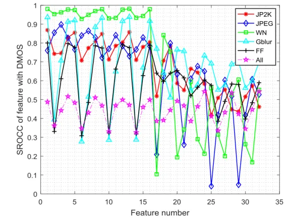
To validate our choice of features, we measured the correlation between each feature and the human differential mean opinion score (DMOS), by plotting the Spearman‘s rank ordered correlation coefficient (SROCC) values over the entire sets on the LIVE database II [28], as shown in Fig.4.
Fig. 4. SROCC for each of the features on the LIVE database
Note that no training procedure was involved here. From Fig.4, we can see the degree to which each feature correlates with human judgments and to which an image is affected by each distortion. For example, all the features correlate fairly well with the white noise distortion. The reason might be that the white noise increases the high-frequency content in the image and causes consequently the local changes in the relative order, based on which all the features are calculated. The ―variance‖ features correlate well with the Gaussian-blur distortion, may be due to the fact that the variance is related to the edges and textures in an image. The Gaussian blur can cause hazy textures or unclear edges, and then changes the variance correspondingly. The ―entropy‖ features captures relatively better for blur and FF (FF is a combination of JP2K and packet-loss errors) distortions. The reason may be that the Gaussian blur yields changes in image intensities, textures and edges; and these changes will be captured by the entropy that describes how much randomness (or uncertainty) there is in an image. Though there are several types of distortion involved in the compression distortion (e.g. quantization error, blocking effect, etc.), the general quality reduction can still be captured to some extent by the entropy alternations. The ―differential entropy‖ is the extension of
the entropy and could be negative (considering that the variables in the log directional derivative map could be negative), thus it becomes a complementary feature to the ―entropy‖. It should be noted that the performance of the single feature for different distortion types could not indicate if a feature is a good or bad indicator of an image. The complicate interactions between features also play an important role in the estimation of the image quality, though we have not yet deeply understood these interactions.
For clarity, we tabulated in Table 2 the performances of different features on LIVE database in terms of the SROCC. To save space, only the SROCCs of different features for JP2K distortion are listed. The results in Table 2 were obtained from 982 images on LIVE database without training.
Table 2
SROCC of different features for white noise
Feature ID f1 f2 f3 f4 f5 f6 f7 f8 f9 f10 f11 f12 f13 f14 f15 f16 SROCC 0.868 0.788 0.823 0.829 0.854 0.790 0.822 0.809 0.848 0.774 0.817 0.804 0.858 0.768 0.812 0.805 Feature ID f17 f18 f19 f20 f21 f22 f23 f24 f25 f26 f27 f28 f29 f30 f31 f32 SROCC 0.518 0.707 0.784 0.587 0.551 0.664 0.645 0.583 0.418 0.511 0.553 0.448 0.437 0.515 0.573 0.462
3.2. Evaluation of different regression methods
To select the regression method, we compared three regression methods: the SVR, the general regression neural network (GRNN) and the random forest (RF).
The SVR has been widely applied to image quality assessment problems [8], [13], since it could deal with high dimensional feature vectors [33]. Based on established statistical principles, the GRNN converges asymptotically with an increasing number of samples to the optimal regression surface [36].
Thus it is a powerful regression tool with a dynamic network structure [34]-[35]. It was shown in [36]-[37] that the GRNN could yield better results than the back-propagation network in terms of prediction performance. The Random Forest (RF) [38] was noted for its robustness against overfitting. The RF predicts new data by aggregating the predictions generated by all trees, and then takes the majority votes for classification and the average for regression.
The performances of these three regressors for the proposed features using 1000 train-test in LIVE database are tabulated in Table 3. Two correlation coefficients between the prediction results and the subjective scores were used: 1) the SROCC, which measures the prediction monotonicity; 2) the Pearson's (linear) correlation coefficient (LCC), which is related to the prediction linearity and can be considered as the measure of prediction accuracy. The LCC is ordinarily computed after passing the algorithmic scores through a logistic nonlinearity as described in [40]. A value of the SROCC/LCC closer to 1 indicates that the test metric predicts better the human opinions.
Table 3
Median SROCC and LCC across 1000 train-test in LIVE database using different regressors for proposed features
SROCC (Ratio of samples for training: 80%)
JP2K JPEG WN Gblur FF All
SVR 0.9483 0.9411 0.9564 0.9448 0.9172 0.9496
GRNN 0.9177 0.9354 0.9416 0.8909 0.9034 0.9278
RF 0.9421 0.9402 0.9555 0.9247 0.9175 0.9445
LCC (Ratio of samples for training: 80%)
JP2K JPEG WN Gblur FF All
SVR 0.9655 0.9674 0.9659 0.9426 0.9438 0.9560
GRNN 0.9446 0.9628 0.9537 0.9182 0.9344 0.9424
RF 0.9616 0.9679 0.9723 0.9539 0.9481 0.9592
We can see from the above table that the SVR and the RF outperform the GRNN. The SVR has a better prediction monotonicity than the RF; but the RF has a better prediction accuracy than the SVR. It is known that the RF is an effective tool in prediction [39], also confirmed by our experiments. But it is relatively complex and needs a long execution time. Since a NR metric is often used in the real-time assessment, we choose the SVR as our regression method.
3.3. Evaluation of the proposed IQA metric performance
To fairly evaluate the proposed IQA metric, we compared its performance to the representative FR IQA metric-structural similarity (SSIM) index and six state-of-the-art NR approaches (DIIVINE, BLIINDS-II, BRISQUE, CORNIA, GMLOG (M3) and FRIQUEE), by using the following well-known databases:
LIVE database II [28]: It consists of 29 reference images and their degraded versions with five types of distortion, i.e., JPEG 2000 compression (JP2K), JPEG compression (JPEG), additive white Gaussian noise (WN), Gaussian blurring (Gblur), and fast fading (FF). DMOSs associated with distorted images are provided.
The TID2008 database [41]: It contains 1700 test images derived from 25 reference images. There are 17 types of distortions for each reference image and four different scales for each distortion type.
CSIQ IQA database [42]: It consists of 30 reference images and their degraded versions with six different types of distortion at four to five different levels. DMOSs associated with distorted images are provided and in the range [0, 1], where a lower DMOS value indicates a higher quality.
LIVE In the Wild Image Quality Challenge Database [48]: It consists of over 350000 opinion scores on 1162 images of diverse authentic image distortions evaluated by over 8100 unique human observers.
For the TID 2008 database and the CSIQ database, we only tested images with four types of distortions that appear in LIVE database, i.e., JPEG, JP2K, WN, and Gblur.
Like the BRISQUE [13], in each train-test procedure, we also chose randomly 80% from the database as the train set and 20% as the test set so that no overlap between train and test content occurs. We repeated this random train-test procedure 1000 times and take the median performance over 1000 trials as the final overall performance.
A. Performance on LIVE database
Correlation with human judgements:
In Table 4,the FRIQUEE1 means that the FRIQUEE isdirectly used for testing, while FRIQUEE2 includes the train-test procedure. In Table 4,
we not only
show results on different distortion subsets in the LIVE database, but also the overall
performance (by performing train-test runs) on images with all
the
five types of distortion
in the database. The best one among the NR-IQA metrics is highlighted in boldface. To
show the generalization capability of the proposed approach, we also considered the case
when
a smaller part of the data-set is used for the training purpose
.
Table 4
Median SROCC and LCC across 1000 train-test combinations of LIVE database
SROCC
JP2K JPEG WN Gblur FF All
SSIM 0.9764 0.9594 0.9794 0.9661 0.9700 0.9487 DIIVINE 0.8465 0.8037 0.9768 0.9639 0.8392 0.8497 BLIINDS-II 0.9361 0.9004 0.9545 0.9161 0.8910 0.9223 BRISQUE 0.9349 0.9221 0.9560 0.9581 0.8891 0.9381 CORNIA 0.9383 0.9489 0.9730 0.9701 0.8911 0.9406 GMLOG 0.9196 0.9551 0.9800 0.9416 0.9113 0.9500 FRIQUEE1 0.8231 0.5735 0.9583 0.9071 0.8410 0.7470 FRIQUEE2 0.9373 0.9067 0.9783 0.9513 0.8754 0.9365 PROPOSED 0.9483 0.9411 0.9564 0.9448 0.9172 0.9496 LCC
JP2K JPEG WN Gblur FF All SSIM 0.9670 0.9573 0.9745 0.9040 0.9460 0.9383 DIIVINE 0.8416 0.7759 0.9562 0.9553 0.8401 0.8388 BLIINDS-II 0.9472 0.9286 0.9417 0.9101 0.9055 0.9226 BRISQUE 0.9375 0.9259 0.9630 0.9579 0.9118 0.9286 CORNIA 0.9483 0.9605 0.983 0.9677 0.9100 0.9417 GMLOG 0.9560 0.9836 0.9901 0.9604 0.9386 0.9510 FRIQUEE1 0.8297 0.6017 0.8961 0.9007 0.8491 0.7592 FRIQUEE2 0.9474 0.9383 0.9701 0.9496 0.8990 0.9425 PROPOSED 0.9655 0.9674 0.9659 0.9426 0.9438 0.9560
From Table 4, we can see that the proposed metric works well on each of the five distortions, especially on JP2K and FF. The reason may be that JP2K-compressed images manifest blur distortions and JP2K causes ringing effects (degradations around edges), while edges are reflected by the relative order based on which we constructed our IQA metric. It‘s the same for the FF distortion, since the FF is a combination of JP2K and packet-loss errors. As for the overall performance, our approach performed better than all the representative top performing NR-IQA algorithms, and the representative FR metric SSIM.
Statistical analyses: We performed the t-test [45] on the SROCC values obtained from the 1000 train-test trials in order to see if there is a statistically significant difference between each pair of tested metrics. The results in Table 5 were got by doing the one-side t-test where the confidence level is set to 95%. The standard deviation of them are around 0.02. In Table 5, ‗1‘ indicates that the row metric is statically superior to the column one; ‗−1‘ indicates that the row one is statistically worse than the column one; and ‗0‘ indicates that the row and column ones are statistically indistinguishable (or equivalent).
Table 5
Results of the two sample t-test performed between SROCC values obtained by different measures. 1(-1) indicates the algorithm in the row is statistically superior (inferior) than the algorithm in the column. 0 indicates the algorithm in the row is statistically equivalent to
the algorithm in the column
SSIM DIIVINE BLIINDS-II BRISQUE CORNIA GMLOG Proposed
SSIM 0 1 1 -1 -1 -1 -1 DIIVINE -1 0 -1 -1 -1 -1 -1 BLIINDS-II -1 1 0 -1 -1 -1 -1 BRISQUE 1 1 1 0 0 -1 -1 CORNIA 1 1 1 0 0 -1 -1 GMLOG 1 1 1 1 1 0 0 Proposed 1 1 1 1 1 0 0
From Table 5, we conclude that the SROCC value of the proposed one is statically higher than all other tested algorithms.
Linearity: The linearity of an IQA model makes it more convenient to benchmark an image processing algorithm such as image denoising. With a linear IQA model, the difference between the model‘s prediction scores is equivalent to the difference of human subjective scores. Therefore, a linear IQA model does not complicate the relationship between quality degradation and bit allocation [46].
For a uniform comparison of our proposed metric and other metrics (BRISQUE, BLIINDS-II, DIIVINE, SSIM), the 4-parameter logistic fitting was used to illustrate their linearity performance, as shown in Fig.5. Clearly, our method shows much better linearity than other ones.
(a) Proposed (b) BRISQUE (c) BLIINDS-II
(d) DIIVINE (f) SSIM
Fig.5. The scatter plots of the prediction results of proposed, BRISQUE, BLIINDS-II, DIIVINE, PSNR, SSIM versus the subjective score in LIVE database
To show the linearity more clearly, we also give the scatter plots of the proposed metric for each of the distortion types in LIVE database in Fig. 6.
(1) JP2K (2) JPEG (3) WN
(4) Gblur (5) FF
Fig.6. Scatter plots of the proposed metric. Predicted scores versus subjective DMOS on the distortion type: JP2K, JPEG, WN, Gblur and FF.
The objective of the distortion-specific experiment is to see how the algorithm will perform if we only have images with one particular type of distortion. Fig. 6 shows that our metric‘s performance has a nearly linear relationship with the DMOS and an almost uniform density along each axis.
B. Database Independence Experiment
Since a NR-IQA metric is based on learning, it is necessary to verify whether the parameters are over-fitted and the learned model is sensitive to different databases. To validate the independence of the proposed metric, following experiments are done: (1) training on LIVE and testing on CSIQ database; (2) training on CSIQ and testing on LIVE database; (3) training on LIVE and testing on TID2008 database ; (4) training on TID2008 and testing on LIVE database and (5) training on LIVE and testing on CSIQ+TID2008.
We trained and tested images with four types of distortions, including JPEG, JP2K, WN, and BLUR, presented in the TID2008 database, CSIQ database, and the LIVE database. We also report the performance of the model trained on LIVE and tested on CSIQ + TID2008 together in a common set. Note that the subjective scores provided in CSIQ and TID2008 databases are different: the former one is the DMOS (Difference Mean Opinion Score) within the range of [0, 1] and the latter is the MOS within the range of [0, 9]. To test CSIQ+TID2008 together in a common set, these two different scores should be mapped onto the same scale. Thus, in our experiments, we make the DMOS values in CSIQ unchanged and the MOS values in TID2008 be transformed into the
score
TID2008 defined as follow:2008
1
9
TID
scor
e
MO
S
(15)The results are listed in Table 6.
Table 6
Results of training and test in crossing databases
As is shown in Table 6, the proposed method performs well in terms of correlation with human opinions and its performance does not depend on the database.
Following the common practice, e.g. the BRISQUE, the results in Table 6 are got by testing the proposed model only on the distortions that it is trained for (including JP2K, JPEG, WN, Gblur). It remains then 384 images in TID2008 and 600 images in CSIQ, respectively. To investigate the performance of the proposed model on the discarded distortions, we also did the experiments as follows:
1) Trained on JP2K, JPEG, WN and Gblur in LIVE and tested on the different distortions in CSIQ (fnoise and contrast distortions): The SROCC is 0.295 and the LCC is 0.2861.
2) Trained on JP2K, JPEG, WN and Gblur in LIVE and tested on the different distortions in TID2008(the other 13 distortions):
The SROCC is 0.2636 and the LCC is 0.2529.
C. Performance on LIVE In the Wild Image Quality Challenge Database
The LIVE In the Wild Image Quality Challenge Database is the database that contains diverse authentic image distortions of a large number of images through a variety of modern mobile devices. In consideration
JP2K JPEG WN Gblur ALL
LIVE for training and CSIQ for test
SROCC 0.8777 0.9140 0.9113 0.9250 0.9136
LCC 0.9056 0.9511 0.9121 0.9406 0.9320
CSIQ for training and LIVE for test
SROCC 0.9179 0.9624 0.9783 0.8742 0.9364
LCC 0.9140 0.9647 0.9321 0.8526 0.9232
LIVE for training and TID2008 for test
SROCC 0.9233 0.9398 0.8479 0.8807 0.9173
LCC 0.9094 0.9521 0.8412 0.8720 0.9029
TID2008 for training and LIVE for test
SROCC 0.9331 0.9596 0.9763 0.9029 0.9302
LCC 0.8900 0.9622 0.9723 0.8827 0.8924
LIVE for training and CSIQ+TID2008 for test
SROCC 0.8673 0.9010 0.8651 0.8690 0.8911
of its huge difference with the prior traditional databases and for a fair comparison to some extent, Table 7 shows the representative NR IQA models‘ performances obtained by being trained on the LIVE In the Wild Image Quality Challenge Database and tested on the same database. The listed models are all learnt using
the SVR. Furthermore, the FRIQUEE that is especially designed for this database is also listed. The median of 100 train-test procedures are reported as the result. Not surprisingly, the FRIQUEE performs the best on this database among all the representative models. It is noted that the BRSIQUE, the GMLOG and the proposed one perform similarly. This further demonstrates the robustness of the proposed model.
Table 7
Results on LIVE In the Wild Image Quality Challenge Database by training and testing on the same database
IQA model SROCC LCC BRISQUE 0.6131 0.6456
GMLOG 0.5945 0.6173
FRIQUEE 0.7238 0.7146 Proposed 0.5995 0.6259
3.4. Evaluation of the implementation complexity
In this subsection, we compare the complexity of the proposed metric with that of other algorithms. To ensure a fair comparison, we use un-optimized MATLAB codes for all of these algorithms. In Table 8 we list the amount of time (in seconds) to compute each quality measure on a gray scale image with the resolution 768×512 on a 2.66 GHz Intel Core2 Quad CPU with 4 GB of RAM.
Table 8
Average execution time for different metrics (seconds)
Algorithm DIIVINE BLIINDS-II BRISQUE FRIQUEE GMLOG CORNIA Proposed
Time 52.94 136.05 0.44 119.93 0.310 8.211 0.69
As shown in Table 8, the DIIVINE, the BLIINDS-II, the CORNIA and the FRIQUEE require much more time than the proposed method, the BRISQUE and the GMLOG. That is mainly because that the
DIIVINE needs to extract too many features (88 features) in the wavelet domain and the BLIINDS-II is based on block-wise DCT coefficients computations and pooling. The FRIQUEE, however, extracted a
huge number of features (560 features) for an image. From Table 8, we can see that the proposed model is almost 173 times faster than the FRIQUEE and just a little slower than the BRISQUE and the GMLOG.
3.5. Discussion
Our experimental results showed that the proposed method is effective and efficient. The success of the proposed metric can be related to its following aspects: (1) the degree of warping caused by different types of image distortions manifests itself multifariously, which is effectively illustrated by the variation of the marginal distribution of the relative order coefficients; (2) the generalized Laplace model fits better the empirical statistics of the log histogram of log directional derivatives.
We have presented a simple but effective general-purpose NR-IQA metric that evaluates image quality without any reference image or any assumption on the distortion type. The proposed method uses 32 features, obtained from the log histograms of log horizontal, vertical, main-diagonal and secondary-diagonal derivatives, along with kurtosis, variance, differential entropy and entropy. To capture the multiscale behavior of images, all those features are then computed at two scales. The metric uses the SVR to map the feature vector to a quality score. Our experimental results showed that the proposed metric has a better performance than the representative NR IQA metrics on the tested databases. It is also consistent and stable across four benchmark databases. In addition, its simplicity makes it a good candidate of real-time blind assessment of visual quality.
A big limitation of the proposed method is ―opinion-aware‖ (OA). It needs to be trained on a database of human rated distorted images with their associated subjective opinion scores. The performance of the metric depends on the comprehensiveness of the database. If the metric is applied on a new distortion non-existent in the database, we have no idea about its possible performance. Considering that it is too expensive and time-consuming to establish a database that cover all existing distortions, not to speak of new types of distortion brought by new technologies in the future, we would like to extent our method to an ―opinion-unware‖ (OU) or even an OU and ―distortion-unware‖ (DU) NR-IQA metric in the future. For example, the OU-DU IQA model called Natural Image Quality Evaluator (NIQE) [47] used similar NSS features to those used in the BRISQUE. Our experiment results showed that our metric outperformed the BRISQUE. This suggests that our relative order-based features may have the potential to be better ―perceptual quality aware‖ features that could be used in a new OU-DU NR-IQA metric. In addition, a relevant research [52] also shows how to use the NSS features for biomedical images.
Acknowledgements
The authors are grateful to anonymous reviewers for insightful and helpful comments about the manuscript.
This work was supported partly by the Natural Science Foundation of China under Grant 61762004, Science and Technology Project Founded by the Education Department of Jiangxi Province (GJJ170455) and the Open Fund Project of Jiangxi Engineering Laboratory on Radioactive Geoscience and Big Data Technology under Grant JELRGBDT201702. This work was also supported in part by the Ph.D. Research Startup Foundation of East China University of Technology under Grants DHBK2016119 and DHBK2016120.
References
[1] Z. Wang, A. C. Bovik, H. R. Sheikh, and E. P. Simoncelli, Image quality assessment: from error visibility to structural similarity, IEEE Transaction on Image Processing 13 ( 4) (2004) 600–612.
[2] X. Zhang, X. Feng, W, Wang, and W. Xue, Edge strength similarity for image quality assessment, IEEE Signal Processing Letters 20 (4) (2013) 319-322.
[3] Z. M. P. Sazzad, Y. Kawayoke, and Y, Horita. No-reference image quality assessment for JPEG2000 based on spatial features, Signal Processing: Image Communication 23 (4) (2008) 257-268.
[4] S. Suthaharan, No-reference visually significant blocking artifact metric for natural scene images, Signal Processing 89(8) (2009) 1647–1652.
[5] X. Zhu and P. Milanfar, A no-reference sharpness metric sensitive to blur and noise, IEEE International Conference on Multimedia and Expo, San Diego, CA,(2009) 64-69.
[6] M. A. Saad, A. C. Bovik, and L. Cormack, A DCT statistics-based blind image quality index, IEEE Signal Processing Letters 17(6) (2010) 583-586.
[7] A. K. Moorthy and A. C. Bovik, A two-step framework for constructing blind image quality Indices, IEEE Signal Processing Letters 17(5) (2010) 513-516.
[8] A. K. Moorthy and A. C. Bovik, Blind image quality assessment: from natural scene statistics to perceptual quality, IEEE Transactions on Image Processing 20 (12) (2011) 3350-3364.
[9] H. Tang, N. Joshi, and A. Kapoor, Learning a blind measure of perceptual image quality, IEEE Conference on Computer Vision and Pattern Recognition (2011) 305-312.
[10] C. Li, A. C. Bovik, and X. Wu, Blind image quality assessment using a general regression neural network, IEEE Transactions on. Neural Network 22 (5) (2011) 793-799.
[11] P. Ye and D. Doermann, No-reference image quality assessment using visual codebooks, IEEE Transactions on Image Processing 21 (7) (2012) 3129-3137.
[12] M. A. Saad, A. C. Bovik, and C. Carrier, Blind Image Quality Assessment: a natural scene statistics approach in the DCT domain, IEEE Transactions on Image Processing 21(8) (2012) 3339–3352.
[13] A. Mittal, A. K. Moorthy, and A. C. Bovik, No-reference image quality assessment in the spatial domain, IEEE Transactions on Image Processing 21( 12) (2012) 4695-4708.
[14] P. Ye, J. Kumar, L. Kang, D. S. Doermann: Unsupervised feature learning framework for no-reference image quality assessment. CVPR 2012: 1098-1105.
[15] L. X. Liu, B. Liu, H. Huang and A. C. Bovik, ―No-reference image quality assessment based on spatial and spectral entropies,‖ Signal Processing: Image Communication, vol. 29, no. 8, pp. 856-863, 2014.
[16] W. F. Xue, L. Zhang and X. Q. Mou, ―Learning without human scores for blind image quality assessment,‖ in Proc. of IEEE Conference on Computer Vision and Pattern Recognition (CVPR), pp. 995-1002, June 23-28, 2013.
[17] Q. Li, W. Lin, J. Xu, Y. Fang: Blind Image Quality Assessment Using Statistical Structural and Luminance Features. IEEE Trans. Multimedia 18(12): 2457-2469 (2016).
[18] L. Li, W. Lin, X. Wang, G. Yang, K. Bahrami, A. C. Kot: No-Reference Image Blur Assessment Based on Discrete Orthogonal Moments. IEEE Trans. Cybernetics 46(1): 39-50 (2016).
[19] K. Gu, G. Zhai, W. Lin, X. Yang, W. Zhang: No-Reference Image Sharpness Assessment in Autoregressive Parameter Space. IEEE Trans. Image Processing 24(10): 3218-3231 (2015).
[20] W Xue, X Mou, L Zhang, AC Bovik, Blind image quality assessment using joint statistics of gradient magnitude and Laplacian features, IEEE Transactions on Image Processing, 2014.
[21] D. Ghadiyaram and A.C. Bovik, ―Perceptual quality prediction on authentically distorted images using a bag of features approach,‖ Journal of Vision, January 2017.
[22] J. Huang, Mumford D, Statistics of natural images and models, IEEE Conference on Computer Vision and Pattern Recognition (1999) 541–547.
[23] G. Cheng, J. Huang, Z. Liu, L. Cheng, Image quality assessment using natural image statistics in gradient domain, International Journal of Electronics and Communications (AEÜ) 65(2011) 392–397.
[24] A. Liu, W. Lin, M. Narwaria, Image quality assessment based on gradient similarity, IEEE Transactions on Image Processing 21( 4) (2012) 1500-1512.
[25] G. Chen, C. Yang, and S. Xie, ―Gradient-based structural similarity for image quality assessment,‖ in Proc. Int. Conf. Image Process., 2006,pp. 2929–2932.
[26] A. Srivastava, A. B. Lee, E. P. Simoncelli, and S. Zhu, On advances in statistical modeling of natural images, Journal of Mathematical Imaging and Vision 18 (1) (2003) 17–33.
[27] T.M. Cover and J.A. Thomas, Elements of Information Theory, John Wiley & Sons, Inc., 1985
[28] H.R. Sheikh, Z. Wang, L. Cormack, and A.C. Bovik, LIVE image quality assessment database release 2.<http://live.ece.utexas.edu/ research/ quality>.
[29] B. Schölkopf, A. J. Smola, R. C. Williamson, and P. L. Bartlett, New support vector algorithms, Neural Computation 12(5) (2000) 1207–1245.
[30] C. Chang and C. Lin. (2001). LIBSVM: A Library for Support Vector Machines [Online]. Available: http://www.csie.ntu.edu.tw/∼cjlin/libsvm/
[31] M. Narwaria and W. Lin, Objective image quality assessment based on support vector regression, IEEE Transactions on Neural Network, 21(3) (2010) 515–519.
[32] M. Narwaria and W. Lin, SVD-based quality metric for image and video using machine learning, IEEE Transactions on Systems, Man, and Cybernetics, Part B: Cybernetics, 42(2)(2012) 347–364.
[33] C. J. C. Burges, A tutorial on support vector machines for pattern recognition, Data Mining and Knowledge Discovery, 2(2) (1998)121–167.
[34] D. F. Specht, A general regression neural network,IEEE Transactions on Neural Network 2 (6) (1991) 568–576.
[35] S. Chartier, M. Boukadoum, and M. Amiri, BAM learning of nonlinearly separable tasks by using an asymmetrical output function and reinforcement learning,‖ IEEE Transactions on Neural Network 20(8) (2009) 1281–1292.
[36] D. Tomandl and A. Schober, A modified general regression neural network (MGRNN) with new, efficient training algorithms as a robust‗black box‘-tool for data analysis, Neural Network 14(8) (2001) 1023–1034.
[37] Q. Li, Q. Meng, J. Cai, H. Yoshino, and A. Mochida, Predicting hourly cooling load in the building: A comparison of support vector machine and different artificial neural networks, Energy Conversion and Management 50(1) (2009) 90–96.
[38] L. Breiman, Random forests, Machine Learning 45(1) (2001) 5–32.
[39] Z.Gu, L. Zhang, X. Liu, and H. Li, Learning quality-aware filters for no-reference image quality assessment, IEEE International Conference on Multimedia and Expo, (2014) 1-6.
[40] H. R. Sheikh, M. F. Sabir, and A. C. Bovik, A statistical evaluation of recent full reference image quality assessment algorithms, IEEE Transactions on Image Processing 15(11) (2006) 3440–3451.
[41] N. Ponomarenko, V. Lukin, A. Zelensky, K. Egiazarian, M. Carli, and F. Battisti, TID2008—A database for evaluation of full-reference visual quality assessment metrics, Advances of Modern Radioelectronics 10 (4) (2009) 30–45.
[42] E. C. Larson and D. M. Chandler. Most apparent distortion: Full-reference image quality assessment and the role of strategy, Journal of Electronic Imaging 19 (1) (2010) 1-21.
[43] Y. Horita, K. Shibata, Y. Kawayoke, et al., MICT image quality evaluation database [Online]. Available: <http://mict.eng.u-toyama.ac.jp/mictdb.html.2000>.
[44] A. Ninassi, P.L. Calet, F. Autrusseau, Pseudo no reference image quality metric using perceptual data hiding, SPIE Human Vision and Electronic Imaging 6057(08) (2006)146-157.
[45] D. Sheskin, Handbook of Parametric and Nonparametric Statistical Procedures. London, U.K.: Chapman & Hall, 2004 [46] W. Xue, L. Zhang, X. Mou, and A. C. Bovik. Gradient magnitude similarity deviation: A highly efficient perceptual image
quality index, IEEE Transactions on Image Processing 23(2) (2014) 684–695.
[47] A. Mittal, R. Soundararajan and A. C. Bovik, Making a Completely Blind Image Quality Analyzer, IEEE Signal Processing Letters 22(3) (2013) 209-212.
[48] D. Ghadiyaram and A.C. Bovik, ―Massive online crowdsourced study of subjective and objective picture quality,‖ IEEE Transactions on Image Processing, January 2016.
[49] T. Wang, H. Shu, H.Jia, B. Li, L. Zhang. Blind image quality assessment using natural scene statistics in the gradient domain, Asia Modelling Symposium, 2014:56-60.
[50] H. Jia, Q. Sun, Z. Ji, T. Wang, Q. Wang. No-reference image quality assessment based on natural scene statistics and gradient magnitude similarity,Optical Engineering 53(11), 113110.
[51] Y. Gong, I.F. Sbalzarini, Image enhancement by gradient distribution specification, in: Computer Vision—ACCV 2014 Workshops, Springer, 2014, pp. 47-62.
[52] Y. Gong, I.F. Sbalzarini, A natural-scene gradient distribution prior and its application in light-microscopy image processing, IEEE J. Sel. Top. Signal Process. 10 (1) (2016) 99–114.