HAL Id: hal-01848201
https://hal-mines-albi.archives-ouvertes.fr/hal-01848201
Submitted on 24 Jul 2018
HAL is a multi-disciplinary open access
archive for the deposit and dissemination of
sci-entific research documents, whether they are
pub-lished or not. The documents may come from
teaching and research institutions in France or
abroad, or from public or private research centers.
L’archive ouverte pluridisciplinaire HAL, est
destinée au dépôt et à la diffusion de documents
scientifiques de niveau recherche, publiés ou non,
émanant des établissements d’enseignement et de
recherche français ou étrangers, des laboratoires
publics ou privés.
A combined DEM & FEM approach for modelling roll
compaction process
Alon Mazor, Luca Orefice, Abderrahim Michrafy, Alain de Ryck, Johannes
Khinast
To cite this version:
Alon Mazor, Luca Orefice, Abderrahim Michrafy, Alain de Ryck, Johannes Khinast. A combined
DEM & FEM approach for modelling roll compaction process. Powder Technology, Elsevier, 2018,
337, pp.3-16. �10.1016/j.powtec.2017.04.053�. �hal-01848201�
A combined DEM & FEM approach for modelling roll compaction process
Alon Mazor
a,1, Luca Orefice
b,1, Abderrahim Michrafy
a,*
, Alain de Ryck
a, Johannes G. Khinast
b,c,*
aUniversité de Toulouse, Mines Albi, CNRS, Centre RAPSODEE, Albi, FrancebResearch Center Pharmaceutical Engineering GmbH, Graz, Austria
cGraz University of Technology, Institute of Process and Particle Engineering, 8010 Graz, Austria
Keywords: Roll compaction FEM DEM Coarse graining Density distribution
A B S T R A C T
Roll compaction is a continuous manufacturing process aiming to produce particulate granules from pow-ders. A roll press typically consists of a screw feeding system, two rolls and a side sealing. Despite its conceptual simplicity, numerical modelling of the process is challenging due to the complexity involving two different mechanisms: feeding by the screw and powder compaction between the rolls.
To represent the materials’ behaviour both in the feeding zone and in the compaction area, a combined three-dimensional Discrete Elements Method (DEM) and Finite Elements Method (FEM) is developed in this work. The DEM, which is a more suitable method to describe the flow of granular material, is used to model the motion of particles in the feeding zone. As the granular material deforms under high pressure between rolls, FEM offers a more versatile approach to represent the powder behaviour and frictional conditions. In the proposed approach the DEM and FEM are treated as complementary methods, enabling us to take advantages of the strengths of both.
In this proposed approach, the time dependent velocity field of the particles at the end of the screw feeder is evaluated as a continuous field using the coarse graining (CG) framework, which was used as input data for the FEM model. FEM is then used to simulate the powder compaction in between the rolls, and the resultant roll pressure and ribbon relative density are obtained.
Our results show a direct correlation between the particle velocity driven by the screw conveyor and the roll pressure, both oscillating with the same period. This translates into an anisotropic ribbon with a density profile varying sinusoidally along its width, with a period equal to the duration of a screw turn.
1. Introduction
Roll compaction is a process designed to compact fine powders to produce particulate granules, and it pertains to continuous man-ufacturing procedures. During the process, powder is subjected to high pressure from the rolls, leading to the formation of compacted ribbons, which are later milled into granules. The ribbon’s rela-tive density largely influences the compactibility of granules and subsequently the final solid dosage form (i.e., compacted tablets) properties. Therefore, relative density is commonly used as a critical quality parameter of the roll compaction process. In order to ensure the consistency, repeatability and quality of the final dosage form, it is important to avoid heterogeneity of the produced ribbon.
*Corresponding authors.
E-mail addresses:[email protected](A. Michrafy),[email protected] (J.G. Khinast).
1 First authorship equally shared.
A typical roll compactor consists of a single rotating screw, which feeds the material into a gap between two counter-rotating rolls and cheek plates on the sides to avoid leakage. The conveying of pow-der towards the rolls have a large influence on the roll compaction process. Experimental work showed that the delivery of powder by a screw feed is linearly related to the screw speed[1,2]. An appropri-ate compaction is reached and maintained with a screw to roll speed ratio laying in a specific range. Simon and Guigon[2]also showed that by using a single feed screw, the compacted ribbon was nei-ther homogeneous along the ribbon’s width nor in time. Moreover, these fluctuations have the same period of the screw rotation. The impact of the screw motion on the compaction process is relevant for the ribbon properties, albeit not in a trivial way. Not only does the screw design affect particle flow[3]and mixing[4], but also powder properties play an important role[1,5,6]. In addition, the behaviour of simple screw feeders will differ as soon as they are coupled with other devices, which will alter the flow properties and the pressure distributions inside. A numerical example can be found in[7].
Numerous studies investigated analytically the roll compaction process. The most well-known analytical model is the Johanson
model[8], which is able to determine the pressure along the roll surface, torque and separating force of the rolls, based on the phys-ical characteristics of the powder and dimensions of the press. The main limitation of the classical Johanson model is that it does not include the important process parameters of roll and screw speeds, which led to the extension of this model by Reynolds et al.[9]. How-ever, these models are only one-dimensional and do not take into account the non-uniformity of the conveying of powder and as a result the non uniform roll pressure and ribbon’s density distribu-tion. Bi et al.[10]attempted to overcome this limitation by extending Johanson’s model to account for a non-uniform powder velocity in the nip region. However, their result is of little experimental use because the model developed introduces a high variability in the pre-dicted pressure peak, and because the estimation of a key parameter of the model cannot be measured experimentally.
To resolve this, Finite Elements Method (FEM) modelling was adopted to simulate the roll compaction process, starting with plane strain two-dimensional cases[11–14], followed by the development of three-dimensional models to provide greater insight into the pressure and density distribution during the roll compaction pro-cesses [15–18]. In these models, the effect of the screw feeder is approximately represented by a uniform or oscillatory inlet feed-ing pressure at the entry angle. Liu and Wassgren[19]implemented a mass-corrected version of Johanson’s model analogous to[10]in a two-dimensional FEM model, yet based on two experimentally-determined fitting parameters. The results show a better agreement with the experimental pressure profile when compared to the origi-nal Johanson’s model. However, the model still relies on experimen-tal data, and only uses an arbitrary constant feed pressure, which does not account for the complex pressure pattern created by the screw conveyor. Michrafy et al.[17]investigated the effect of a con-stant inlet feeding velocity on the roll compaction process using cheek plates, which resulted in higher pressure and relative den-sity in the middle of the ribbon compared to the edges. Cunningham et al.[18]compared a uniform inlet feeding velocity to a linearly decreasing velocity from the centre to the edges, where both cases have no friction between powder and cheek plates. In the case of uni-form inlet feeding velocity, the maximum roll pressure and relative density were the same along the ribbon’s width. Using a non-uniform inlet feeding velocity, the powder is fed rather in the middle than at the edges, and consequently results in higher maximum roll pres-sure, shear stresses and relative density in the middle of the ribbon. These results are comparable with experiments only with the under-standing that the conveying of powder in between rolls have a direct effect of the process. In conclusion, in all of the previous FEM mod-els of roll compaction the inlet velocity or feed pressure values are chosen arbitrarily and do not represent the effect of screw feed-ing. Therefore, features associated to the periodic feeding, such as a non-uniform conveying in both space and time, are still unaccounted for.
The numerical modelling of the roll compaction process remains challenging due to the complexity involving two different mecha-nisms: the feeding by the screw conveyor and the powder com-paction between the rolls. On one side, the incoming particle flow is a key parameter strongly influencing the compaction process, since it dictates the pace of the process and affects the homogeneity of the compacted ribbon. On the other hand, the material deformation under high stress, and the frictional conditions in the compaction region, are the fundamental quantities needed to model the system. In order to address these issues, we developed a combined three-dimensional Discrete Elements Method (DEM) and FEM methodology. DEM is naturally suited to model the conveying pro-cess and will be used to study the particle flow in the feeding zone. The results will be used as boundary inlet conditions for the FEM modelling of the compaction process, which is the best approach to study the compaction of porous materials under high pressure. In
our work, the DEM and FEM are treated as complementary methods: combining them in the study of roll compaction enables us to take advantage of their strengths in the regions where they are respec-tively best suited. The aim of our study is therefore to improve the existing numerical models, leading to a more realistic description of the process which will head us to a better prediction of the final ribbon quality.
2. Materials and methods
2.1. Roll compaction design and process parameters
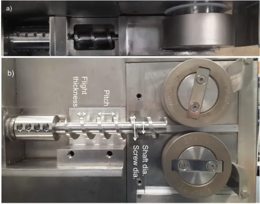
This work is based on the Komarek B050H Laboratory Press (K.R. Komarek Inc., Wood Dale, IL, USA). The Komarek roll compactor is constructed with a horizontal screw conveyor and two counter-rotating rolls with fixed side seals (i.e. cheek plates) in between (see Fig. 1). The process parameters of minimum gap width between rolls, rolls speed and screw speed were set to dmin= 0
.
2 cm, yR= 6 rpmand yS = 48 rpm, respectively. Further details about the roll press
dimensions can be found inTable 1.
2.2. Powder
The powder used in this work is microcrystalline cellulose (MCC) (Avicel PH 101, FMC BioPolymer, Philadelphia, PA, USA). MCC is one of the most important and widely employed excipients in the pharmaceutical industry. It has excellent compressibility proper-ties and is used as diluent for drug formulations in the tableting process[20,21]. The true density of the powder blend was deter-mined using a helium pycnometer (Accupyc 1330, Micromeritics Instrument Corp., Norcross, GA, USA) as qtrue = 1.56 g
/
cm3.2.3. Discrete Elements Method
The Discrete Elements Method [22]is a numerical method for computing the dynamics of a large ensemble of small compo-nents, typically spherical particles. Particles interact with each other according to a special interaction law and can be influenced by external force fields, such as gravity. In addition, they interact with geometrical objects, which are generally located inside the simula-tion domain (e.g., walls or pipes) and may affect their movement. The interaction law governing the forces experienced by objects upon collision commonly accounts for an elastic repulsive term (due to the rigidity of the bodies) and a dissipative term (due to friction). In a DEM simulation, contacts between the objects at each time step and forces generated by the collisions are computed. Next, the dynam-ics of the components are evaluated and the equations of motion are integrated, with the position and velocity of objects being updated accordingly. This is repeated at each time step for the entire duration of the simulation.
Discrete Element modelling is suitable for studying the flow of solid particulate materials since the detailed dynamics of every sin-gle particle are determined at any moment and the physics of the macroscopic medium is based on it. However, the results greatly depend on the interaction laws between the objects. For instance, accounting for the particle deformation or breakage caused by high pressure is difficult as is the modelling of a (realistically) large ensemble of particles due to very high computational cost. As such, although the DEM model in this study is unsuitable for modelling the compaction process, it can be employed to model the particle flow transported by the screw conveyor inside the compaction region.
2.3.1. Contact model and parameters
In DEM simulations, objects interact according to the well-known Hertzian spring-dashpot contact model [23,24]. We used rigid, frictional, non-deformable spheres of uniformly distributed
Fig. 1. Komarek B050H roll compactor; a) top view and b) side view (w/o feed barrel and side seals).
poly-disperse radius in the range rP± 10% to model the powder
par-ticles and for the compactor components we employed frictional, non-deformable stereolithographical (STL) meshes. The mean parti-cle radius was chosen such that every partiparti-cle could fit through the gap of 0.2 cm between the screw blade and the conveyor casing (see Table 1), with the polydispersity eliminating crystallisation effects between particles that may affect the flow[25,26]. A common prac-tice in DEM is to use mesoscopic particles in the simulations, i.e., much bigger than the ones in the experiment. We observed that the particle size is not affecting the velocity profile of the particles inside of the screw, and therefore the size chosen is the biggest possible one fitting through the screw clearance (the distance between the screw blade and the casing) to reduce the computational expense. However, we monitored the forces acting on the particles and their overlap to guarantee that no jamming occurred. The interactions account for sliding and rolling friction. In our model, the particles were composed of micro-crystalline cellulose(MCC) and the com-pactor’s components material was steel, material properties taken from[27–31]. We recorded the DEM simulation data every 2 × 10³
time steps of length dt, resulting in a time interval of duration Dt between the monitored snapshots. The simulation parameters and
Table 1
Komarek B050H roll compactor dimensions.
Part Symbol Size [cm]
Screw feeder Screw length ls 15 Pitch length lp 1.95 Flight thickness tsf 0.5 Flight diameter dsf 3.5 Shaft diameter dss 1.9 Casing diameter dc 3.8 Roll press Rolls diameter dR 10 Rolls width wR 3.8
Minimum gap width dmin 0.2
the material properties are reported inTable 2. The simulations used for this study were performed using the open source DEM particle simulation code LIGGGHTS ®[32].
2.3.2. Discrete Element model
A schematic representation of the DEM model of the compactor is shown inFig. 2, all the geometry parameters being listed inTable 1. Each simulation is composed of 3 distinct phases: loading, transient and steady flow.
During the loading phase, the system is filled with particles. To this end, 7500 particles were loaded into a parallelepipedal volume inside the hopper (A) every second of physical time. As soon as they reached the bottom, the screw (B) dragged them towards the com-paction region (D) that gradually began to fill. The screw velocity during this phase was a fraction of the one used at full speed dur-ing the compaction process, and the rolls speed was set to zero. A wall prevented the particles from exiting the compaction region
Table 2
Parameters used in the DEM simulations.
Parameters and material properties Symbol Value Particle mass density [g/cm3] q
P 1.56
Particle mean radius [cm] rP 0.09
Particle Young’s modulus [Pa] YP 1.0 × 10¹⁰
Conveyor Young’s modulus [Pa] YC 1.8 × 10¹¹
Particle Poisson ratio [–] mP 0.30
Conveyor Poisson ratio [–] mC 0.30
Particle-particle restitution coeff. [–] ePP 0.83
Particle-conveyor restitution coeff. [–] ePC 0.80
Particle-particle sliding friction coeff. [–] lPPsliding 0.53
Particle-conveyor sliding friction coeff. [–] lPCsliding 0.20
Particle-particle rolling friction coeff. [–] lPProlling 0.25 Particle-conveyor rolling friction coeff. [–] lPCrolling 0.10
Screw operational velocity [rpm] yS 48
Rolls operational velocity [rpm] yR 6
Gap width [cm] d 0.36 Time step [s] dt 5.0 × 10⁻⁶
Fig. 2. Schematics of the RC implemented in the DEM model. A: hopper. B: screw
conveyor. C: compaction region inlet (transition area from DEM to FEM modelling). D: compaction region. E: counter-rotating compaction rolls (the rotation direction is indicated by the arrows).
through the inter-rollers gap. The loading phase continued until both the compaction region and the hopper were completely filled with particles.
Once the desired fill level was achieved, the transient phase began and the wall blocking the exit through the gap between the rolls (E) was removed. Both the screw and roll velocities were set to their operational values of ySand yRrespectively, and the particles began
to flow through the gap. The particle loading in the hopper remained unchanged in order to keep it constantly full and to preserve the overall number of particles in the system at around 8 × 10⁴. The
pur-pose of this phase is a transition from the static loading phase to the steady state phase.
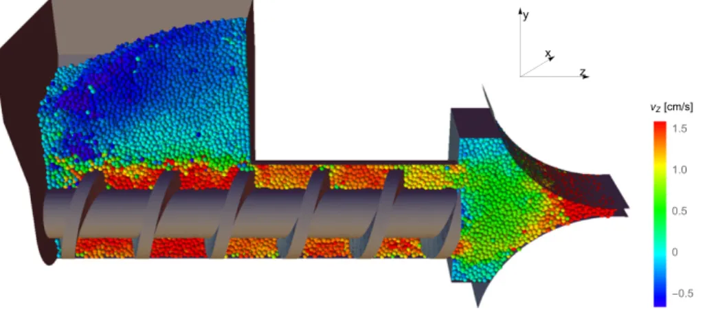
The steady-state regime is reached when there are negligible fluc-tuations both in the mean volumetric flow and in the mean axial velocity of the particles measured along certain planes normal to the axis. A snapshot of the steady-state system is illustrated inFig. 3. As it can be seen, the axial velocity of the particles, which is almost uni-form inside the screw barrel, quickly drops as soon as they approach the compaction region inlet, where they experience a considerable back-pressure due to a high density in this area. Regions of low veloc-ity are located against the back wall of the compaction chamber. The particles’ velocity rises as they approach the gap, where they are compacted (in reality) and are expelled. In this flowing regime, the data of interest were recorded along the inlet plane (C) between
the screw conveyor and the compaction region and averaged, as explained below.
The purpose of the DEM model is to simulate the particle flow at the inlet of the compaction region, and not other quantities of central importance for the compaction process, such as the pressure. This is due to the fact that the interaction laws are not suitable for the mod-elling of this aspect. Moreover, FEM is the natural tool to approach a study of the pressure distribution. For this reason, to avoid too high particle overlap in the neighbourhood of the screw tip, and conse-quent unphysical behaviour of the particle dynamics, the gap size in DEM is much bigger than the respective FEM and experimental coun-terparts. A bigger gap allows the particles to easily flow out from the compaction chamber, preventing them from overlapping under the pressure exerted by the screw rotation. In addition, the gap has to be small enough to avoid the compaction chamber to empty which would lead to an inhomogeneous packing of the inflowing particles. Similar constricted outflow conditions have been already used in the literature, e.g., in[7].
Because of this artefact the particles in the inflow region are densely packed but still in a free-flow condition, granting the appli-cability of the Hertz-Mindlin interaction law. As a consequence, the powder density at the inlet corresponds to tapped MCC, which justifies the FEM inlet density assumption. Lastly, since both the geometry of the inlet and the density of the powder are the same in both DEM and FEM, and the velocity field, by definition, coincides, both volumetric and mass throughputs at the inlet of the different models match.
2.4. Finite Elements Method (FEM)
In this work, FEM is used to investigate the effect of screw feeding velocity on the roll compaction process by obtaining the magnitudes and directions of stresses and strains. The FEM model was solved as a steady-sate problem using the Arbitrary Lagrangian-Eulerian (ALE) adaptive meshing in Abaqus/Explicit v6.14. The ALE adaptive mesh domain for steady-state problems is used to model material flow-ing through the mesh, and consist of two Eulerian boundary regions (inflow and outflow), connected by a Lagrangian or Sliding boundary region[33].
2.4.1. FEM model
The FEM model is based on the geometry of the desired roll com-pactor. In the case of the Komarek press, the rolls’ diameter and width are dR = 10 cm and wR = 3
.
8 cm respectively, and definedas analytic rigid surfaces. The minimum gap width between the rolls remains fixed during FEM modelling, having a value of dmin=
0
.
2 cm. Once sketching the press dimensions, the region between theFig. 3. Vertical section of one snapshot of the system at steady-state, the particles are coloured according to their axial velocity vz. (For interpretation of the references to colour
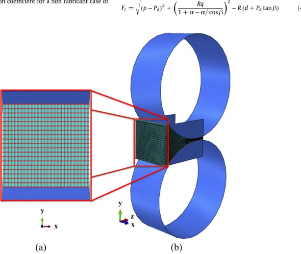
rolls is discretised and meshed by 80,000 C3D8R three-dimensional continuum reduced integration elements. The FEM model of the roll compactor can be visualized inFig. 4. It is important to men-tion that due to the non symmetric feeding velocity, the model was constructed fully without taking into account symmetry conditions, which are usually applied to reduce computational costs.
2.4.2. Boundary conditions
In FEM, introducing the powder into the roll compaction sys-tem is possible by two different boundary conditions: either pres-sure or velocity inlet. Applying a non-uniform prespres-sure on each element face in an ALE adaptive mesh domain causes a separate Lagrangian boundary region. Since Lagrangian corners are formed where Lagrangian edges meet, all nodes will follow the material in every direction, and each region becomes nonadaptive[33]. On the other hand, by assigning a non-uniform nodal velocity boundary con-dition to the inlet Eulerian region (Fig. 4), there is no alteration of the nodes to be nonadaptive and therefore was the approach cho-sen for this work. The inlet material density was set to be the tapped powder density as a result of the screw feeding. The MCC Avicel PH 101 tapped density qtappedis about 0.47 g
/
cm3, which correspondsto an initial relative density qrelof 0.3. In addition, the rolls rotational boundary condition of ±0
.
63 rad/s about the x-axis was defined to represent yR.As mentioned previously, the ALE method enables working both with the advantages of Lagrangian and Eulerian elements in the same part[34]. While the inlet and outlet surfaces are defined as Eulerian regions, the surfaces that are in contact with the rolls are defined as sliding surfaces. The contact between the powder mesh and the outer surfaces representing the sealing and rolls is defined as surface-to-surface with Coulomb friction coefficient for a non lubricant case of
l = 0
.
4[13,15,16].2.4.3. Constitutive model for continuum modelling
In our FEM modelling, the behaviour of the powder, considered as a continuous, porous, compressible material, is described using the density-dependent Drucker-Prager Cap (DPC) model [35,36] and implemented by an external user-defined VUSDFLD Fortran subroutine.
Assuming the material is isotropic, the model consists of three different parts: a shear failure surface Fsrepresenting shearing flow,
a cap surface Fcrepresenting an inelastic hardening for plastic
com-paction and a transition zone Ftbetween the two surfaces, providing
smooth surface to avoid singularities in the modelling. The shear fail-ure is simply described by a straight line on the p-q plane and defined as:
Fs= q − d − p tan b = 0 (1)
The slope of the line represents the friction angle b, and the intersection with the q axis represents the cohesion, d. Here p rep-resents the hydrostatic pressure (i.e. negative mean stress) and q the Von Mises equivalent stress. They are both obtained from the stress tensor s as follows: p=13tr(s) (2) q= ! 1 2 "
(
s1− s2)2+(
s2− s3)2(
s3− s1)2# (3)The cap yield surface is obtained by analyzing the stress state of the loading and unloading path in die compaction and written as:
Fc= $
(
p − Pa)
2+ % Rq 1 + a − a/
cos b &2 − R(
d+ Patan b)
(4)where Pais the evolution parameter representing the material
hard-ening/softening, R is the cap eccentricity, and a is the smoothing transition constant that is used to define the smooth transition between the shear failure surface and the cap. In this work, an arbitrary transition parameter of a = 0.01 was chosen (typically 0.01
<
a<
0.05) to avoid numerical singularities.As mentioned previously, a transition surface Ftshould be applied
and defined as follows:
Ft=
$
(
p − Pa)
2+'
q −%1 −cos ba &
(
d+ Patan b)
(2
− a
(
d+ Patan b)
(5) Based on standard calibration method, the density-dependent DPC model (Fig. 5) was obtained. Further information regarding the DPC model and an extended detail on the calibration method used in this work can be found in a previous study[16].
2.5. Coarse graining
Information gathered via DEM modelling of the system is, by definition, discretised (e.g., every particle has a specific velocity com-puted at every time step). However, for the data to be used as an inlet condition for FEM modelling of the compaction region, every discrete physical quantity of interest has to be transformed into a continuous 3D field. We chose to obtain continuous data from a discrete set via coarse graining (CG)[37,38].
Let us assume we have L particles in our domain, labelled with an integer subscript j = 1, 2,
. . .
, L. According to the definition, at every point r = (x, y, z) of the system and at any time t, we can define a coarse grained density field ¯q(r, D; t) of a physical observable of interest (e.g., velocity) q(r; t) as:¯q(r, D; t) =
L
)
j=1
qj(t) 0(r − rj, D) (6)
where 0 is the coarse graining function, which depends on the coarse graining length D
>
0, and rjis the position of particle j.The function 0(r, D) is defined as a continuous symmetric even function, centred in r, with finite support and normalized to unity. The suitable choices for such a function can be a Heaviside, a Gaussian or a Lucy function[39]. The choice of graining function does not significantly affect the fields, provided it is not highly anisotropic
Fig. 5. Density-dependant Drucker-Prager Cap model [16].
or singular. However, the value of the coarse graining scale, dic-tated by the choice of D, is the main parameter of interest of the framework, determining the spatial resolution of the averaging pro-cess and the related fields. As smoothing function, we used a Lucy polynomial, so that in 3D we obtain:
0(r, D) = 105 16p D3 w
(
∥ r ∥, D)
% 1 + 3 ∥r ∥ D & % 1 −∥ r ∥D &3.
(7) Here w(∥ r ∥, D) is the support of the function, i.e., w(∥ r ∥, D) = 1 for ∥r ∥≤ D and w(∥ r ∥, D) = 0 elsewhere.In this paper, the main quantity of interest for the DEM model is the particle velocity field v(r; t), which in the CG framework is defined as ¯v(r; t) = ¯p(r; t)¯q(r; t)= *L j=1 vjmj0(r− rj, D) *L k=1 mk0(r− rk, D)
.
(8)The numerator of Eq. (8) is the coarse grained momentum den-sity field¯p(r; t) and the denominator ¯q(r; t) is the mass density field. It has been shown in[37,38]that for mass and momentum densities defined according to Eq. (6), defining a coarse grained velocity such as Eq. (8) guarantees both mass and momentum conservation. Here-inafter, coarse grained quantities are indicated with a bar on the top, while their explicit dependence on the coarse graining length D is omitted for the sake of brevity.
3. DEM results
As stated above, to obtain a general result, data gathering from DEM simulations has to be performed when the system is in steady state. To this extent we need to choose a quantity which behaviour and evolution in time is able to determine the state of the system. Let us define ˙V(z; t) as the volumetric throughput at time t across a planar section of the system normal to the screw axis in the axial position z. Analogously let’s define the mean volumetric through-put across the same plane averaged along 10 s of steady state as ˙Vsteady(z). The volumetric throughput ˙V(z; t) at time t is computed by
summing the volume of particles crossing these sections in between the two subsequent time steps t and t + Dt.
At t = 10
.
0 s the velocities of screw and rolls are set to their operational value (transient state), but the system needs some time to self-adjust before it reaches a steady state. We defined the system to be in steady state when the relative deviation of the volumetric throughput from the steady state valueS+˙V(z; t),=
-- ˙V(z; t) − ˙Vsteady(z)--
-˙Vsteady(z) (9)
tends to zero across the whole domain.
The quantity S+˙V(z; t),is computed across 5 different planes per-pendicular to the flow direction, enumerated inTable 3, and plotted as a function of time inFig. 6. Since the volumetric throughput lin-early depends on the mean axial component of the velocity, the latter
Table 3
Axial positions for volumetric throughput evaluation (also compare withFig. 2for the sake of clarity).
Description Axial position [cm] Inside the screw barrel z0= 12.00 Compaction region inlet z1= 15.00 Rolls-compaction walls contact point z2= 16.50 Mid point between z2and z4 z3= 18.75
Fig. 6. Relative deviation S+˙V(z; t),of the volumetric throughput across a section of the system as a function of time. The values are computed in 5 different axial planes explained inTable 3. When S+˙V(z; t),≃ 0 the system is considered to be in steady state, which was reached after 20 s in this case. The data gathering time interval is highlighted in red. (For interpretation of the references to colour in this figure legend, the reader is referred to the web version of this article.)
follows the same trend. Both of them reach steady state with varia-tions S+˙V(z; t),being negligible after 10 s of transient state (i.e. after
t ≃ 20
.
0 s). Data collection and coarse graining occur during 5 screw turns (highlighted in red inFig. 6), corresponding to a data gathering period of 52pyS= 6
.
25 s, beginning at t = 23.
75 s.3.1. From discrete to continuum (coarse graining and time averaging)
For the purpose of our study, we computed the particle velocity field as a function of time via coarse graining of the DEM data that corresponds to the plane perpendicular to the screw axis located at the tip of the screw conveyor (at z = z1). In this area the particles
flowed from a cylindrical casing of radius RC = 1
.
95 cm into thecompaction region with a square section of width w = 6 cm. A planar cut perpendicular to the screw axis is taken at time t = 28
.
0 s and shown inFig. 7a, the particles being coloured according to their inflow velocity vz. The blade components and the chamberwalls have been omitted for the sake of clarity, but their presence is hinted by the particles with a smaller cross section (since the latter can only be in contact with the former and not passing through). For instance, the particles around the inflow ring are in contact with the chamber wall, the ones along the circle in the middle are in contact with the middle shaft, and the ones enclosed in the circular sector on the top right are in contact with the blade flat edge. The parti-cles in those regions are almost stagnant, since they are not directly pushed forward by the inflowing ones. The velocity along the feed-ing direction exhibits a broad range of values, varyfeed-ing from around
1.5 cm/s close to the screw blade to −0
.
5 cm/s occasionally through-out the domain. In the annular inflow area vz is not constant, butpeaks under the blade (on the right side) and decreases steadily as moving clockwise to a minimum value of 0.5 cm/s. This hap-pens because in the figure the screw rotation direction in clockwise, and the particles directly in contact with the blade have a higher velocity. These “faster” particles should, in reality, undergo a pre-compaction process driven by the screw pressure, as assumed by the most common analytical models[8,9]. However, this feature can-not be replicated by our model due to the inter-particle interaction used. Finally, because of their discrete nature, and because of the back pressure experienced, the inflowing particles naturally rear-range their position with respect to one another, which is the reason why some of them are moving slightly backward (depicted in dark blue). Nevertheless, on average, the net inflow of particles into the compaction region is positive, as shown below.
Once the DEM flow data were obtained, we defined a spatial grid where the CG fields were evaluated. Two factors have to be accounted for when choosing the extension of grid: spatial resolu-tion and avoidance of boundary effects. To obtain a better resoluresolu-tion of the fields, the inter-nodal distances in the grid dx and dy have to be reasonably smaller than the CG length D. At the same time, the grid size l has to be small enough (with respect to the compaction section w) for the presence of external wall not to affect the velocity field. To that end, we restricted the CG region such that the particles in contact with the cheek plates were at least at distance D from the edge of the grid. Therefore, to account for both conditions, CG length Dand grid length l need to satisfy
max(dx, dy)
<
D<
w2 −2 −l max.rj/ (10)where rjis the radius of the j-th particle.
The velocity field was evaluated along a planar grid composed of
NX = 39 and NY = 25 nodes along the x and y directions,
respec-tively. For the coarse graining region we chose a square of side l = 5 cm to obtain an inter-nodal distance of dx = l
/
(NX+ 1) =0
.
125 cm and dy = l/
(NY+ 1) ≃ 0.
192 cm in the two directionsand set D = 2
.
5rP = 0.
225. These values satisfy both sides of Eq.(10). Such a choice for the CG length prevents scale dependencies of the velocity fields on the particle scale, as reported in[40]. The chosen grid illustrated inFig. 7b is superimposed on the DEM data slice, where the red boundary outlines the region within which the particles contribute to the average over the selected grid. The result-ing velocity field can be seen inFig. 7c: after coarse graining, all information about the discrete components of the system is lost.
Nevertheless, even if the velocity field is spatially averaged, it still depends on the particular configurations of discrete components
c) b)
a)
Fig. 7. Schematic illustration of the coarse graining process along the plane z = z1for one snapshot of DEM simulation, with the particle direction of flow towards the reader
and the screw rotating clockwise. Here a snapshot of the system has been taken at t = 28.0 s, particles and field are coloured according to the axial component of the velocity
vz. a) Slice of the system as modelled via DEM. The plotted region is the entire section of the compaction region of width w at the tip of the screw. b) Superimposition of the grid
where the fields are computed, the thick black square being the coarse graining region of side l. The red line represents the boundary around the plane within which the particles contribute to graining. c) Contour plot of the 3D field based on data coarse graining. (For interpretation of the references to colour in this figure legend, the reader is referred to the web version of this article.)
Fig. 8. 3D plots of time-averaged CG axial velocity component computed for 3 screw positions. The absolute time corresponding to each snapshot is: a) t∗= 0, b) t∗= TS/3 and
c) t∗= 2TS/3.
from which it originated: the effect of their distribution prior to graining is reflected in the averaged fields. For example, a gradient of the velocity field due to a particle with a higher (or lower) speed is located around the position of the former (see the red and blue peaks on the top-right ofFig. 7c and compare it toFig. 7a). Generally, the velocity field should be as unaffected by a particular realisation of the system as possible. For this purpose, the spatially averaged fields can be further averaged in time, exploiting the periodicity of the flow due to the screw rotation. Assuming that the velocity field at reference time t0should be the same at all other times t0+ kTS(TS = 2p
/
ySbeing the rotation period of the screw and k any positive integer), the time averaged CG velocity field is computed as follows:
0¯v (r; t0)1 = 1N
N
)
n=1
¯v (r; t0+ (n − 1)TS)
.
(11)In our study we averaged in time over N = 5 screw turns. The final result was the particle flow during a single screw rotation split into TS
/
Dt− 1 = 124 snapshots. In the remainder of this paper,quantities averaged over time in this way are indicated with angular brackets ⟨•⟩.Fig. 8shows the time-averaged CG axial velocity
com-ponent0¯vz(r; t∗)1 for three screw positions at inlet location z1, where
t∗∈ [0; TS[ is the absolute time of a screw rotation. It is clear that the
localised gradients in a single CG snapshot (Fig. 7c) were completely smoothed out by time averaging.
3.2. Results and discussion
In our study, we paid particular attention to two main aspects of the particle flow: the mean of the velocity components, indicating in which flow directions the particles generally move and with which magnitude, and their periodicity, showing to which extent the flow is affected by the periodic screw motion and how deeply into the compaction region this effect extends.
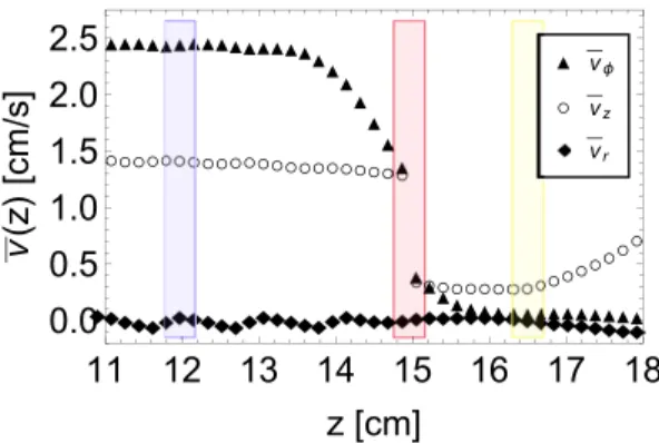
Fig. 9. Time averaged cylindrical components of the particle velocity as a function
of the axial position. The 3 highlighted sections correspond to the first 3 positions of Table 3: z0in blue, z1in red and z2in yellow. (For interpretation of the references to
colour in this figure legend, the reader is referred to the web version of this article.)
Since the contact law is unsuitable for modelling the high-pressure region close to the gap, we considered data up to point z2.
For the mean velocity we exploited the cylindrical symmetry of the system, still undisturbed by the presence of the rolls, and observed the cylindrical components of the former defined as
vr(r; t) = v2xx+ vyy
x2+ y2 v0(r; t) =
vxy − vyx
2
x2+ y2
.
(12)According to our definition, the angular component of the veloc-ity v0(r; t) has a positive sign when it is concurrent with the screw
rotation. InFig. 9we plotted the time average of the particles velocity components as a function of their position along the⃗z axis.
The mean radial component of the velocity is roughly zero both inside the conveyor case and in the first part of the compaction region up to z2(in yellow inFig. 9). From this point onwards, its value
is constantly negative, even if its magnitude is much smaller than the axial component, due to the pressure exerted by the rolls pushing the particles towards the⃗y = 0 plane. The angular component has a constant value inside of the screw barrel, as expected (e.g., at z0
high-lighted in blue). Its value starts to rapidly decrease close to the inlet region z1(in red inFig. 9) and approaches zero at z
>
z2. Althoughthe mean velocity along the feeding direction is constant along the entire screw length, it decays abruptly as soon as the particles are affected by back pressure due to the bulk effect in the first section of compaction region z1
<
z<
z2. From z2onwards, the mean axialvelocity constantly increases due to the combined effect of the pres-sure on particles exited by the conveyor and the rolls drag. Therefore, on average, the axial component of velocity is dominant inside the compaction region, while inside the screw barrel, far enough from the inlet, the flow is uniform with no net transport in the radial direction. The flow in the screw barrel can be compared with the experimental findings in [41]by means of X-ray penetration. The axial flow of the tracer particles observed in[41]is constant along
Fig. 10. Mean Cartesian component vx(r; t) of the particle velocity along 3 axial
sections as a function of time. The data correspond to the axial positions highlighted inFig. 9with the same colour code. The component vy(r; t) has the same periodic
behaviour, with a phase difference of p/2. (For interpretation of the references to colour in this figure legend, the reader is referred to the web version of this article.)
Fig. 11. Interpolation kernel proposed by Keys [42].
the screw length, with small oscillations when the powder meets the screw blade edge. These oscillations are factored out in our analy-sis because we averaged along the whole screw section. The radial motion of the tracer particles observed in the referenced paper is also shown to be almost negligible, and concentrated mainly around the screw blade edge. This is also consistent with our model, predicting an almost negligible mean radial velocity inside the barrel.
A much more detailed picture emerges if we analyze the flow as a function of time. To monitor the particle movement, we observed the Cartesian components of the mean velocity along the planes z0,
z1and z2. While the axial component of velocity evaluated as such
is roughly constant, the movement of particles coplanar to these sections is periodic in time. The velocity component vx(t) as a
func-tion of time along 5 screw rotafunc-tions is plotted inFig. 10. The velocity
vx(t) oscillates simultaneously with the same period TSof the screw.
Interestingly, this oscillation also persists inside of the compaction
region (yellow data points) and is likely to be responsible for the inhomogeneity of the powder bulk prior to compaction. The same oscillatory behaviour of the particles inside of the compacted region has been observed experimentally in[2]. It is this inhomogeneity that leads to the observed anisotropy in the compacted ribbon, as the following sections explain with the help of Finite Element modelling.
4. From CG to FEM
In order to implement DEM results into the FEM model, several steps are performed using MATLAB ®. First, the function “ndgrid” is being called in order to define a new rectangular grid in N-D space, which represents the FEM inlet mesh.
In the output [x, y] = ndgrid(xmin: hx : xmax, ymin: hy : ymax), the
coordinates of the (i, j)-th node are (xi, yi) = (xmin+ (i − 1)hx, ymin+
( j − 1)hy). Now that the new grid is formed to represent the FEM mesh, the DEM data is transferred. This is done via the “Interp2” function, which returns interpolated values of the DEM grid into the new FEM grid. The interpolated value at a query point is based on a cubic interpolation of the values at neighbouring grid points in each respective dimension.
For an equally spaced data, most interpolation functions are in the following form:
g(x) =)
k
cku(x − xk) (13)
where the sampled data is described as ck= f(xk) for a given sampled
function f at an interpolation node xkand u is the cubic
interpola-tion kernel. For convenient reasons, the distance between the point to be interpolated and the grid point being considered is defined as
s = (x − xk). The following cubic convolution interpolation kernel
(Eq. (14)), proposed by Keys[42], is symmetric and defined by piece-wise cubic polynomials in the intervals |s| ≤ 1 and 1
<
|s| ≤ 2. For |s|>
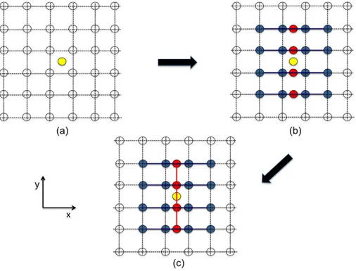
2, the kernel is zero. This kernel offers a third-orderFig. 12. Schematic illustration of the Bicubic convolution interpolation procedure. a) Initial point to be interpolated, b) first interpolation step along the x-direction. c) Final
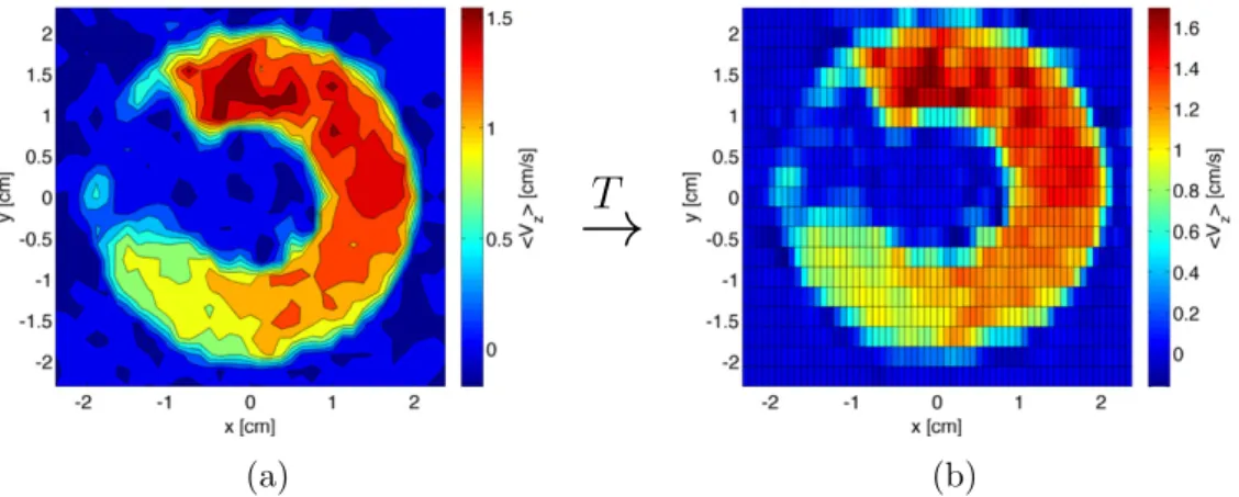
Fig. 13. Plot of velocity field and the transition from CG result to FEM inlet boundary condition for t∗= 0. Axial velocity component¯vzvalues for a) DEM coarse graining result
and b) corresponding FEM inlet nodes.
convergence and guaranteed superiority to nearest-neighbor (first order) and linear interpolation (second order)[43].
u(s) = ⎧ ⎪ ⎪ ⎨ ⎪ ⎪ ⎩ 3 2|s|3−52|s|2+ 1 |s| ≤ 1 −1 2|s|3+52|s|2− 4|s| + 2 1
<
|s| ≤ 2 0 |s|>
2 (14)Fig. 11 illustrates the one-dimensional case, interpolating the value x from the discrete points f(xk) using the cubic kernel. The
ker-nel function u(s) is centred at point x, the location of the point to be interpolated. The interpolated value g(x) is the weighted sum of the discrete neighbouring points (2 to the left and 2 to the right) scaled by the value of interpolation function at those points.
For two-dimensional interpolation (i.e., Bicubic interpolation), the one-dimensional function is applied in both directions. It is a sep-arable extension of the one-dimensional interpolation function. The Bicubic interpolation algorithms interpolate from the nearest sixteen mapped source pixels. Obtaining an interpolated value for a given point (yellow) is done in two steps. First (Fig. 12b), an interpolation is done along the x-direction (red points) using the 16 grid samples (blue points). The following step (Fig. 12c) is interpolating along the
y-direction (red line) using the interpolated points from the previous step.
The above algorithm is applied to the DEM CG data at each time interval Dt during a screw period, resulting in a total of 124 matri-ces of 61 × 20 (i.e., 1220 elements) corresponding to the FEM inlet nodes (Fig. 4a). The velocity values for each absolute time t∗are
then represented as an array in a separate file.Fig. 13illustrates the previously described steps of constructing a new grid, which cor-relates to the FEM mesh and interpolates the values from the DEM results.
The new interpolated data is then implemented as a FEM nodal velocity boundary condition in Abaqus/Explicit using an external user-defined VDISP Fortran subroutine. At each absolute time t∗, the
VDISP subroutine is being called and assigns the corresponding inter-polated velocity values from the previously saved data file into the FEM model in a chronological order to the predefined inlet nodes (Fig. 14.).
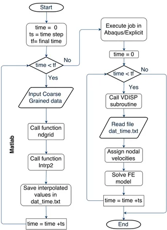
The flowchart in Fig. 15describes the entire procedure imple-mented in this work. The first part describes the numerical transition method used to bridge the gap between the DEM coarse grained results and the FEM inlet nodes. The second step contains the FEM explicit simulation using the VDISP subroutine in order to implement the DEM data and solve the FEM model for each time step.
Fig. 14. Schematic illustration of the procedure assigning axial inlet velocity interpolated values into the FEM model. The red arrows show the direction in which values are read
in the data file and being assigned into the FEM back nodes. (For interpretation of the references to colour in this figure legend, the reader is referred to the web version of this article.)
Fig. 15. Flow chart block diagram describing the FEM simulation using CG results.
5. Results and discussion
Results obtained by DEM simulation (Section 3), showed that the flow of powder being conveyed to the rolls, varies in velocity due to the oscillation of the screw. This is in fact the main cause attributed to the inhomogeneity of the compacted ribbon, resulting in a “snake”-wise light transmission pattern [2]. Our results demonstrates the importance of combining DEM & FEM methods to obtain a more realistic model of the process.
5.1. Transition From DEM (CG) to FEM
In the previous section, the multi-scale approach was described in order to investigate the behaviour of granular material in roll
compaction, by combining DEM at the micro scale into the FEM macro scale level.Fig. 16visualizes the result of the numerical transi-tion method, which was used to gap between the different scales and used as input data in FEM modelling. By comparing the axial veloc-ity component¯vzin the FEM inlet nodes (Fig. 16) with the CG results
(Fig. 8), it can be seen that feeding velocity field values and pat-tern are almost identical with some discrepancies due to the counter pressure from the rolls (except for t∗ = 0 inFig. 16a). Therefore,
it is possible to successfully implement the DEM data into the FEM, and to represent the velocity of the powder entering the compaction region.
5.2. DEM & FEM combined simulation
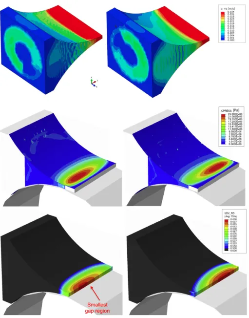
By implementing the CG DEM results into the FEM, a numerical study on the effect of the screw blade position and the inhomoge-neous inlet feeding velocity on the roll compaction process was con-ducted. The resulting contact pressure and relative density (Fig. 17) are distributed non-homogeneously in the minimum gap region and vary with time as a result of the inlet feeding velocity. The maximum contact roll pressure and relative density positions in the minimum gap region vary with simulation time along the ribbon’s width. It can be noted that the 3D axial velocity plot does not correspond to the pressure and density values at the minimum gap due to the fact that the influence of the inlet velocity takes effect only at a later stage. This means that, due to the distance between the inlet region and the minimum gap region, there is a certain phase shift between the sinu-soidal pattern of the inlet velocity and the contact roll pressure and relative density.
In order to evaluate and quantify this variation during the process and consequently on a compacted ribbon, the values were monitored at two different positions with a distance of 5 mm from the left and right side seals (Fig. 18). Initially, the values of relative density and contact pressure are increasing gradually as powder is being deliv-ered in between the rolls. At around t∗ = 3 s, the roll compaction
reaches a steady-state condition, where the mean values of the rel-ative density and of the roll pressure at the minimum gap region remain constant.
Results obtained with our combined approach showed that the inlet feeding velocity has a direct effect on the resulting pres-sure and density distribution. Fig. 18clearly shows the variation of the value within simulation time. For a specific time, the con-tact pressure and relative density values at one side of the rib-bon are higher with respect to the other. Moreover, a sinusoidal pattern of the roll pressure and relative density during com-paction is observed, having a period equal to the screw rotation period.
Fig. 16. 3D plots of the axial velocity component ¯vzin the FEM model (right seal removed for better visualisation) for 3 screw positions, with a counter-clockwise rotation. The
Fig. 17. 3D plots of FEM modelled parameters for 2 time steps: t∗= 2.35 s (left column) and t∗= 2.9 s (right column). The depicted values are: powder axial velocity (top row),
contact pressure (middle row) and relative density (bottom row) at the outlet of the compaction region.
Due to numerical reasons, the results are obtained and plot-ted only for the material which is still in contact with the roll, up to the narrowest gap region[15]. Therefore, in order to illustrate the resultant roll compacted ribbon, multiple sliced snapshot at the gap region were taken at intervals of Dt = 0
.
05 s and assembled together. As can be seen clearly inFig. 19, higher powder feeding rate in one side resulted in higher contact pressure and relative density on the same side under the rolls. This can be explain by transport-ing higher amount of mass into one side, thus increastransport-ing the nip angle which will ultimately result in higher compaction force and density.6. Conclusions
Roll compaction is a complex process involving two main parts, powder conveying using a screw feeder and compaction between two counter rotating rolls, where the powder undergoes
large deformation. In this work, a combined DEM-FEM multi-scale approach was developed in order to investigate the behaviour of granular material in roll compaction.
DEM was used to model the flow of granular material through the screw conveyor into the compaction zone. The DEM simula-tion was successfully used to model the behaviour of particles in a screw feeder and to obtain the highly inhomogeneous (although periodic in time) velocity field at the interface between the screw feeder and the compaction region. Then, FEM was applied to sim-ulate the powder compaction in between the rolls and to study the effect of the inhomogeneous inlet feeding velocity due to the screw feeder. The combined DEM-FEM methodology clearly shows the resultant inhomogeneous roll contact pressure and relative den-sity over the rolls width, resulting in a “snake-wise” pattern over time. This behaviour is reflected in an inhomogeneously compacted ribbon. Moreover, the sinusoidal pattern of the roll pressure and rel-ative density during roll compaction has a period equal to the screw rotation time.
Fig. 18. Plots of the a) roll contact pressure and b) relative density at two positions 5
mm from both edges with respect of time. The highlighted region is the time domain used for plottingFig. 19.
Combining both DEM and FEM methods to model the roll com-paction process allows us to take advantage of the strength of both methods in order to describe complex processes, and enables us to achieve a more realistic model of both the process itself and of the final product quality. The methodology proposed can be used to study how process parameters, such as screw and roll speeds, will
likely affect the ribbon density and homogeneity. In addition, this coupled approach can be a useful tool to guide future design optimi-sations, with the aim to diminish the effect of the screw driven flow on the compaction final product.
Acknowledgments
This project has received funding from the European Union’s Seventh Framework Programme for research, technological develop-ment and demonstration under grant agreedevelop-ment no. 316555.
References
[1] O. Simon, P. Guigon, Correlation between powder-packing properties and roll press compact heterogeneity, Powder Technol. 130 (2003) 257–264.http://dx. doi.org/10.1016/S0032-5910(02)00202-4.
[2] P. Guigon, O. Simon, Roll press design - influence of force feed systems on com-paction, Powder Technol. 130 (2003) 41–48. http://dx.doi.org/10.1016/S0032-5910(02)00223-1.
[3] A. Roberts, The influence of granular motion on the volumetric performance of enclosed screw conveyors, Powder Technol. 104 (1999) 56–67.http://dx.doi. org/10.1016/S0032-5910(99)00039-X.
[4] L. Pezo, A. Jovanovi´c, M. Pezo, R. ˇColovi´c, B. Lonˇcar, Modified screw conveyor-mixers - discrete element modeling approach, Adv. Powder Technol. 26 (2015) 1391–1399.http://dx.doi.org/10.1016/j.apt.2015.07.016.
[5] Q. Hou, K. Dong, A. Yu, DEM study of the flow of cohesive particles in a screw feeder, Powder Technol. 256 (2014) 529–539.http://dx.doi.org/10.1016/ j.powtec.2014.01.062.
[6] O. Imole, D. Krijgsman, T. Weinhart, V. Magnanimo, B.C. Montes, M. Ramaioli, S. Luding, Reprint of “Experiments and discrete element simulation of the dos-ing of cohesive powders in a simplified geometry”, Powder Technol. 293 (2016) 69–81.http://dx.doi.org/10.1016/j.powtec.2015.07.052.
[7] P. Moysey, M. Thompson, Modelling the solids inflow and solids conveying of single-screw extruders using the discrete element method, Powder Technol. 153 (2005) 95–107.http://dx.doi.org/10.1016/j.powtec.2005.03.001. [8] J.R. Johanson, A rolling theory for granular solids, J. Appl. Mech. 32 (4) (1965)
842–848.http://dx.doi.org/10.1115/1.3627325.
[9] G. Reynolds, R. Ingale, R. Roberts, S. Kothari, B. Gururajan, Practical applica-tion of roller compacapplica-tion process modeling, Comput. Chem. Eng. 34 (7) (2010) 1049–1057.http://dx.doi.org/10.1016/j.compchemeng.2010.03.004. [10] M. Bi, F. Alvarez-Nunez, F. Alvarez, Evaluating and modifying Johanson’s
rolling model to improve its predictability, J. Pharm. Sci. 103 (2014) 2062–2071. http://dx.doi.org/10.1002/jps.24012.
Fig. 19. Multiple sliced snapshots of the a) relative density and b) contact pressure values obtained by the combined DEM-FEM simulations at the minimum gap region between
[11] R.T. Dec, A. Zavaliangos, J.C. Cunningham, Comparison of various modeling methods for analysis of powder compaction in roller press, Powder Technol. 130 (2003) 265–271.http://dx.doi.org/10.1016/S0032-5910(02)00203-6. [12] J.C. Cunningham, Experimental studies and modeling of the roller compaction
of pharmaceutical powders, Strain (July) (2005) 267.
[13] A. Michrafy, H. Diarra, J.A. Dodds, M. Michrafy, L. Penazzi, Analysis of strain stress state in roller compaction process, Powder Technol. 208 (2011) 417–422. http://dx.doi.org/10.1016/j.powtec.2010.08.037.
[14] A.R. Muliadi, J.D. Litster, C.R. Wassgren, Modeling the powder roll compaction process: comparison of 2-D finite element method and the rolling theory for granular solids (Johanson’s model), Powder Technol. 221 (2012) 90–100.http:// dx.doi.org/10.1016/j.powtec.2011.12.001.
[15] A.R. Muliadi, J.D. Litster, C.R. Wassgren, Validation of 3-D finite element analysis for predicting the density distribution of roll compacted pharmaceuti-cal powder, Powder Technol. 237 (2013) 386–399.http://dx.doi.org/10.1016/j. powtec.2012.12.023.
[16] A. Mazor, L. Perez-Gandarillas, A. de Ryck, A. Michrafy, Effect of roll compactor sealing system designs: a finite element analysis, Powder Technol. 289 (2016) 21–30.http://dx.doi.org/10.1016/j.powtec.2015.11.039.
[17] A. Michrafy, H. Diarra, J.A. Dodds, M. Michrafy, Experimental and numerical analyses of homogeneity over strip width in roll compaction, Powder Technol. 206 (1–2) (2011) 154–160.http://dx.doi.org/10.1016/j.powtec.2010.04.030. [18] J.C. Cunningham, D. Winstead, A. Zavaliangos, Understanding variation in
roller compaction through finite element-based process modeling, Computers and Chemical Engineering 34 (7) (2010) 1058–1071.http://dx.doi.org/10.1016/ j.compchemeng.2010.04.008.
[19] Y. Liu, C. Wassgren, Modifications to Johanson’s roll compaction model for improved relative density predictions, Powder Technol. 297 (2016) 294–302. http://dx.doi.org/10.1016/j.powtec.2016.04.017.
[20] D. Choi, N. Kim, K. Chu, Y. Jung, J. Yoon, S. Jeong, Material properties and compressibility using Heckel and Kawakita equation with commonly used pharmaceutical excipients, J. Pharm. Investig. 40 (4) (2010) 237–244. [21] H. Hiestand, D. Smith, Indices of tableting performance, Powder Technol. 38
(2) (1984) 145–159.http://dx.doi.org/10.1016/0032-5910(84)80043-1. [22] P. Cundall, O. Strack, A discrete numerical model for granular assemblies,
Géotechnique 29 (1979) 47–65.http://dx.doi.org/10.1680/geot.1979.29.1.47. [23] H. Hertz, A discrete numerical model for granular assemblies, J. Reine Angew.
Phys. 92 (1882) 156.
[24] N. Brilliantov, F. Spahn, J. Hertzsch, T. Pöschel, A model for collisions in gran-ular gases, Phys. Rev. E 53 (1996) 5382.http://dx.doi.org/10.1103/PhysRevE.53. 5382.
[25] K. Watanabe, H. Tanaka, Direct observation of medium-range crystalline order in granular liquids near the glass transition, Phys. Rev. Lett. 100 (2008) 158002(4).http://dx.doi.org/10.1103/PhysRevLett.100.158002.
[26] R. Sánchez, I. Romero-Sánchez, S. Santos-Toledano, A. Huerta, Polydisper-sity and structure: a qualitative comparison between simulations and granular systems data, Rev. Mex. Fis. 60 (2014) 136–141.
[27] Y. Zhou, B. Xu, A. Yu, Numerical investigation of the angle of repose of monosized spheres, Phys. Rev. E 64 (2001) 021301.http://dx.doi.org/10.1103/ PhysRevE.64.021301.
[28] R. Roberts, R. Rowe, P. York, Poisson’s ratio of microcrystalline cellulose, Int. J. Pharm. 105 (1994) 177–180.
[29] B. Hancock, S. Clas, K. Christensen, Micro-scale measurement of the mechan-ical properties of compressed pharmaceutmechan-ical powders. 1: the elasticity and fracture behavior of microcrystalline cellulose, Int. J. Pharm. 209 (2000) 27–35. [30] B. Latella, S. Humphries, Young’s modulus of a 2.25Cr-1Mo steel at ele-vated temperature, Scr. Mater. 51 (2004) 635–639.http://dx.doi.org/10.1016/j. scriptamat.2004.06.028.
[31] H. Ledbetter, Stainless-steel elastic constants at low temperatures, J. Appl. Phys. 52 (1981) 1587.3.
[32] C. Kloss, C. Goniva, A. Hager, S. Amberger, S. Pirker, Models, algorithms and validation for opensource DEM and CFD-DEM, Prog. Comput. Fluid Dyn. 12 (2012) 140–152.http://dx.doi.org/10.1504/PCFD.2012.047457.
[33] P.U. Dassault Systems, ABAQUS Documentation, 2014.
[34] D.J. Benson, S. Okazawa, Contact in a multi-material Eulerian finite element formulation, Comput. Methods Appl. Mech. Eng. 193 (2004) 4277–4298.http:// dx.doi.org/10.1016/j.cma.2003.12.061.
[35] S. Helwany, Applied Soil Mechanics With ABAQUS, 2007.
[36] L.H. Han, J. a. Elliott, a. C. Bentham, a. Mills, G.E. Amidon, B.C. Hancock, A modified Drucker-Prager Cap model for die compaction simulation of pharma-ceutical powders, Int. J. Solids Struct. 45 (2008) 3088–3106.http://dx.doi.org/ 10.1016/j.ijsolstr.2008.01.024.
[37] I. Goldhirsch, Stress, stress asymmetry and couple stress: from discrete parti-cles to continuous fields, Granul. Matter 12 (2010) 239–252.http://dx.doi.org/ 10.1007/s10035-010-0181-z.
[38] T. Weinhart, A. Thornton, Closure relations for shallow granular flows from particle simulations, Granul. Matter 14 (2012) 531–552.http://dx.doi.org/10. 1007/s10035-012-0355-y.
[39] L. Lucy, A numerical approach to the testing of the fission hypothesis, Astron. J. 82 (1977) 1013–1024.
[40] T. Weinhart, R. Hartkamp, A. Thornton, S. Luding, Coarse-grained local and objective continuum description of three-dimensional granular flows down an inclined surface, Phys. Fluids 25 (2013) 070605.26.http://dx.doi.org/10.1063/ 1.4812809.
[41] K. Uchida, K. Okamoto, Measurement of powder flow in a screw feeder by X-ray penetration image analysis, Measurement Science and Technology 17 (2006) 419–426.http://dx.doi.org/10.1088/0957-0233/17/2/025.
[42] R.G. Keys, Cubic convolution interpolation for digital image processing, IEEE Trans. Acoust. Speech Signal Process. 29 (6) (1981) 1153–1160.
[43] J.A. Parker, R.V. Kenyon, D.E. Troxel, Comparison of interpolating methods for image resampling, IEEE Trans. Med. Imaging 2 (1) (1983) 31–39. ISSN 0278-0062.http://dx.doi.org/10.1109/TMI.1983.4307610.
![Fig. 5. Density-dependant Drucker-Prager Cap model [16].](https://thumb-eu.123doks.com/thumbv2/123doknet/11586630.298421/7.892.64.404.857.1123/fig-density-dependant-drucker-prager-cap-model.webp)