Noise-Corrected Estimation of Complex Modulus in Accord With Causality and Thermodynamics: Application to an Impact Test.

(1)

HAL Id: hal-00968927

https://hal.archives-ouvertes.fr/hal-00968927

Submitted on 4 Apr 2014

HAL is a multi-disciplinary open access archive for the deposit and dissemination of sci-entific research documents, whether they are pub-lished or not. The documents may come from teaching and research institutions in France or abroad, or from public or private research centers.

L’archive ouverte pluridisciplinaire HAL, est destinée au dépôt et à la diffusion de documents scientifiques de niveau recherche, publiés ou non, émanant des établissements d’enseignement et de recherche français ou étrangers, des laboratoires publics ou privés.

Noise-Corrected Estimation of Complex Modulus in

Accord With Causality and Thermodynamics:

Application to an Impact Test.

Pierre Collet, Gérard Gary, Bengt Lundberg

To cite this version:

Pierre Collet, Gérard Gary, Bengt Lundberg. Noise-Corrected Estimation of Complex Modulus in Accord With Causality and Thermodynamics: Application to an Impact Test.. Journal of Applied Mechanics, American Society of Mechanical Engineers, 2013, 80 (011018-1), pp.JANUARY 2013. �10.1115/1.4007081�. �hal-00968927�

(2)

Noise-corrected Estimation of Complex Modulus in

Accord With Causality

and

Thermodynamics:

Application to an Impact test

P. Collet

1

, G. Gary

2

, B. Lundberg

2,3

1

Centre de Physique Théorique, CNRS UMR 7644, Ecole Polytechnique, 91128 Palaiseau, France

2

Laboratoire de Mécanique des Solides, CNRS UMR 7649, Ecole Polytechnique, 91128 Palaiseau, France

3

The Ångström Laboratory, Uppsala University, Box 534, SE-751 21 Uppsala, Sweden

Background. Methods for estimation of the complex modulus generally produce data

from which discrete results can be obtained for a set of frequencies. As these results are

normally afflicted by noise, they are not necessarily consistent with the principle of

causality and requirements of thermodynamics.

Method of Approach: A method is established for noise-corrected estimation of the complex modulus, subject to the constraints of causality, positivity of dissipation rate and

reality of relaxation function, given a finite set of angular frequencies and corresponding

complex moduli obtained experimentally. Noise reduction is achieved by requiring that

two self-adjoint matrices formed from the experimental data should be positive

semi-definite.

Results: The method provides a rheological model that corresponds to a specific

configuration of springs and dashpots. The poles of the complex modulus on the positive

imaginary frequency axis are determined by a subset of parameters obtained as the

(3)

obtained from a least squares fit. If the set of experimental data is sufficiently large, the

level of refinement of the rheological model is in accordance with the material behaviour

and the quality of the experimental data. The method was applied to an impact test with a

Nylon bar specimen. In this case, data at the 29 lowest resonance frequencies resulted in

a rheological model with 14 parameters.

Conclusions: The method has added improvements to the identification of rheological models as follows: (1) Noise reduction is fully integrated. (2) A rheological model is

provided with a number of elements in accordance with the complexity of the material

behaviour and the quality of the experimental data. (3) Parameters determining poles of

the complex modulus are obtained without use of a least squares fit.

Keywords : Mechanical properties of materials, constitutive modeling of materials, impact, wave propagation.

(4)

1 Introduction

A variety of methods for identification of viscoelastic materials have been proposed and used since long. Such methods for estimation of complex-valued

frequency-dependent material parameters such as the complex modulus, generally produce data from which values of these parameters can be obtained for a set of discrete frequencies. Commercially available machines for dynamic mechanical analysis (DMA) [1] as well as specialized and laboratory-specific set-ups are used. Some make use of forced or free vibrations of a structure such as a bar, while others involve impact, waves and various transient effects.

Garrett [2] used a method based on acoustic resonance in a study of the temperature dependency of the Young’s modulus. A similar method was proposed by Guo and Brown

[3] for viscoelastic materials. With this method, a 1D theoretical model is fitted to

experiments on frequency intervals of finite length which provides values of the complex

modulus at discrete frequencies. Some methods [4] make use of random excitation at one end of a beam and measurement of acceleration at the other end. With the assumption of

1D viscoelastic behaviour, the complex Young’s modulus is derived from the amplitude

ratio and phase shift between acceleration and excitation. Pintelon et al. [5] proposed a

method which takes dispersion into account by use of Love’s model [6]. They used a

resonant frequency method in conjunction with forced vibration. Their method is based

on measurement of the force applied at one end of a bar and the axial displacement at a

given section. Noise reduction is provided by repetition of measurements and

identification of a rheological model. Waves in bars generated by impact have been used to determine the viscoelastic properties of materials by, e.g., Blanc [7, 8], Lundberg and

(5)

Blanc [9], Lundberg and Ödeen [10], Hillström et al. [11], Othman [12], and Mousavi et

al. [13].

It is not always ensured that the real and imaginary parts of the complex modulus

are consistent with the principle of causality. One way to achieve such consistency is to

express them in terms of a rheological model constituted by linear springs and dashpots

[5, 14]. An alternative way consists in making sure that the complex modulus is

consistent with the Kramers-Kronig relations. Another fundamental constraint on the

complex modulus comes from the second principle of thermodynamics: the dissipation

per cycle must be positive for any harmonic load. Furthermore, the relaxation function,

which is the inverse Fourier transform of the complex modulus, must be real. See, e.g.,

Landau and Lifchitz [15, 16] about these constraints.

In Section 2 we present a method for noise-corrected estimation of the complex modulus of a viscoelastic material, subject to the constraints of causality, positivity of dissipation and reality of relaxation function, given an experimental set of frequencies and corresponding values of the complex modulus. It provides the structure, the number and type of elements, and the parameters of a rheological model and is based on results from different areas of mathematics and physics. As far as we know, similar results have not been combined previously into a practical method for producing a noise-corrected rheological model of suitable complexity that satisfies the above mentioned constraints. The estimation method can be used in conjunction with any test method from which a set of frequencies and corresponding values of the complex modulus can be obtained. In Section 3 the use of the method will be illustrated with such data obtained by impacting a Nylon bar specimen and observing its response at its resonance frequencies.

(6)

2 Estimation

Method

2.1 Theory. According to Boltzmann’s model of viscoelastic materials, the

relation between stress 

 

t and strain 

 

t is given by the convolution

 

   

t s ds dt d s G = t σ



   0 (1)

of the stress relaxation function G

 

t and the strain rate d / dt, where t is time (e.g., [17]). After Fourier transformation, this relation becomes

     

ω =E ω ω

σˆ ˆ , (2)

where E

 

ωiGˆ

 

 is the complex modulus, Gˆ

 

 is the Fourier transform of G

 

t and  is the angular frequency.

The complex modulus must satisfy the three constraints of causality, positivity of

the dissipation rate and reality of the relaxation function. The problem to be considered is

that of finding a noise-corrected complex modulus E

 

ω , subject to these constraints, given a finite set of angular frequencies ω₁,,ω_n and corresponding complex moduli

n

E ,

E₁  obtained experimentally.

The constraint of causality implies the Kramers-Kronig relations that connect the

(7)

can be estimated accurately at a sufficient number of frequencies, these relations can be

used to estimate the other part. For several experimental methods based on wave

propagation, e.g. [18, 19], and the one to be presented in this paper, such a procedure

does not work as the experimental noise is rather uniformly distributed over the real and

imaginary parts of the complex modulus. Furthermore, results for the complex modulus

can be obtained only for a relatively small set of frequencies with the experimental

method of this paper. Here, therefore, we adopt the approach of estimating

simultaneously the real and imaginary parts of the complex modulus. This will also allow

us to extend the results to regions without measurements, especially at low frequencies.

The constraints of causality and of positivity of the dissipation rate [15-17, 20] are

equivalent to requiring that the function E

 

ω be analytic in the lower half plane and that its imaginary part be positive on the positive real axis, respectively. The constraint of

reality of the relaxation function is equivalent to the requirement E

 

ω =E

 

ω . Here we will use the stronger constraint of complete monotonicity of the relaxation function as

proposed by Hanyga [17] and Bouleau [21] and derived by Beris and Edwards [22] for

fluids. This constraint, which essentially means that the relaxation function and its

derivatives must be monotone, is satisfied by most rheological models [17]. To which

extent it holds for a particular real material can be verified from experimental data.

The property of complete monotonicity of the relaxation function implies that this

function is the Laplace transform of a positive function (the Bernstein-Widder Theorem,

see [17]). This means that the complex modulus E

 

ω is the sum of a linear function and a Stieltjes transform. More precisely, there exist two parameters ₀0 and ₀ 0, and a function h

 

s 0, defined on the positive real axis such that

(8)

 



_



 

0 0 0 i i ds ω + s s h ω + = ω E   . (3)

Such functions E

 

ω are analytic outside the positive imaginary axis of the complex ω plane and they satisfy the three constraints. Thus, they are analytic in the lower half plane

and therefore satisfy the constraint of causality; their imaginary part is positive on the

positive real axis and therefore the constraint of positiveness of the dissipation rate holds.

Finally, the constraint of reality of the relaxation function is satisfied as E

 

ω =E

 

ω . It should be noted that the function h

 

s can have singularities such as delta functions.

In order to check whether experimental data are of the form of Eq. (3), in particular

for the purpose of determining the constants ₀ and ₀, and the function h, it is convenient to apply the transformation

 

E

 

_zz =

z

f  i . (4)

It has the representation

 

ds z s s g + = z f



 0  , (5) with

(9)

 

   

h_ss + s du u u h = s g     



 0 0  , (6)

where

 

s is a delta function at the origin, and g

 

s =0 for s<0. As the static complex modulus

 

ds s s h = E



  0 0 0  (7)

is positive and finite, the function f

 

z is analytic except on the positive real axis, and positive on the negative real axis.

The problem of finding a function f

 

z with the representation (5) given its values for finitely many z was studied in detail by Krein and Nudelman [23]. Some of their

results, when formulated for the complex modulus E

 

ω , are as follows. From the values

1

E , E₂, …, E of the function _n E

 

ω at n angular frequencies ₁, ₂, …, _n one can form two matrices with elements

  k j k j k j, _ω + ω E E = M 1 i 

 



s ωj





s+ ωk



ds s h + = i i 0 0 



  , (8)   k j k k j j k j, _ω + ω E E = M 2 /  /

 









. i i 0 0



  j k k j s ω s+ ω ds s s h + ω ω E = (9)

(10)

It can be verified that the matrix M 1 is positive semi-definite. In particular, it is

self-adjoint with non-negative eigenvalues (recall that ₀ and h are non-negative). The same properties hold for M 2 since E

 

0 >0. If one of the matrices M 1 or M 2 has a zero eigenvalue, the function E

 

ω is completely determined and is a rational fraction (see [23] and below). However, the occurrence of a zero eigenvalue is not a necessary

consequence of general principles, and if none of the matrices M 1 and M 2 has a zero

eigenvalue, the function E

 

ω cannot be completely determined from the data. We refer to Krein Nudelman (1998) for more details.

Assume now that a is an eigenvector corresponding to a zero eigenvalue of M 1 .

Then, since M 1a= 0,we also have a,M 1a =0, i.e.,

 

0. i 2 1 0 2 1 0 _ω ds= + s a s h + a n = k k k n = k k            

_



_

_

 (10)

Since both terms in the left member are non-negative, they must vanish. In particular, the

function h

 

s must be a linear combination



_l



p l

l ss



_  

1

with coefficients _l 0 of delta functions 



ss_l



at the positive zeros s₁,,s_p



p<n



of the rational function



n = k k k ω + s a 1 i . (11)

(11)

For the complex modulus given by Eq. (3) this implies the model

 



_

l=p = l l l ω + s γ iω + = ω E 1 0 0 i   , (12)

where 0₀  and ₀, γ₁, γ₂, …, γ are non-negative. _p

The same considerations hold for the matrix M 2 and should lead to the same

model. If bis an eigenvector corresponding to a zero eigenvalue of M 2 , we deduce as

above that the function h

 

s must also be a linear combination with non-negative coefficients of delta functions at the positive zeros of the rational function



n = k k k ω + s b 1 i . (13)

In particular, we only need to consider the common positive zeros of the rational

functions (11) and (13). Moreover, if there are several linearly independent eigenvectors

corresponding to a zero eigenvalue, we get a set of positive zeros for each of them and

should keep only the ones which are common.

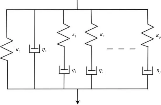
Equation (12) corresponds to the 2



p1



parameter rheological model shown in Fig. 1 consisting of p full Maxwell elements (each consisting of a spring and a dashpot in series) and two degenerated such elements (a spring, a dashpot) in parallel. The complex modulus represented by this model is

(12)

 

_

            p l l l l l p l l p l l l l E 1 2 0 1 0 1 0 0 i / / i i / i i                . (14)

The p1 stiffnesses ₀, ₁, … _p of the springs and the p1 viscosities ₀, ₁, … _p of the dashpots are related to the 2



p1



parameters and ₀, ₀, s₁, s₂, …, s , _p

1

γ , γ₂, …, γ of Eq. (12) by the relations _p



_   p l l l s 1 0 0    , l l l s    , 0  , 0 2 l l l s    . l1, 2,…..p (15)

The viscoelastic material represented by Eqs. (12) and (14) has asymptotic elasticity as E

 

0 ₀ is finite, but generally it does not possess instant elasticity. If ₀ and ₀ vanish, however, E

 

 ₀₁..._p is finite. Then, the material has also instant elasticity and qualifies as a solid [24].

It is noted that the points ω₁,,ω_n are strictly inside the analyticity domain of the function E

 

ω. This follows from Eq. (3) and makes the following approach robust compared to situations with data points on the boundary of the analyticity domain.

2.2 Implementation. From experiments, we obtain a finite set of angular

frequencies ω₁,,ω_n and corresponding complex moduli E₁,E_n . By use of these experimental data we form the two matrices M(1)_j,_k and M(2)_j,_k given by the first equalities

(13)

and only if all their eigenvalues are non-negative. However, experiments commonly

result in some slightly negative eigenvalues. In the experimental part of this paper, for

example, the modulus of the smallest negative eigenvalue is typically a few tenths of a

percent of the largest positive eigenvalue. A likely explanation for such small violations

of the positive semi-definiteness is experimental noise. As advocated by Gu et al. [25] for a similar problem, the effects of such noise can be reduced by searching the smallest

possible corrections of ω₁,..., ω and _n E , …, ₁ E which restore the non-negativeness of _n

all eigenvalues and establishing noise-corrected sets ω₁corr,..., ω and _ncorr E₁corr, …, E_ncorr. If at least one of the noise-corrected matrices  1corr

M and  2corr

M has a zero eigenvector, one forms the associated rational fraction (11) or (13) and finds its positive

zeros. This is repeated for the set of independent eigenvectors, if any, corresponding to

zero eigenvalues of both matrices. Then one keeps the common positive zeros s₁,,s_p

of all these rational fractions and obtains the model given by Eq. (12). In this model the

p positive parameters s₁,,s_p are known.

If the frequency range of interest does not extend far above that of the experimental data, ₀ 0, ₀ 0 and the p non-negative parameters γ₁, γ₂, …, γ_p are identified by a least square fit of the model to the noise-corrected data. If the material is required to possess instant elasticity, however, ₀ can be taken as zero while the remaining parameters are identified by a least square fit.

In this way, the method provides the structure, the number of elements and the

parameters of the rheological model. Normally, the number of elements is found to be

(14)

3 Impact

Test

Method

As stated in the Introduction, an experimental set of discrete angular frequencies and corresponding values of the complex modulus may be obtained with a variety of test methods, commercial as well as specialized and laboratory-specific. Here, as an example, they will be obtained by analysing the wave propagation in a Nylon bar specimen loaded through axial impact. The method is a slightly improved version of that used by Othman et al. [26].

3.1 Theory. Discrete values of the complex modulus E

   

 E iE

 

 will be obtained from the resonances of an impacted uniform bar specimen with density  and length l as shown in Fig. 2. At one end, x0, the bar is impacted axially by a striker that separates from the bar after the generation of a compressive primary pulse in

the bar. The other end of the bar, x , is free. The strain l _b

   

t  b,t is recorded at a distance a from the free end and b from the impacted end (abl). The primary pulse should be shorter than a2 so that there is no overlap in the measured strain of this pulse and the first pulse reflected from the free end. However, it should be much longer than

the diameter of the bar so that approximate 1D conditions prevail (wavelengths much

longer than the diameter of the bar [27].

In the frequency domain, the strain in the bar can be expressed as

   

_x _A _e   x _B

_{ }

 _e  x

(15)

where

   

   E 2 2  , 

     

  k  i  . (17)

Here, ˆ x

 

, is the Fourier transform of 

 

x,t , and A

 

 and B

 

 are complex amplitudes of waves travelling in the directions of increasing and decreasing x ,

respectively, k

 

 is the wave number and 

 

 is the damping coefficient. In order to determine an expression for the recorded strain ˆ1

   

 ˆ ,

b

b 

associated with the primary pulse alone, the amplitudes A and B are first determined

from Eq. (16) and the boundary conditions ˆ

   

0, ˆ₀  and B

 

 0 for a semi-infinite bar x0, where ˆ₀

 

 is the strain at the impacted end. With these amplitudes and xb inserted, Eq. (16) gives

 

 

 

   0 -i 1 ˆ ˆ b b e . (18)

The recorded strain ˆb

   

 ˆ b,

 _{associated with the complete train of pulses is}

determined similarly. First, the amplitudes A and B are determined from Eq. (16) and

the boundary conditions ˆ

 

0, ˆ₀

 

 and ˆ

 

l, 0 for the finite bar 0xl. With these amplitudes, and xb and lba inserted, Eq. (16) gives

 



 

_{   }

_    ˆ0 sin sin ˆ l a b   _. ₍₁₉₎

(16)

Dividing the members of Eq. (19) by those of Eq. (18) eliminates the strain

 



ˆ0 at the impacted end which normally cannot be measured. This slightly improves

the method previously used by Othman et al. [26]. Substituting  from the second of Eqs. (17) into the result, one gets the ratio ˆ_b

   

 /ˆ_b1  which gives

 

_{ }

 

_{ }

l kl a ka e b b b        2 2 2 2 2 2 1 2 sinh sin sinh sin ˆ ˆ     _. ₍₂₀₎

Resonance occurs at the angular frequencies _m, m 1, 2, … which correspond to 

the wave numbers, wavelengths and phase velocities

l m k k _m   , m l k_m m 2 2      ,    m l k c c m m m m    , m 1, 2, … (21)  respectively.

It is assumed that within the m:th resonance peak  _m/_m can be taken as directly proportional to angular frequency and c

 

 /k

 

 c_m can be taken as constant. By use of the third of Eqs. (21) we then obtain the relation k

 

 k_m/_m between wave number and angular frequency within the resonance peak. Inserting these

expressions for 

 

 and k

 

 into Eq. (20) we get

 



_



_



_

_



m m m m m m m m b b b l l k a a k e m m                  / sinh / sin / sinh / sin ˆ ˆ 2 2 2 2 / 2 2 1 2     _, ₍₂₂₎

(17)



m 1, 2, …

within the m:th resonance peak. In this relation, the spectra ˆ_b

 

 2 and ˆ1_b

 

 2 can be determined experimentally.

For each resonance m 1, 2, …, the resonance frequency  _m and damping coefficient _m can be estimated by minimizing the difference between the resonance peaks represented by the left and right members of Eq. (22). From _m and m, an experimental phase velocity c can be obtained by use of the third of Eqs. (21). Finally, _m

by use of the dispersion relation (17) and the first of Eqs. (21), the complex modulus

m

E at each resonance frequency can be obtained as

2     m m m= E    , _m α_m l m = ξ  i , m 1,  2, …. (23)

3.2 Experimental Set-up and Procedure. Impact tests were carried out with a

Nylon bar specimen of length l3 045 mm, diameter 10.2 mm, and density 1 149 kg/m3. Two pairs of strain gauges, one axial and one circumferential, were located at a

distance of a1 731 mm from the free end and b1 314 mm from the impacted end. In order to minimise the effects of friction, the bar was suspended horizontally by means of

nine regularly spaced strings with length 300 mm. With this arrangement, the period of

oscillation of the system was about one second, which is much longer than the test

(18)

the bar, and its impact velocity was 3.7 m/s. The strain was recorded with 500 kHz

sampling frequency, and the signal vanished completely before the end of the recording

window.

Results were evaluated up to 8 kHz. With a phase velocity expected to be higher

than 1 500 m/s at this frequency, the shortest significant wave length was estimated to be

greater than 0.19 m. This wave length is much larger than the diameter 0.01 m of the bar,

which means that 3D effects can be neglected as assumed in Section 3.1.

4 Results

and

Discussion

The estimation method presented provides a model for the complex modulus

corresponding to that shown in Fig. 1, with p1 pairs of springs and dashpots. This model, represented by Eq. (12) or (14), satisfies the constraints of causality, positivity of

the dissipation rate and reality of the relaxation function. The quantityp , which

determines the number 2



p1



of parameters of the rheological model, is obtained as the number of common positive zeros s₁,,s_p of two or more rational functions established from the noise-corrected data. These zeros constitute the p parameters of Eq. (12) which

determine the poles is₁, is₂, …, is_p of the complex modulus on the positive imaginary

frequency axis.

Consider an ideal material which behaves exactly as the rheological model of Fig. 1

with 2

 

q1 elements, where q represents the complexity of the material behaviour, and

(19)

Then, in the absence of noise, the method can be shown to provide a model withp . If q

noise is added, the number of common positive zeros, and therefore the value of p ,

normally decreases. For a given material, therefore, lower quality of the experimental

data normally results in a simpler but less accurate rheological model. Thus, for n

sufficiently large, the level of refinement of the model is determined by the material

behaviour and the quality of the experimental data.

The recorded strain is shown in Fig. 3. Figure 3(a) shows a long-time record, and

Fig. 3(b) shows the primary compressive pulse followed by one tensile and one

compressive pulse which have undergone one and two free-end reflections, respectively.

As there is no significant overlap of these pulses, it was possible to compute the spectrum

2 1

ˆ_b

 in the right member of Eq. (30) from the measured primary pulse. The spectrum



b

ˆ , computed from the long-time strain record, is shown in Fig. 4. The angular frequencies at resonance _m and the corresponding complex moduli E were _m

determined as described. Figure 5 shows that there was good agreement between the

resonance peaks determined from the left and right members of Eq. (30).

For the material of the Nylon bar specimen tested, a rheological model with p6 was obtained for n29. For this model, the 14 parameters of Eq. (12) are (l 1, 2, …,6)

 l s 0.0954, 2.64, 5.67, 11.1, 19.4, 49.2 ks1  l  98.0, 7.81, 79.7, 315, 1 900, 1 220GPas -1  0  3.26 GPa, ₀ 0.663 kPas,

(20)

and those of Eq. (14), representing the springs and dashpots in Fig. 1, are (l0, 1, …,6)  l  2 070, 1 030, 2.96, 14.1, 28.5, 97.6, 24.8 MPa  l  0.663, 10 800, 1.12, 2.48, 2.58, 5.02, 0.504 kPas.

Figures 6 and 7 show three kinds of results for the frequency dependency of the

phase velocity, the damping coefficient, and the real and imaginary parts of the complex

modulus, viz., discrete experimental results, discrete noise-corrected results, and

continuous results for the rheological model given by Eqs. (12) and (14) with the above

sets of parameters. From the discrete experimental results for the phase velocity and the

damping coefficient (open circles) shown in Fig. 6, the discrete experimental results for

the complex modulus (open circles) in Fig. 7 were obtained as described in Section 3.

The corresponding discrete noise-corrected results (filled circles) and the continuous

results for the rheological model obtained as described in Section 2.2 are shown in the

same figure.

While the experimental results are scattered due to noise, there is close agreement

between the noise-corrected results and the smooth curves representing the rheological

model. This indicates that the noise-correction was effective and that the rheological

14-parameter model obtained with p6 provides an adequate representation of the

complex modulus in the frequency range of the test. Within this range, the real part of the

complex modulus slowly increases from 3.09 to 3.24 GPa (5 %), while the imaginary part

has a minimum 0.064 GPa at about 0.5 kHz and a maximum 0.090 GPa between 3 and 4

(21)

The rheological model obtained by prescribing ₀ 0 closely agreed with the noise-corrected results for the real part of the complex modulus but markedly disagreed with those for the imaginary part, especially at higher frequencies. Thus, although there is no instant elasticity with ₀ 0, a finite positive value of this parameter was found to be important in the frequency range of the test.

At low frequencies, much below the range of the test, the rheological model cannot

be expected to give a quantitatively accurate representation of the complex modulus.

However, it is still interesting to note that at such frequencies the model predicts a rapid

increase with frequency of the real part and a narrow maximum of the imaginary part of

the complex modulus. This is explained by the closeness of the pole is₁ to the origin

which at frequencies  of the order of s₁ makes the first term of the sum in Eq. (12) much larger than the other terms of the sum. Qualitatively, the observed low-frequency

behaviour is consistent with the results shown in Fig. 8 of servo-hydraulic tests which

were carried out subsequently.

5 Conclusion

The estimation method of this paper has added some improvements to the

identification of rheological models of the type shown in Fig. 1. First, the procedure for

noise reduction is fully integrated in the method. Secondly, the method provides a

rheological model with a number of elements that is in accordance with the complexity of

the material behaviour and the quality of the experimental data. Thirdly, the parameters

(22)

axis are obtained as the common positive zeros of certain rational functions. Only the

remaining parameters, on which the complex modulus has linear dependence, need to be

identified by a least square fit.

Nomenclature

Latin

A complex amplitude of wave travelling in direction of increasing x

a distance from free end of bar specimen

k

a element of eigenvector a (k1, …, n)

a zero eigenvector of matrix M(1)

B complex amplitude of wave travelling in direction of decreasing x

b distance from impacted end of bar specimen

k

b element of eigenvector b (k1, …, n)

b zero eigenvector of matrix M(2)

c phase velocity

E complex modulus

f function defined by Eq. (4), frequency

G stress relaxation function

g function defined by Eq. (6)

h non-negative function defined on the positive real axis

k wavenumber

(23)

M matrix

k j

M _, element of matrix M (i,j1, …, n)

n number of pairs of angular frequency and complex modulus

p number of positive zeros

l s model parameter (l1, …, p ) t time x axial co-ordinate Greek  damping coefficient 0  model parameter 0  model parameter l  model parameter (l1, …, p )  delta function  strain l

 viscosity model parameter (l0, …, p )

l

 stiffness model parameter (l0, …, p )

 wavelength

 wave propagation coefficient defined by Eq. (17)

 density of bar specimen  stress

(24)

Superscript

corr corrected with respect to noise

References

[1] Duncan, J., 1999, “Dynamic Mechanical Analysis Techniques and Complex

Modulus”, in Mechanical Properties and Testing of Polymers, Ed. Swallowe, G. M., pp.

43-48, Kluwer, Dordrecht.

[2] Garret, S. L., 1990, “Resonant Acoustic Determination of Elastic Moduli,” Journal of

the Acoustical Society of America, 88(1), pp. 210-221.

[3] Guo, Q., and Brown, D. A., 2000, “Determination of the Dynamic Elastic Moduli and

Internal Friction Using Thin Rods,” Journal of the Acoustical Society of America, 108,

pp. 167-174.

[4] Madigowski, W. M., and Lee, G. F., 1983, “Improved Resonance Technique for

Materials Characterization,” Journal of the Acoustical Society of America, 73(4), pp.

1374-1377.

[5] Pintelon, R., Guillaume, P., Vanlanduit, S., De Belder, K., and Rolain, Y., 2004,

“Identification of Young’s Modulus from Broadband Modal Analysis Experiments,”

Mechanical Systems and Signal Processing, 18, pp. 699-726.

[6] Love, A. E. H., 1927, A Treatise on the Mathematical Theory of Elasticity,

(25)

[7] Blanc, R. H., 1971, “Détermination de l’Équation de Comportement des Corps

Visco-élastiques Linéaires par une Méthode d’Impulsion,“ Ph. D. thesis, l’Université

d’Aix-Marseille.

[8] Blanc, R. H., 1993, “Transient Wave Propagation Methods for Determining the

Viscoelastic Properties of Solids,” Journal of Applied Mechanics, 60, pp. 763-768.

[9] Lundberg, B., and Blanc, R. H., 1988, “Determination of Mechanical Material

Properties from the Two-point Response of an Impacted Linearly Viscoelastic Rod

Specimen,” Journal of Sound and Vibration, 137, pp. 483–493.

[10] Lundberg, B., and Ödeen, S., 1993, “In Situ Determination of the Complex Modulus

from Strain Measurements on an Impacted Structure,” Journal of Sound and Vibration,

167, pp. 413-419.

[11] Hillström, L., Mossberg, M., and Lundberg, B., 2000, “Identification of Complex

Modulus from Measured Strains on an Axially Impacted Bar Using Least Squares,”

Journal of Sound and Vibration, 230, pp. 689–707.

[12] Othman, R., 2002, “Extension du Champ d’Application du Système des Barres de

Hopkinson aux Essais à Moyennes Vitesses de Déformation,“ Ph. D. thesis, Ecole

Polytechnique, Palaiseau.

[13] Mousavi, S., Nicolas, D. F., and Lundberg, B., 2004, “Identification of Complex

Moduli and Poisson’s Ratio from Measured Strains on an Impacted Bar,” Journal of

Sound and Vibration, 277, pp. 971-986.

[14] Zhao, H., and Gary, G., 1995, “A Three Dimensional Analytical Solution of

Longitudinal Wave Propagation in an Infinite Linear Viscoelastic Cylindrical Bar.

(26)

[15] Landau, L., and Lifchitz, E., 1960, Electrodynamics of Continuous Media, Pergamon

Press, Oxford, New York.

[16] Landau, L., and Lifchitz, E., 1980, Statistical Physics, Pergamon Press, Oxford, New

York.

[17] Hanyga, A., 2005, “Physically Acceptable Viscoelastic Models,” in Trends in

Applications of Mathematics to Mechanics, Eds. Wang, Y., and Hutter, K., Shaker

Verlag, Aachen.

[18] Mossberg, M., Hillström, L., and Söderström, T., 2001, “Non-parametric

Identification of Viscoelastic Materials from Wave Propagation Experiments,”

Automatica, 37(4), pp. 511-521.

[19] Söderstrom, T., 2002, “System Identification Techniques for Estimating Material

Functions from Wave Propagation Experiments,” Inverse Problems in Engineering,

10(5), pp. 413-439.

[20] Golden, J., 2005, “A Proposal Concerning the Physical Rate of Dissipation in

Materials with Memory,” Quarterly of Applied Mathematics, 63, pp. 117-155.

[21] Bouleau, N., 1999, “Visco-élasticité et Processus de Levy, “ Potential Analysis, 11,

pp. 289-302.

[22] Beris, A. N., and Edwards, B. J., 1994, The Thermodynamics of Flowing Systems,

Oxford University Press, New York.

[23] V Krein, M., and Nudelman, A., 1998, “An Interpolation Approach in the Class of

Stieltjes Functions and Its Connection with Other Problems,” Integral Equations and

Operator Theory, 30, pp. 251-278.

(27)

[25] Gu, G., Xiong, D., and Zhou, K., 1993, “Identification in H_using Pick's

Interpolation,” Systems & Control Letters, 20, pp. 263-272.

[26] Othman, R., Blanc, R. H., Bussac, M. N., Collet, P., and Gary, G., 2002,

“Identification de la Relation de la Dispersion dans les Barres,“ Comptes Rendus

Mécanique, 330, pp. 849-855

[27] Kolsky, H., 1963, Stress Waves in Solids, Clarendon Press, Oxford.

Captions

Fig. 1. Rheological model with 2



p1



parameters.

Fig. 2. Impact test with a uniform viscoelastic bar specimen.

Fig. 3. Recorded strain in the Nylon bar specimen. (a) Long-time record of strain pulses

 

t

b

 _{. (b) Primary strain pulse}

 

_t

b

1

followed by strain pulses which have undergone one

and two free-end reflections.

Fig. 4. Spectrum

 

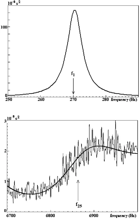
ˆ of the recorded strain in the Nylon bar specimen. _b

Fig. 5. Details of the spectrum

 

ˆ_b2. The thin and thick curves are based on the left and the right member of Eq. (30), respectively. (a) 1st resonance peak, n=1. (b) 25th

(28)

Fig. 6. (a) Phase velocity c and (b) damping coefficient  versus frequency. Open circles: discrete experimental results. Continuous curves: results based on the rheological

model given by Eqs. (12) and (14).

Fig. 7. (a) Real part E and (b) imaginary part E  of the complex modulus E versus frequency. Open circles: discrete experimental results. Filled circles: discrete

noise-corrected results. Continuous curves: results obtained from the rheological model given

by Eqs. (12) and (14).

Fig. 8. Real part E and imaginary part E  of the complex modulus E at low frequencies determined from servo-hydraulic tests.

(29)

Fig. 1. Rheological model with 2



p1



parameters. 0  1  2 p 0  1  2 _p

(30)

Fig. 2. Impact test with a uniform viscoelastic bar specimen.

b a

(31)

Fig. 3. Recorded strain in the Nylon bar specimen. (a) Long-time record of strain pulses

 

t

b

 _{. (b) Primary strain pulse}

 

_t

b

1

followed by strain pulses which have undergone one

(32)

(33)

Fig. 5. Details of the spectrum

 

ˆ_b 2. The thin and thick curves are based on the left and the right member of Eq. (30), respectively. (a) 1st resonance peak, n=1. (b) 25th

(34)

Fig. 6. (a) Phase velocity c and (b) damping coefficient  versus frequency. Open circles: discrete initial results. Continuous curves: results based on the rheological model

(35)

Fig. 7. (a) Real part E and (b) imaginary part E  of the complex modulus E versus frequency. Open circles: discrete initial results. Filled circles: discrete noise-corrected

(36)

Fig. 8. Real part E and imaginary part E  of the complex modulus E at low frequencies determined from servo-hydraulic tests.