Orthotropic strain rate potentials using multiple linear transformations

Science Arts & Métiers (SAM)

is an open access repository that collects the work of Arts et Métiers Institute of Technology researchers and makes it freely available over the web where possible.

This is an author-deposited version published in: https://sam.ensam.eu

Handle ID: .http://hdl.handle.net/10985/9917

To cite this version :

Meziane RABAHALLAH, Tudor BALAN, Frédéric BARLAT - Orthotropic strain rate potentials using multiple linear transformations - International Journal of Solids and Structures - Vol. 46, n°9, p.1966–1974 - 2009

ORTHOTROPIC STRAIN RATE POTENTIALS USING MULTIPLE

LINEAR TRANSFORMATIONS

Meziane Rabahallah*, Tudor Balan*,# Frédéric Barlat** *

LPMM, ENSAM Metz, Arts et Métiers ParisTech, 4 rue A. Fresnel, 57078 Metz Cedex 3, France

**

Materials Mechanics Lab, GIFT, Pohang University of Science and Technology, San 31 Hyoja-dong, Nam-gu, Pohang, Gyeongbuk 790-784, Republic of Korea

ABSTRACT

This paper reviews a class of anisotropic plastic strain-rate potentials, based on linear transformations of the plastic strain-rate tensor. A new formulation is proposed, which includes former models as particular cases and allows for an arbitrary number of linear transformations, involving an increasing number of anisotropy parameters. The formulation is convex and fully three-dimensional, thus being suitable for computer implementation in finite element codes. The parameter identification procedure uses a micromechanical model to generate evenly distributed reference points in the full space of possible loading modes. Material parameters are determined for several anisotropic, fcc and bcc sheet metals, and the gain in accuracy of the new models is demonstrated. For the considered materials, increasing the number of linear transformations leads to a systematic improvement of the accuracy, up to a number of five linear transformations. The proposed model fits very closely the predictions of the micromechanical model in the whole space of plastic strain-rate directions. The r-values, which are not directly used in the identification procedure, served for the validation of the models and to demonstrate their improved accuracy.

KEYWORDS: Anisotropy, Strain rate potentials, Linear transformations, Plasticity, Sheet

metal forming.

#

Corresponding author. E-mail: tudor.balan@ensam.fr (T. Balan); tel: +(33)3.87.37.54.60; fax: +(33)3.87.37.54.70.

1. Introduction

Numerical simulation has become an invaluable tool in sheet metal forming applications and several commercial computer codes are available for this purpose. The accuracy of the simulations directly depends on the ability of the simulation codes to describe the plastic behavior of the material during forming. The description of the initial anisotropy is one of the key factors in improving the reliability of the finite element simulations of forming processes. This is particularly true when final part properties like springback or forming limits are to be predicted.

The plastic anisotropy of sheet metals can be assessed by means of micromechanical

calculations, considering the material as a collection of grains of different orientations, subject to a given loading path and obeying the Schmid law. Nevertheless, the large computing times associated with this method have prevented its wide utilization in an industrial environment. Alternatively, continuum mechanics provide a general theoretical framework for the so-called phenomenological description of plastic anisotropy. This approach is classically based on the use of yield functions ( )φ σ _{and associated flow rules (1) for the computation of stresses and}

strain rates: φ λ ∂ = ′ ∂ ε σ ɺ ɺ (1)

where ′σ _{designates the deviatoric part of the stress tensor} σ_{, εɺ is the plastic strain rate tensor} whileλɺ is the plastic multiplier. However, a potential can be defined either as a function of

stresses (yield criterion) or as a function of strain rates (strain-rate potential). (Ziegler, 1977) and (Hill, 1987) have shown that, based on the plastic work equivalence principle, a

meaningful strain rate potential can be associated with any convex stress potential (or yield surface). The yield criteria act as potential functions for the determination of the plastic strain rate using the flow rule. Equivalently, plastic potentials ( )ψ ε_{ɺ are defined in the space of}

plastic strain-rates and their gradient (2) defines the deviatoric stress (only associated flow rules are considered in the current work, although the theory on hand is not restricted to this particular case): ψ τ ∂ ′ = ∂ σ ε_ɺ (2)

where

τ

is a reference stress (e.g., the yield stress in uniaxial tension along a chosen direction). Formally, the two approaches are identical. For some applications (rigid-plastic FEM simulations (Yoon et al., 1995; Chung et al., 1996; Lee et al., 1997; Ryou et al., 2005), minimum plastic-work path calculations (Chung and Richmond, 1992a; b; 1994; Chung et al., 2000), analytical calculations of simple forming processes etc.) the strain-rate potential

approach can be computationally more suitable. Several fourth order and sixth order strain-rate potentials have been proposed as an adjustment of crystallographic texture functions (Van Houtte et al., 1989; Arminjon and Bacroix, 1991; Arminjon et al., 1994; Savoie and

mathematical function used to define a yield criterion can be transformed in order to describe a plastic potential in the plastic strain-rate space (Barlat and Chung, 1993; Zhou and

Wagoner, 1994).

A useful method to generate both yield criteria and strain-rate potentials is based on the linear transformation of the stress tensor or the plastic strain-rate tensor, respectively. Yield

functions using the linear transformation of the stress tensor were proposed in the early 90s by (Barlat et al., 1991) and (Karafillis and Boyce, 1993). In an attempt to increase the number of parameters, two independent linear transformations have been used in the formulation of the plane stress potential Yld2000-2d (Barlat et al., 2000; Barlat et al., 2003). Full 3D yield functions employing two linear transformations have been proposed by (Barlat et al., 2005) and (Bron and Besson, 2004) – the later also proposed a generic form of yield function as a sum of several functions.

In parallel, the strain rate potential Srp93 (Barlat and Chung, 1993; Barlat et al., 1993), which is the pseudo-conjugate of the Yld91 stress potential (Barlat et al., 1991), was developed using a linear transformation of the plastic strain rate tensor. The strain rate potential

Srp2003-2d, which is the pseudo-conjugate of the Yld2000-2d stress potential (Barlat et al., 2003), was proposed by (Kim et al., 2003a) subsequently. Recently, (Barlat and Chung, 2005; Kim et al., 2007) proposed the two-transformation strain-rate potentials Srp2004-18p and Srp2006-18p, inspired from the expression of the yield criterion Yld2004-18p (Barlat et al., 2005).

The increased flexibility of these potentials allowed both the uniaxial yield stresses and the corresponding r-values to be taken into account simultaneously for parameter identification. The later versions describe accurately such uniaxial tensile test results performed every 15°. Finite element simulation of springback as well as forming limit predictions have been performed by (Kim et al., 2003b; Chung et al., 2005) with Yld2000-2d and by (Li et al., 2003) and (Hiwatashi et al., 1998) with the sixth order potential developed by (Van Houtte et

al., 1989) with very good results. Also, the number, position and relative height of the ears in cylindrical cup drawing are better predicted with recent yield criteria (see e.g. (Yoon et al., 2006)). In particular, (Rabahallah et al., 2006; Rabahallah et al., 2008a) have shown that the Srp2004-18p potential predicts the initial anisotropy better than most of the existing

phenomenological potentials for a very wide range of materials. This is a potentially interesting property since a unique mathematical function could be used for all the forming applications, while some former mathematical functions were known to perform better e.g. for either bcc or fcc sheet materials, but nor for both (Bacroix et al., 2003).

The aim of this paper is to explore more systematically the use of linear transformations in the formulation of plastic strain-rate potentials. In section 2, a general formulation is proposed involving an arbitrary number of linear transformations. This formulation includes former plastic strain-rate potentials as particular cases. The number of parameters is increasing with the number of linear transformations; their identification is tackled in section 3 for a number of sheet metals – both bcc and fcc. Section 4 shows the ability of the different models to accurately predict the yield surface, the curves of plastic potential iso-values as well as the r-values for the selected materials. The mathematical details for the complete calculation of the plastic potential and its derivatives are given in appendix.

2. Formulation of the proposed model

As mentioned in the introduction, linear transformation of the stress tensor σ _{by means of an} anisotropic operator B provides a straightforward way to generalize isotropic yield functions to anisotropy (Barlat et al., 1991; Karafillis and Boyce, 1993; Barlat et al., 2005). The same technique can be applied to the plastic strain-rate tensor εɺ in order to generalize isotropic expressions of plastic potentials. The following linear transformation has been used by (Barlat and Chung, 2005; Kim et al., 2007), which enforces the deviatoric character of the plastic strain-rate tensor in a convenient way:

= ⋅ ⋅

εɶɺ _{B T εɺ (3)}

In Eq. (3), T designates the unit tensor in the space of fourth order symmetric deviatoric tensors while the fourth order array B contains anisotropy coefficients. For the case of orthotropic symmetry, these tensors can be represented as the following 6×6 arrays:

12 13 21 23 31 32 44 55 66 0 0 0 0 0 0 0 0 0 0 0 0 0 0 0 0 0 0 0 0 0 0 0 0 0 0 0 b b b b b b b b b − −     − −   _{− −}  =            B ; 2 1 1 _{0 0 0} 3 3 3 1 2 1 _{0 0 0} 3 3 3 1 1 2 _{0 0 0} 3 3 3 0 0 0 1 0 0 0 0 0 0 1 0 0 0 0 0 0 1 − −     _{− −}    _{− −}  =             T (4)

In order to use these compact notations, the εɺ -like tensors are written here as 6-component vectors; e.g., ε_ɺ=[

ε

_ɺxx

ε

_ɺyy

ε

_ɺzz

ε

_ɺyz

ε

_ɺzx

ε

_ɺxy]T_{, with components in the frame of material}

symmetry.

The following scalar functions are used in defining the strain-rate potentials Srp93, Srp2004-18p and Srp2006-Srp2004-18p:

(

)

(

)

1 1 2 3 2 2 3 3 1 1 2 , , b b b b b b E E E E E E E E E = + + = + + + + + B ε B ε ϕ ϕ ɶ ɶ ɶ ɺ ɶ ɶ ɶ ɶ ɶ ɶ ɺ (5)

where Eɶ_i are the principal values of tensor εɶɺ defined by the linear transformation of Eq. (3). The notations in Eq. (5) allow rewriting the existing members of the Srp-family of strain-rate potentials in the following compact forms:

( )

(

)

( )

(

)

(

)

( )

(

)

(

)

1 1 1 1 1 2 1 2 2 1 1 2 1 1 2 1 (a) Srp93: , 2 1 1 (b) Srp2004-18p: , , 2 2 1 (c) Srp2006-18p: , , 2 2 b b b b b b − − −   =  = +    _{ } = _ + _ = +    _{ } = _ + _ = +   ε _{B ε} ε _{B ε B ε} ε _{B ε B ε}

ψ

ϕ

ε

ψ

ϕ

ϕ

ε

ψ

ϕ

ϕ

ε

ɺ ɺ ɺ ɺ ɺ ɺ ɺ ɺ ɺ ɺ ɺ (6)

where εɺ is the effective plastic strain rate, which is the conjugate of the effective stress σ

under the plastic work rate equivalence principle.

Eqs. (6)b and (6)c represent two different extensions of Eq. (6)a, each of them using two linear transformations. The Srp2006-18p expression uses function

ϕ

₁ twice, which may rise uniqueness problems during parameter identification. In (Kim et al., 2007), Srp2004-18p and Srp2006-18p have shown almost identical predictions and convergence behavior. Therefore, any of them could be used to further increase the number of linear transformations in the plastic potential expressions. In this perspective, Srp2006-18p has the advantage of a unique definition for odd number of transformations and to yield the most compact formula for a multiple transformation potential.

In this work, the following generalization is proposed, using multiple linear transformations of the plastic strain-rate tensor:

( )

(

)

1 1 1 1 1 1 , 2 1 N _b k b k N

ψ

₋

ϕ

ε

=   =  = + 

∑

 ε_{ɺ B εɺ} ɺ ₍₇₎

The expressions of Srp931 and Srp2006-18p are particular cases of the function proposed above, for N=1 and N=2. Larger N-values lead to new expressions, involving an increased mathematical flexibility – associated with an increased number of parameters. All these expressions can be designated as Srp2007-N×9p potentials.

The strain rate potentials

ψ

are proven to be convex (Rockafellar, 1970) in the space of the principal transformed strain rates Eɶ_i (note the sum of two or more convex functions is also a convex function) and it is easy to show that they are also convex with respect to the plastic strain rate tensor (Kim et al., 2007). Thus, the series of potentiels generated with Eq. (7) are convex functions.

3. Parameter identification

1

The original expression of Srp93 (Barlat and Chung, 1993) is slightly different since a simpler anisotropy matrix has been used at that time (involving seven parameters, instead of nine). However, the current equation can be considered as the final version of Srp93.

Successful parameter identification is a key problem for the advanced potentials involving an increasing number of parameters. Moreover, the need for specific experimental measures that often differ from one model to another makes it almost impossible to consistently compare the predictions of different models.

It has been recently shown by (Plunkett et al., 2008) that the identification of yield functions based on multiple linear transformations can be performed using experimental data obtained by mechanical tests. However, a more consistent approach for model comparison is provided by the texture-based identification introduced in the early 90s by (Van Houtte et al., 1989; Arminjon and Bacroix, 1991). In this case, a very large number of reference points is generated by means of a micromechanical model. These points are evenly distributed in the space of plastic strain-rate directions. For this purpose, the plastic strain-rate directions

=

N ε ε_{ɺ ɺ are represented by five-component unit vectors (Lequeu et al., 1987), as described} in appendix. Such unit vectors can be described in the 5D space by four angles

1, 2, 3 and 4

θ θ θ

θ

(Gilormini et al., 1988): 1 1 2 3 4 2 1 2 3 4 3 2 3 4 4 3 4 5 4

cos sin sin sin sin sin sin sin cos sin sin cos sin cos N N N N N

θ

θ

θ

θ

θ

θ

θ

θ

θ

θ

θ

θ

θ

θ

= = = = = (8)

where 0≤

θ

1≤2π and 0≤

θ

i≤π, for i between 2 and 4. Consequently, the element of area on the

unit hypersphere defined in this way equals

(

)

₍

2

₎

1 cos 2 3 2 sin 2 3 4 2 sin 4 cos 4 3

d dθ θ d θ − θ d _ + θ θ _{ . The orthotropic symmetry of the} texture of rolled materials allows for a reduction of the range of each of the four angles as follows (Arminjon and Bacroix, 1991): 0≤

θ

1≤2π; -1≤cos

θ

2≤1; 0≤θ3 2 sin 2− θ3 4≤π/4;

0≤

(

2

)

4 4

2 sin+ θ cosθ 3≤2/3. These variation ranges are swept with regular intervals, yielding a discretisation of 40 20 10 10× × × points, which correspond to unit vectors in the space of plastic strain-rates. Consequently, the number of reference points for the identification (80,000) is much larger than the number of parameters of the models. Moreover, this approach allows one to investigate the models’ ability to describe the through-thickness anisotropy of the materials. Indeed, this type of anisotropic response is difficult (and most often impossible) to address by means of experimental testing. While most sheet metals are strained in the plane of the sheet during forming, several applications (e.g. multi-pass forming, thick sheet forming, hemming etc.) may involve non-negligible through-thickness shear strains.

A rigid-plastic, “full-constraints” Taylor model (Bishop and Hill, 1951) is used to generate the reference values used for the identification procedure. The families of slip systems considered are

{ }

111 110 for fcc metals and

{

110 111

}

,

{

112 111

}

for bcc metals. The same critical resolved shear stress was considered on all slip systems; its value is not relevant for the current analysis since the calculated stresses are normalized by the resolved shear stress throughout. Hardening modeling is also not required, nor texture evolution, since only the initial yielding point is calculated. It is noteworthy that any other micromechanical model

can be used to generate these reference yielding points for the parameter identification. Given a unit plastic strain rate tensor N , the corresponding average plastic work rate Wɺ_TaylorP

( )

N and the normalized expression _TaylorP

( )

:

c

τ

′

Π N =σ N can be computed, where

τ

cis the critical shear

stress associated with the Schmid law on the crystallographic slip systems. The same

quantities can be calculated by using the plastic potential. Since the different potentials used in this work are described by homogeneous function of degree one, Eq. (7) can be rewritten in terms of N, as

( )

( )

P W

ψ

τ

= N N ɺ (9)

where

τ

is the reference stress for the plastic potentials. In other words, for any strain rate direction N , the previously defined two functions _i ΠTaylorP

( )

Ni and

ψ

( )

Ni correspond to the

plastic work rate associated with a unit-norm strain rate tensor and normalized by the reference stress. The coefficients of the plastic potential

ψ

can then be identified by minimizing the following objective function:

( )

( )

( )

80000 ₂ 1 80000 ₂ 1 (material parameters) P Taylor i i i P Taylor i i F

ψ

= = _{Π −}    = _Π   

∑

∑

N N N (10)

with respect to the parameters of the chosen potential. The sum is performed over the 80,000 predefined strain rate directions discussed earlier. The values Π_TaylorP

( )

N_i are computed for all these directions. This is a lengthy task, but it has to be performed only once for each material. In the recent papers (Rabahallah et al., 2008a; Van Houtte et al., 2008), such procedures have been used for the parameter identification of various plastic strain-rate potentials and are described in detail.

4. Application to steel and aluminum alloy sheet metals

4.1 Materials and material parameters

The experimental textures of a set of six polycrystalline materials have been used for the current investigation: three aluminum alloy sheets and three steel sheets. The three aluminum alloy sheets are an aluminum-magnesium-silicium alloy AA6016, an aluminum-magnesium aluminum alloy AA5182 and an AA6022 alloy. The steel sheets are an interstitial free mild steel DC06, a high stength Dual phase steel DP600 and a high strength low-alloyed steel HSLA340. All these materials are widely used in the automotive industry and have been thoroughly investigated in (3DS, 2001; Haddadi et al., 2006). The microstructure of the steel sheets has been investigated in (Nesterova et al., 2001; Gardey et al., 2005a; Gardey et al., 2005b).

Figure 1 shows the yield surfaces and the in-plane variation of Hill’s anisotropy coefficient

2 1

r= ε εɺ ɺ for the six materials under investigation, as predicted by the crystal plasticity model. The two high strength steels DP600 and HSLA are almost isotropic and their yield surfaces are very close to each other. The three aluminum alloy sheets exhibit r-values smaller than one, with a strong variation for AA6022. In contrast, the mild steel exhibits an average r-value of two, with an in-plane variation close to unity. The experimental r-r-values for all these materials as well as the predictions of several existing plastic potentials are available in (Rabahallah et al., 2008a).

The values of the material parameters identified for these materials and for the Srp2007 model for up to six transformations are given in Tables 1 to 4. In the next section, these results are analyzed in terms of yield surface plots, strain-rate potential iso-values plots, r-value plots and parameter identification objective function values.

-4 -3 -2 -1 0 1 2 3 4 -4 -3 -2 -1 0 1 2 3 4 DP600 HSLA AA6022 AA5182 AA6016 DC06 0.0 0.5 1.0 1.5 2.0 2.5 3.0 0 10 20 30 40 50 60 70 80 90 DC06 HSLA DP600 AA5182 AA6016 AA6022 xx c

σ

τ

yy c

σ

τ

Figure 1. Yield surfaces (top) and r-values (bottom) for the six materials of the study; Taylor model predictions.

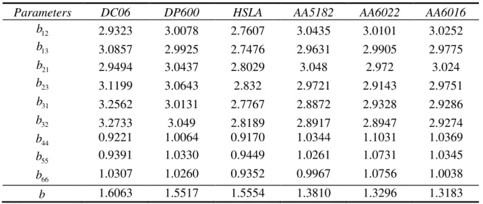
Table 1. Best fit parameters of the Srp2007-1×9p after identification, for the six materials.

Parameters DC06 DP600 HSLA AA5182 AA6022 AA6016

12 b _{2.9323 3.0078 2.7607 3.0435 3.0101 3.0252} 13 b _{3.0857 2.9925 2.7476 2.9631 2.9905 2.9775} 21 b _{2.9494 3.0437 2.8029 3.048 2.972 3.024} 23 b _{3.1199 3.0643 2.832 2.9721 2.9143 2.9751} 31 b _{3.2562 3.0131 2.7767 2.8872 2.9328 2.9286} 32 b _{3.2733 3.049 2.8189 2.8917 2.8947 2.9274} 44 b 0.9221 1.0064 0.9170 1.0344 1.1031 1.0369 55 b 0.9391 1.0330 0.9449 1.0261 1.0731 1.0345 66 b 1.0307 1.0260 0.9352 0.9967 1.0756 1.0038 b 1.6063 1.5517 1.5554 1.3810 1.3296 1.3183

Table 2. Best fit parameters of the Srp2007-2×9p after identification, for the six materials.

Parameters DC06 DP600 HSLA AA5182 AA6022 AA6016

1 12 b _{0.9552 0.1341 0.6176 1.5420 0.3174 1.6189} 1 13 b _{0.9893 0.5141 0.3453 1.5109 0.0152 1.5707} 1 21 b _{1.2842 1.1634 0.0739 1.6337 0.7568 1.5482} 1 23 b _{1.2377 1.0563 0.2236 1.6230 0.2410 1.5707} 1 31 b _{1.2117 0.6356 -0.1288 1.5248 0.4022 1.5328} 1 32 b _{1.2144 0.5963 0.2200 1.5096 0.2673 1.6076} 1 44 b _{1.3448 0.7458 0.4057 1.6772 0.7076 1.5492} 1 55 b _{1.1439 -0.0087 0.4666 1.5940 0.4440 1.7014} 1 66 b _{1.3870 0.5735 0.5414 1.6138 0.1820 1.5902} 2 12 b _{0.5695 1.1936 1.2852 0.2844 1.3642 0.3379} 2 13 b _{-0.4002 1.3097 1.3884 0.2877 1.4038 0.2762} 2 21 b _{0.6464 1.2247 1.2628 0.3904 1.4569 0.0606} 2 23 b _{-0.2051 1.1146 1.3572 0.2079 1.4284 0.1440} 2 31 b _{-0.1529 1.3339 1.3789 0.3413 1.5882 0.2327} 2 32 b _{-0.7111 1.0895 1.4639 0.2916 1.5605 0.1851} 2 44 b _{-0.4046 1.1794 1.3121 -0.0985 1.4803 0.4216} 2 55 b _{-0.8189 1.5432 1.3321 0.2969 1.6225 0.1171} 2 66 b _{0.5119 1.3890 1.2562 0.2574 1.7888 0.2447} b 1.4990 1.5171 1.5000 1.2878 1.2640 1.3333

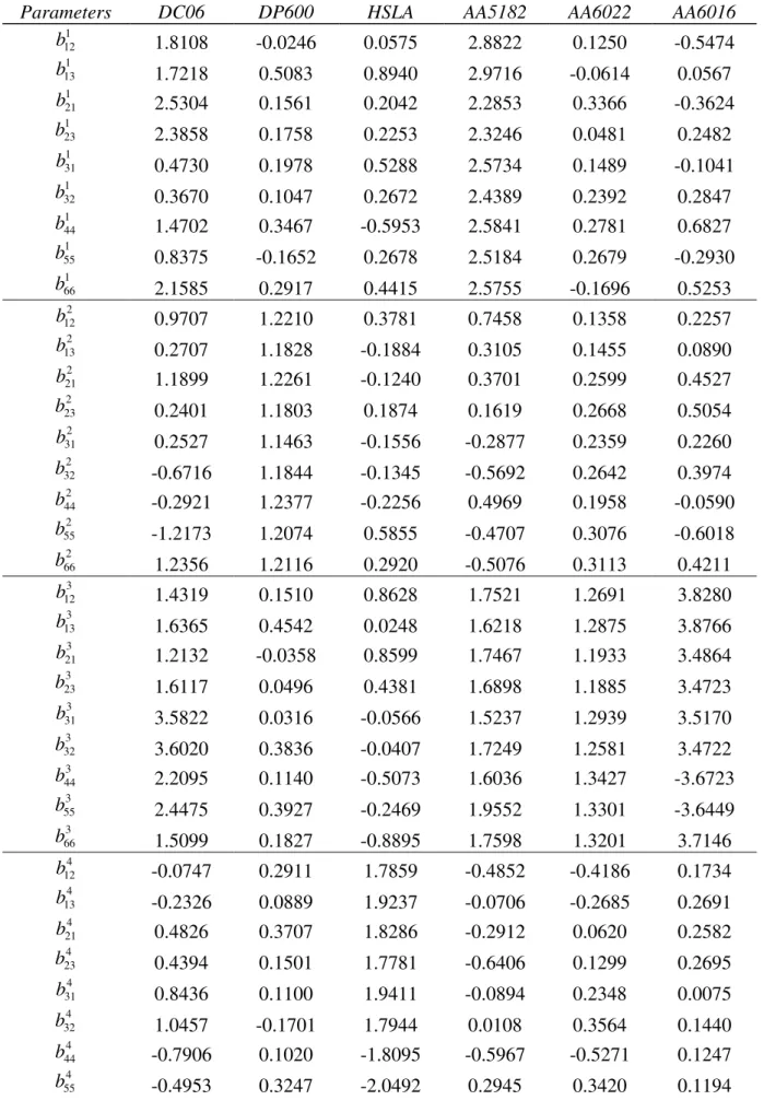
Table 3. Best fit parameters of the Srp2007-4×9p after identification, for the six materials.

Parameters DC06 DP600 HSLA AA5182 AA6022 AA6016

1 12 b _{1.8108 -0.0246 0.0575 2.8822 0.1250 -0.5474} 1 13 b _{1.7218 0.5083 0.8940 2.9716 -0.0614 0.0567} 1 21 b 2.5304 0.1561 0.2042 2.2853 0.3366 -0.3624 1 23 b _{2.3858 0.1758 0.2253 2.3246 0.0481 0.2482} 1 31 b _{0.4730 0.1978 0.5288 2.5734 0.1489 -0.1041} 1 32 b _{0.3670 0.1047 0.2672 2.4389 0.2392 0.2847} 1 44 b _{1.4702 0.3467 -0.5953 2.5841 0.2781 0.6827} 1 55 b _{0.8375 -0.1652 0.2678 2.5184 0.2679 -0.2930} 1 66 b _{2.1585 0.2917 0.4415 2.5755 -0.1696 0.5253} 2 12 b _{0.9707 1.2210 0.3781 0.7458 0.1358 0.2257} 2 13 b _{0.2707 1.1828 -0.1884 0.3105 0.1455 0.0890} 2 21 b _{1.1899 1.2261 -0.1240 0.3701 0.2599 0.4527} 2 23 b _{0.2401 1.1803 0.1874 0.1619 0.2668 0.5054} 2 31 b _{0.2527 1.1463 -0.1556 -0.2877 0.2359 0.2260} 2 32 b _{-0.6716 1.1844 -0.1345 -0.5692 0.2642 0.3974} 2 44 b _{-0.2921 1.2377 -0.2256 0.4969 0.1958 -0.0590} 2 55 b _{-1.2173 1.2074 0.5855 -0.4707 0.3076 -0.6018} 2 66 b _{1.2356 1.2116 0.2920 -0.5076 0.3113 0.4211} 3 12 b 1.4319 0.1510 0.8628 1.7521 1.2691 3.8280 3 13 b _{1.6365 0.4542 0.0248 1.6218 1.2875 3.8766} 3 21 b _{1.2132 -0.0358 0.8599 1.7467 1.1933 3.4864} 3 23 b _{1.6117 0.0496 0.4381 1.6898 1.1885 3.4723} 3 31 b _{3.5822 0.0316 -0.0566 1.5237 1.2939 3.5170} 3 32 b _{3.6020 0.3836 -0.0407 1.7249 1.2581 3.4722} 3 44 b 2.2095 0.1140 -0.5073 1.6036 1.3427 -3.6723 3 55 b _{2.4475 0.3927 -0.2469 1.9552 1.3301 -3.6449} 3 66 b _{1.5099 0.1827 -0.8895 1.7598 1.3201 3.7146} 4 12 b _{-0.0747 0.2911 1.7859 -0.4852 -0.4186 0.1734} 4 13 b _{-0.2326 0.0889 1.9237 -0.0706 -0.2685 0.2691} 4 21 b _{0.4826 0.3707 1.8286 -0.2912 0.0620 0.2582} 4 23 b _{0.4394 0.1501 1.7781 -0.6406 0.1299 0.2695} 4 31 b _{0.8436 0.1100 1.9411 -0.0894 0.2348 0.0075} 4 32 b _{1.0457 -0.1701 1.7944 0.0108 0.3564 0.1440} 4 44 b _{-0.7906 0.1020 -1.8095 -0.5967 -0.5271 0.1247} 4 55 b _{-0.4953 0.3247 -2.0492 0.2945 0.3420 0.1194}

4 66

b _{0.7161 0.4254 1.8071 0.4361 0.4300 0.0854} b 1.4537 1.4444 1.4580 1.2733 1.1970 1.2884

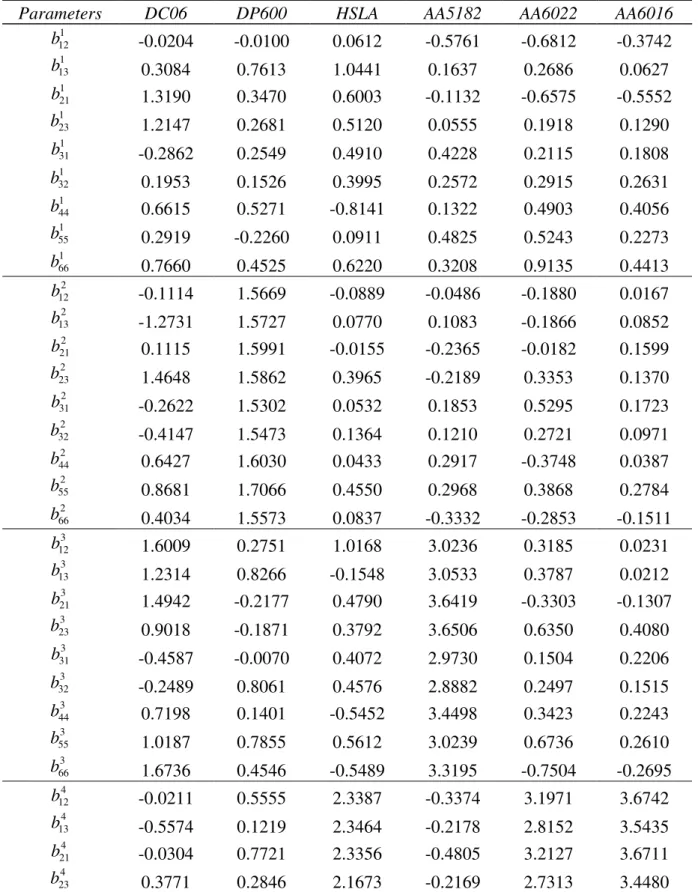
Table 4. Best fit parameters of the Srp2007-6×9p after identification, for the six materials.

Parameters DC06 DP600 HSLA AA5182 AA6022 AA6016

1 12 b _{-0.0204 -0.0100 0.0612 -0.5761 -0.6812 -0.3742} 1 13 b _{0.3084 0.7613 1.0441 0.1637 0.2686 0.0627} 1 21 b _{1.3190 0.3470 0.6003 -0.1132 -0.6575 -0.5552} 1 23 b _{1.2147 0.2681 0.5120 0.0555 0.1918 0.1290} 1 31 b _{-0.2862 0.2549 0.4910 0.4228 0.2115 0.1808} 1 32 b _{0.1953 0.1526 0.3995 0.2572 0.2915 0.2631} 1 44 b 0.6615 0.5271 -0.8141 0.1322 0.4903 0.4056 1 55 b _{0.2919 -0.2260 0.0911 0.4825 0.5243 0.2273} 1 66 b _{0.7660 0.4525 0.6220 0.3208 0.9135 0.4413} 2 12 b _{-0.1114 1.5669 -0.0889 -0.0486 -0.1880 0.0167} 2 13 b _{-1.2731 1.5727 0.0770 0.1083 -0.1866 0.0852} 2 21 b _{0.1115 1.5991 -0.0155 -0.2365 -0.0182 0.1599} 2 23 b _{1.4648 1.5862 0.3965 -0.2189 0.3353 0.1370} 2 31 b _{-0.2622 1.5302 0.0532 0.1853 0.5295 0.1723} 2 32 b _{-0.4147 1.5473 0.1364 0.1210 0.2721 0.0971} 2 44 b _{0.6427 1.6030 0.0433 0.2917 -0.3748 0.0387} 2 55 b _{0.8681 1.7066 0.4550 0.2968 0.3868 0.2784} 2 66 b _{0.4034 1.5573 0.0837 -0.3332 -0.2853 -0.1511} 3 12 b _{1.6009 0.2751 1.0168 3.0236 0.3185 0.0231} 3 13 b _{1.2314 0.8266 -0.1548 3.0533 0.3787 0.0212} 3 21 b 1.4942 -0.2177 0.4790 3.6419 -0.3303 -0.1307 3 23 b _{0.9018 -0.1871 0.3792 3.6506 0.6350 0.4080} 3 31 b _{-0.4587 -0.0070 0.4072 2.9730 0.1504 0.2206} 3 32 b _{-0.2489 0.8061 0.4576 2.8882 0.2497 0.1515} 3 44 b _{0.7198 0.1401 -0.5452 3.4498 0.3423 0.2243} 3 55 b _{1.0187 0.7855 0.5612 3.0239 0.6736 0.2610} 3 66 b _{1.6736 0.4546 -0.5489 3.3195 -0.7504 -0.2695} 4 12 b _{-0.0211 0.5555 2.3387 -0.3374 3.1971 3.6742} 4 13 b _{-0.5574 0.1219 2.3464 -0.2178 2.8152 3.5435} 4 21 b _{-0.0304 0.7721 2.3356 -0.4805 3.2127 3.6711} 4 23 b _{0.3771 0.2846 2.1673 -0.2169 2.7313 3.4480}

4 31 b _{0.5515 0.1519 2.3421 0.5421 2.7563 3.4962} 4 32 b _{0.4170 -0.3576 2.1801 0.0985 2.6202 3.4384} 4 44 b _{0.5728 0.2566 -2.2694 -0.4211 2.8726 3.5866} 4 55 b _{0.0963 0.6901 -2.4028 0.2874 2.9857 3.5437} 4 66 b _{0.5917 0.8071 2.3531 0.4052 3.1534 3.6237} 5 12 b _{1.7587 0.0345 0.4517 0.6316 0.3407 0.5819} 5 13 b _{1.7506 0.7790 0.9307 0.5767 -0.4496 -0.1231} 5 21 b _{1.5999 0.2817 0.2540 0.5757 0.3839 0.2740} 5 23 b _{1.6588 0.1927 0.1037 0.5036 0.4709 0.1226} 5 31 b _{1.8413 0.2452 -0.0447 0.8257 0.3340 0.3014} 5 32 b _{1.7790 0.1044 0.3951 0.9680 0.2198 0.1211} 5 44 b _{1.9096 0.5467 0.5048 0.6466 0.6754 0.5542} 5 55 b _{1.8587 -0.2277 0.7055 -0.9417 0.5226 0.2993} 5 66 b _{1.7113 0.4612 0.6013 -0.6798 0.7848 0.4293} 6 12 b 0.2847 1.6012 -0.5906 0.4099 -0.5784 -0.0464 6 13 b _{-0.4844 1.5164 -0.2412 0.6187 -0.7969 -0.2476} 6 21 b _{0.2817 1.6132 -0.6961 0.5359 0.6842 0.2714} 6 23 b _{-0.0092 1.5295 -0.3278 0.0597 0.7985 0.3726} 6 31 b _{-0.0525 1.5291 -0.2991 -0.1592 -0.2348 0.0113} 6 32 b _{-0.3292 1.5643 0.3036 0.0322 0.3294 0.1837} 6 44 b _{-0.3845 1.5876 -0.1323 0.2219 1.1082 0.1047} 6 55 b _{0.8323 1.5116 0.7546 0.4050 0.5963 0.4537} 6 66 b _{0.2364 1.5918 0.7783 0.3244 -0.3460 -0.2862} b 1.3547 1.4685 1.4382 1.2555 1.1530 1.2624

4.2 Analysis of results and discussion

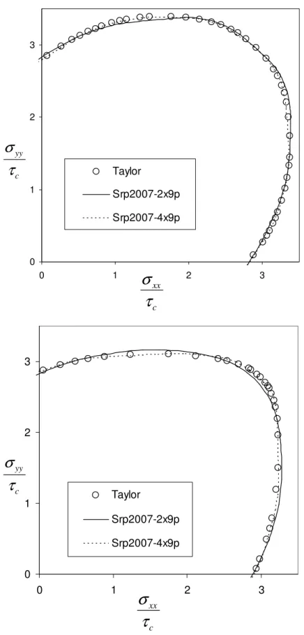
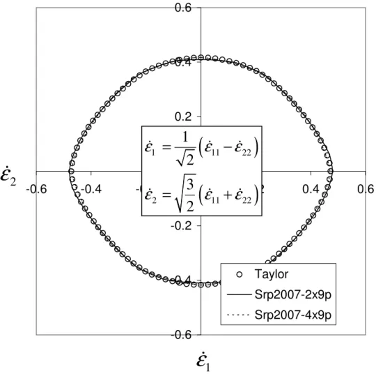
Figure 2 displays the yield surface for the AA6022 aluminum alloy as well as the DC06 mild steel, as predicted by Srp2007-2×9p and Srp2007-4×9p. Figure 3 displays the deviatoric plane of the corresponding dual equipotential surfaces for the mild steel. One can see that Srp2007-4x9p almost perfectly fits the reference points corresponding to the micromechanical model. However, the prediction provided by Srp2007-2×9p is already very close to this reference. A more quantitative comparison can be made by considering the values of the objective-function (10) as a measure of the closeness of each model to the reference data. Figure 4 summarizes the values of the objective functions for the Srp2007 models for up to six linear

0 1 2 3 0 1 2 3 Taylor Srp2007-2x9p Srp2007-4x9p xx c

σ

τ

yy c

σ

τ

0 1 2 3 0 1 2 3 Taylor Srp2007-2x9p Srp2007-4x9p xx c

σ

τ

yy c

σ

τ

Figure 2. Normal plane stress yield surface for a DC06 mild steel (top) and an AA6022 aluminum alloy (bottom).

-0.6 -0.4 -0.2 0.0 0.2 0.4 0.6 -0.6 -0.4 -0.2 0.0 0.2 0.4 0.6 Taylor Srp2007-2x9p Srp2007-4x9p

(

)

(

)

1 11 22 2 11 22

1

2

3

2

=

−

=

+

ɺ

ɺ

ɺ

ɺ

ɺ

ɺ

ε

ε

ε

ε

ε

ε

1

ɺ

ε

2

ɺ

ε

Figure 3.

π

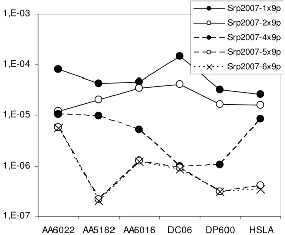
-plane plot of plastic strain-rate potentials for the mild steel DC06.

Figure 4 gives a global picture of the respective ability of the various models to describe the plastic anisotropy of sheet metals. It appears clearly that considering up to four or five linear transformation in the Srp2007 expression allows for an improvement in accuracy and

flexibility. However, the addition of the sixth transformation brings almost no improvement for all the materials and it appears useless to increase complexity beyond this value.

1,E-07 1,E-06 1,E-05 1,E-04 1,E-03

AA6022 AA5182 AA6016 DC06 DP600 HSLA

Srp2007-1x9p Srp2007-2x9p Srp2007-4x9p Srp2007-5x9p Srp2007-6x9p

Figure 4. Values of the minimum objective function after parameter identification of different versions of the Srp2007 model, for each of the six materials.

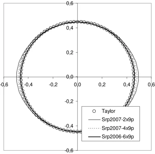
While these conclusions are clearly reproduced for all the materials in this study, it is not obvious from Figure 2 and Figure 3 that a significant improvement has been obtained in the shape of the yield locus, e.g. when four linear transformations are used instead of only two for the DC06 mild steel sheet. Figure 5 provides a different graphical representation of the five-dimensional equipotential surface predicted for the DC06 mild steel: a two-five-dimensional cut is made in this surface through a plane containing the two through-thickness shear components2. It appears clearly from this graph that the use of more than two linear transformations

improves the predictions in the whole five-dimensional space of possible plastic strain-rate directions, which explains the diminution of the corresponding error function by more than one order of magnitude.

2

The variables on the two axes are scaled in such a way that a von Mises model would be represented by circles in all these graphs. More details about this scaling are given in appendix.

-0,6 -0,4 -0,2 0,0 0,2 0,4 0,6 -0,6 -0,4 -0,2 0,0 0,2 0,4 0,6 Taylor Srp2007-2x9p Srp2007-4x9p Srp2006-6x9p

Figure 5. Scaled εɺ_xz−εɺ plot of plastic strain-rate potentials for the mild steel DC06. _yz

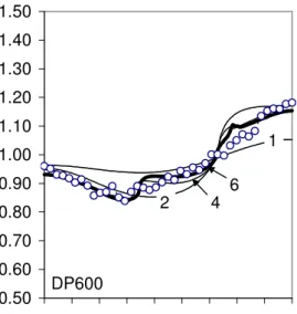
In contrast to the regular parameter identification method that uses mechanical test data, it is noteworthy here that the r-values have not been used for the identification. Consequently, they can be used as a means of validation. Figure 6 depicts the predictions of the r-values for all the materials analyzed in this work, as predicted by the Taylor model and by the Srp2007 models with up to six transformations. First, let us note that the Taylor model is known to predict the anisotropy coefficients rather poorly; this prevents the use of this data for the parameter identification. Moreover, the crystal plasticity predictions in Figure 6 are slightly noisy. From this figure and from Figure 1b, it is obvious that for the aluminum alloys, for which only one slip system is used, the r-value variation smoothly oscillates with a period of 10°. This corresponds to the step of discretization of the Euler angles when the orientation distribution function is constructed for each material (2016 crystallographic orientations are used to describe the orientation distribution function).

Nevertheless, it is obvious from these graphs that additional linear transformations in the Srp2007 model improve the prediction of the r-values for most materials. The predictions of the two-transformation model consistently improve the predictions with respect to the one-transformation one; yet they are still inaccurate for some materials. However, for all the materials investigated, the four-transformation and six-transformation versions laid very close to the micromechanical model predictions – remaining in the error range of the Taylor model itself. On the other side, the increased flexibility of the multiple-transformation potential

sometimes led to numerous oscillations of the anisotropy coefficient in the neighborhood the reference curve. Mathematically speaking, these oscillations lay close to the reference data and most of the time they are smaller than the error range of the Taylor model; thus no better result could be expected from the automatic identification procedure. However, the

smoothness of the r-value in-plane variation is a pre-requisite for a correct prediction e.g. of the cup drawing ears – more generally the flow anisotropy prediction in finite element simulations (Rabahallah et al., 2008b). As a consequence, the robust parameter identification of the Srp2007 models might require a smoothing procedure in order to enforce the realistic variation of the anisotropy coefficient.

These results also show that, especially for the more usual potentials (i.e. with one or two transformations), excluding the r-values from the reference data used for identification may lead to inaccurate results. This observation is well known in the case when a reduced number of experimental data are used for the identification. Here, the same conclusion is obtained even if the number of stress points is very large and evenly distributed in the whole space of possible loading directions.

Due to the restricted range of application of the Taylor model, the use of the current

identification technique cannot eliminate completely the experimental results without loss of accuracy. Instead, it provides a consistent method to compare plasticity models and it also allows, in combination with experimental results, for a better identification of the potential parameters affecting the through-thickness shear terms, which cannot be identified by means of experimental data only.

1.00 1.20 1.40 1.60 1.80 2.00 2.20 2.40 2.60 2.80 0 10 20 30 40 50 60 70 80 90 1 2 4 6 DC06 0.20 0.30 0.40 0.50 0.60 0.70 0.80 0.90 1.00 1.10 1.20 0 10 20 30 40 50 60 70 80 90 1 2 4 6 AA5182 0.20 0.30 0.40 0.50 0.60 0.70 0.80 0.90 1.00 1.10 1.20 0 10 20 30 40 50 60 70 80 90 1 2 4 6 AA6022 0.20 0.30 0.40 0.50 0.60 0.70 0.80 0.90 1.00 1.10 1.20 0 10 20 30 40 50 60 70 80 90 1 2 4 6 AA6016 0.50 0.60 0.70 0.80 0.90 1.00 1.10 1.20 1.30 1.40 1.50 0 10 20 30 40 50 60 70 80 90 1 2 4 6 DP600 0.50 0.60 0.70 0.80 0.90 1.00 1.10 1.20 1.30 1.40 1.50 0 10 20 30 40 50 60 70 80 90 1 2 4 6 HSLA

Figure 6. Predictions of the in-plane variation of r-values for the six materials studied in the paper. The reference data (r-values predicted with the Taylor model – represented by open circles) have not been used for the parameter identification. The numbers on the plots (1, 2, 4

and 6) designate the number of transformations (the thick lines designate the six-transformation potential).

5. Conclusions

A new formulation of plastic strain-rate potentials has been proposed that includes as

particular cases the previous members of the Srp-family of plastic potentials. This expression allows for arbitrarily increasing the number of parameters. It has been shown that each additional linear transformation corresponds to a clear improvement in the flexibility of the obtained model, for a wide range of steel and aluminum alloy sheets, up to five

transformations.

The use of the texture-based identification approach has shown that the through-thickness predictions of the Srp-models are also improving when additional linear transformations are used. The four-transformation version almost perfectly reproduces the micromechanical model for the particular materials studied in this work. This, as well as the use of a large set of evenly-distributed reference points, is a major advantage of the texture-based identification approach.

In practice, this parameter identification technique is restricted to sheet metals where the considered micromechanical model is known to correctly describe the real plastic anisotropy of the material. In this case, this approach not only generates accurate parameters, but it does so at a much lower cost as compared to the experimental method. For most practical

applications, however, experimental data (r-values, uniaxial and biaxial yield stresses etc.) shall be used for the identification; if necessary, micromechanical calculations can be added (with a reduced weight in the objective function) to the experimental data set in order to identify all the parameters of the potential (Kim et al., 2007).

Future work concerns the generalization of this approach to the Yld-family of yield criteria – as it has already been applied e.g. by (Plunkett et al., 2008) for the CB2006 criterion.

Acknowledgements

The authors are grateful to Brigitte Bacroix and Salima Bouvier for providing the Taylor model code and the experimental texture data, and for fruitful discussions. The first author is grateful to the Région Lorraine, France, for its three-year financial support.

Appendix 1: Strain rate potential first derivatives

(

)

1 1 1 1 1 2 1 k b N k b k N b − − =  _{∂ ∂}  ∂ =  ⋅  ∂ +

∑

∂ ∂  E ε _E ε ɶ ɶ ɺ ɺ

ϕ

ψ

ψ

(11)

For the general expression of Srp2007-N×9p shown in Eq. (7), the expressions for

1 , 1,3 k i E i

ϕ

∂ ∂ɶ = are 2 1 k k b i i k i bE E E

ϕ

− ∂ = ∂ɶ ɶ ɶ (12)

The terms ∂Eɶk ∂ε_{ɺ are independent of the number of transformations in the potential and their}

calculation is provided in (Kim et al., 2007).

Appendix 2: Five-component notation for symmetric deviatoric

tensors

Any symmetric, deviatoric, second order tensor A contains only five independent components. Thus, the same tensor can be fully described by a five-component vector

1 2 3 4 5

[ ]T

A A A A A . The choice of the five components is not unique. The following choice is made in this paper:

(

)

(

)

1 11 22 2 11 22 3 23 4 31 5 12 1 2 3 2 2 2 2 A A A A A A A A A A A A = − = + = = = (13)

This particular notation has several advantages. First, the norm of the five-component vector is equal to the norm of the tensor that it represents:

2 ; 1, 5 ; , 1, 3 k k ij ij A A A A k i j = = = = A (14)

More generally, the result of the scalar products of second and/or fourth order tensors

(symmetric and deviatoric) corresponds to the scalar products of their five-component vector and/or tensor counterparts. Additionally, this particular notation gives equivalent weights to each component of the plastic strain-rate tensor in the expression of plastic strain-rate

potentials. Consequently, a von Mises-type plastic potential would be represented by identical circles in any two-dimensional representation like the one in Figure 3.

References

3DS (2001). Selection and identification of elastoplastic models for the materials used in the benchmarks. 18-Months Progress Report, Inter-regional IMS contract ‘‘Digital Die Design Systems (3DS)’’, IMS 1999 000051.

Arminjon, M., Bacroix, B., 1991. On plastic potentials for anisotropic metals and their derivation from the texture function. Acta Mechanica 88 (3-4) 219-243.

Arminjon, M., Bacroix, B., Imbault, D., Raphanel, J. L., 1994. A fourth-order plastic potential for anisotropic metals and its analytical calculation from the texture function. Acta Mechanica 107 (1-4) 33-51.

Bacroix, B., Balan, T., Bouvier, S., Teodosiu, C., 2003. Identification of plastic potentials by inverse method. Esaform, Salerno, Italy, 347-350.

Barlat, F., Aretz, H., Yoon, J. W., Karabin, M. E., Brem, J. C., Dick, R. E., 2005. Linear transfomation-based anisotropic yield functions. International Journal of Plasticity 21 (5) 1009-1039.

Barlat, F., Brem, J. C., Yoon, J. W., Chung, K., Dick, R. E., Lege, D. J., Pourboghrat, F., Choi, S. H., Chu, E., 2003. Plane stress yield function for aluminum alloy sheets - Part 1: Theory. International Journal of Plasticity 19 (9) 1297-1319.

Barlat, F., Brem, J. C., Yoon, J. W., Dick, R. E., Choi, S. H., Chung, K., Lege, D. J., 2000. Constitutive modeling for aluminum sheet forming simulations. Plastic and

Viscoplastic Response of Materials and Metal Forming, 8th Intern. Symposium on Plasticity and its Current Applications, Whistler, Canada, Neat Press, Fulton, Maryland, 591-593.

Barlat, F., Chung, K., 1993. Anisotropic potentials for plastically deforming metals. Modelling and Simulation in Materials Science and Engineering 1 (4) 403-416.

Barlat, F., Chung, K., 2005. Anisotropic strain rate potential for aluminum alloy plasticity. 8th ESAFORM Conference, Cluj-Napoca, Romania, The Publishing House of the

Romanian Academy, 415-418.

Barlat, F., Chung, K., Richmond, O., 1993. Strain rate potential for metals and its application to minimum plastic work path calculations. International journal of plasticity 9 (1) 51-63.

Barlat, Frederic, Lege, Daniel, Brem, John C., 1991. Six-component yield function for anisotropic materials. International journal of plasticity 7 (7) 693-712.

Bishop, J. F. W., Hill, R., 1951. A theory of the plastic distorsion of a polycrystalline aggregate under combined stress. Phil. Mag. 42 414-427.

Bron, F., Besson, J., 2004. A yield function for anisotropic materials. Application to aluminium alloys. International Journal of Plasticity 20 937-963.

Chung, K., Lee, M. G., Kim, D., Kim, C., Wenner, M. L., Barlat, F., 2005. Spring-back evaluation of automotive sheets based on isotropic-kinematic hardening laws and non-quadratic anisotropic yield functions: Part I: Theory and formulation. International Journal of Plasticity 21 (5) 861-882.

Chung, K., Lee, S. Y., Barlat, F., Keum, Y. T., Park, J. M., 1996. Finite element simulation of sheet forming based on a planar anisotropic strain-rate potential. International Journal of Plasticity 12 (1) 93-115.

Chung, K., Richmond, O., 1992a. Ideal forming, Part I: Homogeneous deformation with minimum plastic work. International Journal of Mechanical Sciences 34 (7) 575-591.

Chung, K., Richmond, O., 1992b. Ideal Forming, Part II: Sheet forming with optimum deformation. International Journal of Mechanical Sciences 34 617-633.

Chung, K., Richmond, O., 1994. Mechanics of ideal forming. Journal of Applied Mechanics, Transactions ASME 61 176.

Chung, K., Yoon, J. W., Richmond, O., 2000. Ideal sheet forming with frictional constraints. International Journal of Plasticity 16 (6) 595-610.

Gardey, B., Bouvier, S., Bacroix, B., 2005a. Correlation between the macroscopic behavior and the microstructural evolutions during large plastic deformation of a dual-phase steel. Metallurgical and Materials Transactions A: Physical Metallurgy and Materials Science 36 (11) 2937-2945.

Gardey, B., Bouvier, S., Richard, V., Bacroix, B., 2005b. Texture and dislocation structures observation in a dual-phase steel under strain-path changes at large deformation. Materials Science and Engineering A 400-401 (1-2 SUPPL.) 136-141.

Gilormini, P., Bacroix, B., Jonas, J. J., 1988. Theoretical analyses of <111> pencil glide in BCC crystals. Acta Metallurgica 36 231-256.

Haddadi, H., Bouvier, S., Banu, M., Maier, C., Teodosiu, C., 2006. Towards an accurate description of the anisotropic behaviour of sheet metals under large plastic

deformations: Modelling, numerical analysis and identification. International Journal of Plasticity 22 (12) 2226-2271.

Hill, R., 1987. Constitutive dual potentials in classical plasticity. Journal of Mechanics and Physics of Solids 35 22-33.

Hiwatashi, S., Van Bael, A., Van Houtte, P., Teodosiu, C., 1998. Prediction of forming limit strains under strain-path changes: Application of an anisotropic model based on texture and dislocation structure. International Journal of Plasticity 14 (7) 647-669. Karafillis, A. P., Boyce, M. C., 1993. A general anisotropic yield criterion using bounds and a

transformation weighting tensor. Journal of Mechanics and Physics of Solids 41 1859-1886.

Kim, D., Barlat, F., Bouvier, S., Rabahallah, M., Balan, T., Chung, K., 2007. Non-quadratic anisotropic potentials based on linear transformation of plastic strain rate.

International Journal of Plasticity 23 (8) 1380-1399.

Kim, D., Chung, K., Barlat, F., Youn, J. R., Kang, T. J., 2003a. Non-quadratic plane-stress anisotropic strain-rate potential. Sixth International Symposium on Microstructures and Mechanical Properties of New Engineering Materials (IMMM 2003), Wuhan, China, 46-51.

Kim, K. J., Kim, D., Chi, S. H., Chung, K., Shin, K. S., Barlat, F., Oh, K. H., Youn, J. R., 2003b. Formability of AA5182/polypropylene/AA5182 sandwich sheet. Journal of Materials Processing Technology 139 1-7.

Lee, S. Y., Keum, Y. T., Chung, K., Park, J. M., Barlat, F., 1997. Three-dimensional finite-element method simulations of stamping processes for planar anisotropic sheet metals. International Journal of Mechanical Sciences 39 (10) 1181-1198.

Lequeu, Ph, Gilormini, P., Montheillet, F., Bacroix, B., Jonas, J. J., 1987. Yield surfaces for textured polycrystals - I. Crystallographic approach. Acta Metallurgica 35 (2) 439-451.

Li, S., Hoferlin, E., Van Bael, A., Van Houtte, P., Teodosiu, C., 2003. Finite element modeling of plastic anisotropy induced by texture and strain-path change. International Journal of Plasticity 19 (5) 647-674.

Nesterova, E. V., Bacroix, B., Teodosiu, C., 2001. Microstructure and texture evolution under strain-path changes in low-carbon interstitial-free steel. Metallurgical and Materials Transactions A: Physical Metallurgy and Materials Science 32 (10) 2527-2538.

Plunkett, B., Cazacu, O., Barlat, F., 2008. Orthotropic yield criteria for description of the anisotropy in tension and compression of sheet metals. International Journal of Plasticity 24 (5) 847-866.

Rabahallah, M., Bacroix, B., Bouvier, S., Balan, T., 2006. Crystal plasticity based

identification of anisotropic strain rate potentials for sheet metal forming simulation. IIIrd ECCM, Lisbon, Spain, on CD-ROM, 10 p.

Rabahallah, M., Balan, T., Bouvier, S., Bacroix, B., Barlat, F., Chung, K., Teodosiu, C., 2008a. Parameter identification of advanced plastic potentials and impact on plastic anisotropy prediction. International Journal of Plasticity in press.

Rabahallah, M., Bouvier, S., Balan, T., 2008b. Numerical simulation of sheet metal forming using anisotropic strain-rate potentials. Computational Materials Science submitted. Rockafellar, R. T., 1970. Convex Analysis. Princeton, NY, Princeton University Press.

Ryou, H., Chung, K., Yoon, J. W., Han, C. S., Youn, J. R., Kang, T. J., 2005. Incorporation of sheet-forming effects in crash simulations using ideal forming theory and hybrid membrane and shell method. Journal of Manufacturing Science and Engineering, Transactions of the ASME 127 (1) 182-192.

Savoie, J., MacEwen, S. R., 1996. A sixth order inverse function for incorporation of crystallographic texture into predictions of properties of aluminium sheet. Textures and Microstructures 26/27 495-512.

Van Bael, A., Van Houtte, P., 2003. Convex fourth and sixth-order plastic potentials derived from crystallographic texture. Journal De Physique. IV : JP, Liege, 39-46.

Van Houtte, P., Mols, K., Van Bael, A., Aernoudt, E., 1989. Application of yield loci calculated from texture data. Textures Microstruct. 11 23-39.

Van Houtte, P., Yerra, S. K., Van Bael, A., 2008. The Facet method: a hierarchical multilevel modelling scheme for anisotropic convex plastic potentials. International Journal of Plasticity doi: 10.1016/j.ijplas.2008.02.001.

Yoon, J. W., Barlat, F., Dick, R. E., Karabin, M. E., 2006. Prediction of six or eight ears in a drawn cup based on a new anisotropic yield function. International Journal of

Plasticity 22 (1) 174-193.

Yoon, J. W., Song, I. S., Yang, D. Y., Chung, K., Barlat, F., 1995. Finite element method for sheet forming based on an anisotropic strain-rate potential and the convected

coordinate system. International Journal of Mechanical Sciences 37 733-752. Zhou, D., Wagoner, R. H., 1994. Numerical method for introducing an arbitrary yield

function into rigid-viscoplastic FEM programs. International Journal for Numerical Methods in Engineering 37 (20) 3467-3487.