Multi-approach assessment of the spatial distribution of the specific yield: application to the Crau plain aquifer, France

HAL Id: hal-01771484

https://hal.archives-ouvertes.fr/hal-01771484

Submitted on 30 Apr 2019

HAL is a multi-disciplinary open access

archive for the deposit and dissemination of

sci-entific research documents, whether they are

pub-lished or not. The documents may come from

teaching and research institutions in France or

abroad, or from public or private research centers.

L’archive ouverte pluridisciplinaire HAL, est

destinée au dépôt et à la diffusion de documents

scientifiques de niveau recherche, publiés ou non,

émanant des établissements d’enseignement et de

recherche français ou étrangers, des laboratoires

publics ou privés.

the specific yield: application to the Crau plain aquifer,

France

Pierre Séraphin, Julio Goncalves, Christine Vallet-Coulomb, Cedric

Champollion

To cite this version:

Pierre Séraphin, Julio Goncalves, Christine Vallet-Coulomb, Cedric Champollion. Multi-approach

assessment of the spatial distribution of the specific yield: application to the Crau plain aquifer,

France. Hydrogeology Journal, Springer Verlag, 2018, 26 (4), pp.1221-1238.

�10.1007/s10040-018-1753-y�. �hal-01771484�

PAPER

Multi-approach assessment of the spatial distribution of the specific

yield: application to the Crau plain aquifer, France

Pierre Seraphin1 _{&Julio Gonçalvès}1_{&Christine Vallet-Coulomb}1_{&Cédric Champollion}2 Received: 27 March 2017 /Accepted: 28 February 2018

#Springer-Verlag GmbH Germany, part of Springer Nature 2018 Abstract

Spatially distributed values of the specific yield, a fundamental parameter for transient groundwater mass balance calculations, were obtained by means of three independent methods for the Crau plain, France. In contrast to its traditional use to assess recharge based on a given specific yield, the water-table fluctuation (WTF) method, applied using major recharging events, gave a first set of reference values. Then, large infiltration processes recorded by monitored boreholes and caused by major precip-itation events were interpreted in terms of specific yield by means of a one-dimensional vertical numerical model solving Richards’ equations within the unsaturated zone. Finally, two gravity field campaigns, at low and high piezometric levels, were carried out to assess the groundwater mass variation and thus alternative specific yield values. The range obtained by the WTF method for this aquifer made of alluvial detrital material was 2.9– 26%, in line with the scarce data available so far. The average spatial value of specific yield by the WTF method (9.1%) is consistent with the aquifer scale value from the hydro-gravimetric approach. In this investigation, an estimate of the hitherto unknown spatial distribution of the specific yield over the Crau plain was obtained using the most reliable method (the WTF method). A groundwater mass balance calculation over the domain using this distribution yielded similar results to an independent quantification based on a stable isotope-mixing model. This agreement reinforces the relevance of such estimates, which can be used to build a more accurate transient hydrogeological model. Keywords Specific yield spatial distribution . Water table fluctuation method . Numerical modeling . Geophysical methods . France

Introduction

For unconfined aquifers, the specific yield Sy, which corre-sponds to the volume of water released by gravity per unit surface of aquifer and per unit hydraulic head variation (De Marsily1986), is fundamental for groundwater-mass-balance assessments. Moreover, specific yield data, and their corre-sponding spatial distribution, are a prerequisite for any transient-groundwater-flow simulation. Specific yield is thus a key parameter, which is generally estimated using pumping or artificial tracer tests. These two in situ methods are

nevertheless highly time-consuming and costly, especially when used to characterize the spatial distribution of an aquifer. At the aquifer scale, transient hydrogeological models of un-confined aquifers require the calibration of a specific yield distribution to simulate accurate water-table fluctuations. These calibrated spatial distributions often produce some un-realistic local values, which are in practice compensated by other poorly constrained parameters or variables such as per-meability or recharge rates.

The presented study tested the applicability of alternative methods that can be implemented at a more extensive scale for a spatial characterization of the specific yield. The water-table fluctuation (WTF) method is a widely used and robust analyt-ical method usually applied for estimating groundwater re-charge (Moon et al. 2004; Crosbie et al. 2005; Park and Parker 2008; Cuthbert 2010; Jie et al.2011; Dean et al.

2015). From a theoretical standpoint, this method can alterna-tively be used to estimate specific yield, if the recharge flux is known; therefore, based on a local water balance, the WTF approach can produce a straightforward estimate of the local * Pierre Seraphin

seraphinpierre@gmail.com

1 _{Aix Marseille Université, CNRS, IRD, CDF, CEREGE UM 34,}

13545 Aix en Provence, France

2 _{Géosciences Montpellier, CNRS, UMR 5243, Place E. Bataillon,}

34095 Montpellier Cedex 5, France

specific yield value. Maréchal et al. (2006) already performed such estimation at a seasonal and regional scale. The novelty of this approach is to estimate a spatial distribution of the specific yield by solving the local water balance for multiple major infiltration events recorded at different piezometers. In addition, specific yield is a parameter required when describ-ing water infiltration in the unsaturated zone. Solutions to Richards’ equations (RE) by means of models based on the equivalent homogeneous media concept (Miller and Miller

1956) were developed to deal with highly spatially variable aquifer properties, inter alia, the specific yield. Comprehensively reviewed by Vereecken et al. (2007), these approaches propose a unique scaled resolution of RE to repro-duce fluid flow in the unsaturated zone and can be used to obtain hydraulic properties by inverse approaches. Very pop-ular in hydrogeology, these methods are directly implemented in numerical codes like Hydrus-1D (Vogel et al. 1996; Simunek et al.1998); however, to the authors’ knowledge, the interpretation of extreme rainfall events by means of a one-dimensional (1D) numerical resolution of RE to assess hydrodynamic parameters was rarely conducted. Finally, some geophysical approaches such as hydro-gravimetry, iden-tify local water storage changes (WSC) estimated from time-lapse gravity data that, in turn, enable the aquifer specific yield to be estimated (Montgomery1971; Pool and Eychaner

1995; Howle et al.2003; Hector et al.2013). The estimates resulting from such an approach are usually only compared to those obtained by in situ methods (pumping and tracer tests). This study applied each of the approaches previously outlined (WTF method; 1D numerical model solving RE; Hydro-gravimetry) to estimate the poorly known specific yield, enabling transient groundwater modeling of the Crau aquifer. To the authors’ knowledge, the use of extreme rainfall events introduced in the first two approaches (WTF and infil-tration model) is not very widespread for parameter character-ization. These extreme events enable the alternative imple-mentation of the WTF method proposed here, consisting of estimation of the specific yield by knowing the recharge, which is the exact counterpart of the classical WTF approach. Therefore, in the current context of climate change, the pre-dicted increasing occurrence of extreme rainfall events offers the opportunity to implement the methodologies proposed here for media with high infiltration capacity, especially for greatly exploited alluvial-type aquifers.

Hydrogeological setting

The Crau plain aquifer

Located near the Rhône delta, in southern France, the Crau plain (540 km2_{area) is subject to a Mediterranean climate. It is} limited on the north side by the Alpilles Range, to the east by

the Miramas Hills and on the west by the present-day Rhône River delta (an area also known as BCamargue^, Fig.1). The Crau aquifer is a Quaternary formation created by the accu-mulation of rough alluvial deposits carried from the Alps by the Durance River. Three paleo-channels of this river were identified in the Crau plain, corresponding to the succession of sea level drops during glacial periods (Colomb and Roux

1978). Three main sedimentation episodes (2 Ma, 200 ka, and 20 ka) have produced a primary porosity, formed by coarse elements (pebbles), filled by sandy clays, thus constituting the main phreatic aquifer of the region. This detrital material of alluvial origin presents an average thickness of 13 m, mostly unconsolidated, but can be locally cemented, forming a puddingstone.

At present, there is no natural river network over the Crau plain and all the surface-water transfers occur through an ar-tificial irrigation network of canals. The absence of a river network is due to the very flat topography combined with the high infiltration capacity of ground surfaces, where the detrital formation outcrops with almost no soil cover. Nevertheless, a large proportion of the Crau plain is covered by artificial grasslands (140 km2 _{in 2014), where} well-developed soil layers result from a long-term traditional flood irrigation practice (Courault et al.2010).

Starting nearly 500 years ago, the cultivation of grasslands for hay production is still the main agricultural activity of the Crau plain. Highly water-consuming, the irrigation practice provides water to meadows from mid-March to late October and produces high return flows (Mailhol and Merot2007; Courault et al. 2010). Indeed, previous studies showed that the recharge of the Crau aquifer is mainly caused by irrigation excess (Olioso et al.2013). This anthropogenic control pro-duces large seasonal water-table fluctuations reaching up to 8 m recorded in the most irrigation-influenced piezometers.

Only a few specific yield data are available (see Table1). Whether calculated using geochemical tracer methods or tran-sient pumping tests, these scarce data are mainly located on the most productive paleo-channel (to the east of the aquifer), where pumping well performance studies were conducted. However, some spatial distributions of the specific yield have also been proposed by calibrating transient hydrogeological models (Bonnet et al.1972; Berard et al.1995). According to Bonnet et al. (1972), their approach did not provide accurate estimates due to a lack of permeability measurements and the unfulfilled assumption of no recharge during the application periods. The model by Berard et al. (1995) produced, after trial and error modifications, specific yields ranging from 1 to 18%; however, the physical relevance of this spatial distribution ob-tained by calibrating both permeability and recharge can be questioned for equifinality reasons (Beven1993). Although challenging, it is thus desirable to produce a new spatial distri-bution of the specific yield using, as far as possible, methods independent from any hydrogeological model calibration.

Hydrological data

The hydrological time series used in this study are accessible from public French governmental databases. Rainfall data at three stations (Fig.1) were extracted from the French meteo-rological database (Météo-France2016): Salon-de-Provence

station (ID: 13103001) on the east side of the Crau plain; Istres station (ID: 13047001) in the middle; and Arles BTour du Valat^ station (ID: 13004003) on the west side.

Water-table elevation data were extracted from the ground-water database BADES^ (BRGM 2016a). Two piezometer networks with daily records are available over the Crau

N

Salon-de-Provence

Arles

Fos-sur-mer

Lamanon

Mouriès

No-flow boundaries Specified flow intlet boundarySpecified head outlet boundaries 5 P42B P29B Arles Istres Salon Pz10 Pz20 Pz11 P21B Pz18 Pz24 Pz21 88F Pz3 Pz15 Pz22 Pz6 Pz8 Pz9 P23B P18B Pz5 _Pz16 Quant4 Pz1 Quant2 P19T Pz14 Quant7 94F Pz13 Pz17 Pz19 France Spain Switz Italy Germany Belgium Study area

Fig. 1 Hydrogeological context of the Crau aquifer, showing boundary conditions and the 1967 piezometric contour map extracted from Albinet et al. (1969). Shades of gray represent the reliefs

Table 1 Specific yield data obtained by in situ methods

ID X (WGS84) Y (WGS84) Sy Method Reference

09938X0127/P1 4.95878 43.64889 0.06 Pumping test Garnier and Syssau (1976)

09938X0077/F 4.95198 43.57604 0.065 Forkasiewicz (1972)

09945X0236 5.03757 43.63758 0.085 ANTEA (1995)

Coussoul Merle 5.00187 43.65213 0.11 J. Gonçalvès (2014, unpublished data) Pz21/25 SPSE 4.88370 43.52560 0.125 Average between tracer

test (0.15) and model (0.1)

Boissard (2009) Maier (2010) P1/P2/P3/P4 SNCF 4.96627 43.58332 0.164 Average of multiple tracer tests

(0.111 to 0.217)

aquifer (Table4): the French Geological Survey (BRGM) net-work with eight piezometers dating back to 2002–2003, and the Crau Plain Groundwater Union (SYMCRAU) network with 23 recently drilled piezometers (hydraulic head records starting in 2012–2013). One of the three meteorological sta-tions was assigned to each piezometer (Table2) according to the Thiessen polygons spatialization method (Fiedler2003).

Materials and methods

Three methods were used to obtain relevant specific yield data. The first two use the abrupt water-table responses to major rainfall events, either through a global water balance approach based on the water-table fluctuation (WTF) method, or with 1D vertical transient flux modeling. They take advantage of the Mediterranean climate of the study area, characterized by heavy and isolated rainfall episodes, and of the high infiltration capac-ity of the Crau aquifer, which lead to a short response time of the water table to rainfall. The third method is based on the interpretation of two gravity surveys performed for this study.

Identification of the major rainfall events

Rainfall events recorded by three meteorological stations (Fig.1) were carefully selected outside the irrigation seasons (late October until early March) to prevent any bias related to locally constrained recharge by irrigation. The selection criterion used here is a precipitation amount greater than 50 mm causing a groundwater-level rise greater than 0.5 m, in order to ensure a prominent infiltration process as compared to possible storage variations in the unsaturated zone (values selected to obtain, at least, two clear events per piezometer). Given the high infiltration capacity of the soil (Bader et al.2010; Courault et al.2010) and of the alluvial materials, a weak runoff can be assumed over the Crau plain, even during extreme rainfall events (Dellery et al.

1964). Indeed, acknowledging the amount of precipitation and maximum intensities (Table2), and providing a maximum value of 2 mm d−1for the mean winter potential evapotranspiration (PET) over the 1991–2011 period (a value that can be even lower during cold weather periods; Météo-France2016), these winter rainfall events can thus be considered as entirely recharging the aquifer. The availability of an hourly time step piezometric record is an additional criterion for the application of the 1D infiltration modeling. Showing various precipitated amounts, durations, and preceding rainfall conditions, the selected events presented in Table2constitute a good representation of the diversity of the major rainfall events occurring over the region.

Water-table fluctuation method

The WTF method, which is one of the most widespread ap-proaches for estimating groundwater recharge (Sophocleous

1991; Hall and Risser 1993; Crosbie et al. 2005; Cuthbert

2010), was thoroughly reviewed by Healy and Cook (2002). Based on a local groundwater balance equation, an observed rise in the piezometric level is interpreted in terms of surface groundwater recharge. During a given time periodΔt (s) of recharge R (m s−1), the water-table variationΔH (m), multi-plied by the specific yield Sy, reflects the local water mass balance; i.e. precipitation P (m s−1) minus runoff r (m s−1), evapotranspiration from the water table E (m s−1), and the net groundwater drainage rate D (m s−1) that can be natural or affected by water uptakes. This water balance is written:

∆H ∆t ! "

R

Sy¼ P− r þ E þ Dð Þ ð1Þ

In addition, the Lisse effect can also cause an abrupt water level increase by trapping air between the wetting front and the water table (Heliotis and DeWitt 1987) in the case of intense infiltration events. This process amplifies the water level rise, especially in the case of a very shallow water table with an unsaturated zone thickness of less than 1 m (Weeks

2002). Since, according to the digital elevation model (GO-13

2009) and the 2013 piezometric map (Seraphin et al.2016), the average unsaturated zone thickness of the Crau aquifer is greater than 6 m, this process can be neglected; moreover, all the piezometers used in this study present unsaturated zone thicknesses greater than 1 m.

In order to apply this method for assessing specific yield values based on a known recharge value, some simplifications were made. As detailed in section ‘Identification of the major rainfall events’, the high infiltration capacity of the soil and the alluvial materials (locally outcropping) mean that the entire rainfall can be assumed to infiltrate (i.e. r≈ 0), and the appli-cation of the method to only winter rainfall events makes the evapotranspiration negligible compared to the rainfall vol-umes (i.e. E≈ 0). The use of Eq. (1) to determine Syrequires the net groundwater drainage rate D to be ascertained for a given piezometer. D was estimated graphically using a linear regression (see Fig.2for a schematic plot of the methodology) when no recharge R can be assumed, i.e. during dry periods when P = R = 0 in Eq. (1) giving:

D ¼ ∆H_∆t ! "

R¼0

Sy ð2Þ

Then, introducing Eq. (2) into Eq. (1) for a given major rainfall event (R > 0) with r = E = 0 yields:

Sy ¼ _∆H P ∆t # $ Rþ ∆H∆t # $ R¼0 ð3Þ where P ∆t # $

Table 2 De scr ip tio n of th e m aj or ra in fall events record ed in the th ree m eteorological stations Date of the even t (dd/mm/yyyy) Ar le s stat ion Is tre s sta tion S al on stat ion P (mm) Length (hor d) Ma x int ensi ty (mm h − 1 or mm d − 1 ) No. of previous days wi th P <2 m m P (mm) Length (hor d) Ma x inte nsity (m m h − 1 or mm d − 1 ) No. of previous day s wi th P <2 m m P (mm ) Length (hor d) Ma x intens ity (m m h − 1 or mm d − 1 ) No. of prev ious days wi th P <2 m m Hourly resolution (mm h − 1) 30 /1 1/2 003 –– – – 120 .2 99 14.4 4 98 .4 98 12. 6 4 22 /10 /200 9 –– – – 86 .8 12 21.8 11 80 13 20 11 25 /1 1/2 014 –– – – 129 .2 279 6.5 9 113 .3 272 12. 5 9 Dai ly res olut ion (mm d − 1 ) 01 /12 /200 3 173 .1 9 121. 7 1 120 .2 9 86 1 104 .8 9 76. 2 1 27 /01 /200 6 40. 8 12 26.8 10 37 .8 12 28.8 10 45 .2 12 40 10 22 /1 1/2 007 69. 8 9 62 .2 24 67 9 59.6 25 86 .2 9 73 25 04 /01 /200 8 69. 6 19 19.4 11 77 .4 19 24.6 24 68 .8 19 25. 2 24 02 /1 1/2 008 92. 4 30 58.7 1 11 1 30 58 .6 1 96 .2 30 41. 4 1 09 /12 /200 8 74. 1 15 37.9 9 103 .2 15 53.4 9 10 0 15 46 9 25 /01 /200 9 58. 8 6 24.8 14 56 .2 6 22.8 14 35 .4 6 10. 2 14 01 /02 /200 9 102 .3 7 47.5 4 45 .8 7 18.8 4 35 .4 7 9. 8 4 21 /10 /200 9 79. 9 5 59.4 11 124 .6 5 87 11 146 .8 5 80 11 29 /1 1/2 009 43. 5 9 23 27 63 .8 9 38.4 26 118 .3 9 78. 5 27 21 /12 /200 9 53. 8 6 26.9 8 65 6 33.6 17 84 6 39. 8 17 07 /01 /201 0 64. 4 3 40 4 61 .6 3 38.6 4 43 .2 3 26. 8 2 18 /12 /201 3 45. 6 3 29 29 52 .6 3 30.9 29 67 .4 3 47. 9 27 18 /01 /201 4 60. 5 2 33.2 4 42 .9 2 22 4 47 .6 2 25. 6 1 29 /01 /201 4 37. 1 4 24.2 9 79 .8 4 36.7 8 84 .5 4 43. 4 8 03 /02 /201 4 55. 2 8 25 1 55 .7 8 24.5 1 81 .2 8 30. 9 1 10 /10 /201 4 12. 6 1 12.6 10 38 .4 1 38.4 9 74 .2 1 74. 2 9 09 /1 1/2 014 71. 7 7 26 .1 3 76 .5 9 43 .9 3 125 .6 9 79 4 24 /1 1/2 014 150 .7 13 41 .2 9 129 .2 13 37 .9 9 113 .3 13 64. 1 9 18 /01 /201 5 44. 2 4 21 1 70 .8 4 32 1 52 4 19. 8 1

time period corresponding to the piezometric rise (see Fig.2). The associated uncertainty (ignoring the errors from all other assumptions, i.e. r = E = 0) is given by the linear regres-sion used to identify D:

σ_{S y}2 ¼ _∂ ∆H∂Sy ∆t # $ R¼0 !2 σ ∆H ∆t ð ÞR¼0 2 ð4Þ To summarize, the three steps of the WTF method imple-mented on daily time series are:

– Selection of a large rainfall event P (Table2) producing a continuous piezometric rise greater than 0.5 m during a period of rechargeΔt.

– Identification of # $∆H_{∆t R¼0} by linear regression on piezometric-level time records during a dry period (Fig.

2). This term is estimated in a similar temporal and water-level elevation window to that of the piezometric rise # $∆H_{∆t R} (Fig. 2) since Crosbie et al. (2005) and Cuthbert (2014) already showed that there is a correlation between water-table elevations (H) and net groundwater drainage rate (D), especially when the water-table fluctu-ations are great enough to significantly modify the local transmissivity (see section ‘Method validation’ for de-tails). Hence, this step yields a value representative of the average net groundwater drainage rate occurring dur-ing the studied piezometric rise.

– Solving Eq. (3) where# $∆H_{∆t R}is identified according to the graphical method shown in Fig.2.

Hence, applied to many winter rainfall events, the WTF method can be used to estimate the specific yield, and its associated standard deviation, in the vicinity of piezometers presenting daily precipitation and piezometric records.

Estimating infiltration across the unsaturated zone

Here it is proposed to infer some unconfined aquifer prop-erties, inter alia, the specific yield, using an approach consisting of simulating the flow of water across the unsat-urated zone during a well-defined infiltration event, re-corded at an hourly time step (Table2). For this purpose, the piezometric response to a major rainfall event recorded at an hourly time step was used, of which the purely 1D vertical infiltration signal has to be isolated from the pie-zometric level record by a graphical detrending. Once identified, this measured purely infiltration signal is interpreted using a 1D vertical numerical model solving RE to obtain, by an inverse approach, the hydraulic param-eters and especially Sy.

Theoretical background

Considering a 1D vertical motion of water mostly under the effect of gravity across a soil, the 1D transient mass balance equation in the unsaturated zone is written:

∂ ∂z ρ K θð Þ μ ∂P ∂z þρg ! " % & ¼∂ ρθð Þ_∂t ð5Þ

where θ (m3_m−3_{) is the soil moisture content, P (Pa) the pore} pressure, ρ (kg m−3) the water density, μ (kg−1s−1) the coef-ficient of dynamic viscosity, g (m s−2) the acceleration due to gravity, K(θ) (m s−1) the unsaturated hydraulic conductivity, z (m) the vertical axis, and t (s) the time.

Assuming constant ρ and μ, and introducing h ¼ −ρgp (m),

the unsaturated-zone water matric potential (i.e. absolute val-ue of the soil-water pressure head), Eq. (5) writes as:

∂ ∂z −K θð Þ ∂h ∂z þK θð Þ ! " ¼∂θ_{∂t ¼}∂θ_∂h∂h_∂t ð6Þ This non-linear partial differential equation can only be solved numerically upon the introduction of constitutive rela-tionships relating the hydraulic conductivity and the pore pres-sure to the soil moisture. Similar to Warrick and Hussen (1993), the Brooks-Corey model (Brooks and Corey 1964) was used here:

θ−θr θs−θr ! " ¼ h_he ! "λ with h < he< 0 leading to _∂h∂θ ¼ −λ θð s−θrÞ h λ e hλþ1 ð7Þ

with λ (−) the pore-size distribution index, he(m) the air entry potential, θr (m3 m−3) the residual water content, and θs (m3_m−3_{) the saturated water content.}

The Brooks-Corey relationship between unsaturated K(θ) and saturated conductivities Ksis:

K θð Þ ¼ Ks θ−θr

θs−θr

! "2þ3λ λ

ð8Þ Introducing Eq. (7) into Eq. (6), noting that Sy= θs– θr, the RE is written as: ∂ ∂z K θð Þ ∂h ∂z−K θð Þ ! " ¼ λSy hλ e hλþ1 ∂h ∂t ð9Þ

The numerical resolution of Eq. (9) reproduces a wetting front propagation into the soil and thus the associated water-table rise. Therefore, reproducing infiltration data (e.g. water-table rise) using a numerical solution of Eq. (9) requires calibrating four parameters: Ks, Sy, λ, he; however, this num-ber reduces to three by considering a clear linear relationship

between λ and heshown by the data of Rawls et al. (1982) for various soil types.

Numerical analysis and implementation of the infiltration model

In order to simulate the wetting front propagation during a major rainfall event, REs are solved using a finite differ-ences scheme with an iterative algorithm to treat the non-linearity of both the spatial and temporal terms of the pressure diffusion Eq. (9). A regular grid with 10-cm spac-ing is used and a time step of 10 s is also required to obtain convergence. The boundary conditions are no flow at the bottom (substratum of the aquifer) and the precipitation rate at the top of the soil column. As mentioned in section ‘Identification of the major rainfall events’, the high infil-tration capacity of the Crau aquifer (Dellery et al.1964), and the use of only extreme rainfall events (Table2) oc-curring during winter (i.e. insignificant evapotranspira-tion), mean that the entire rainfall volume can be assumed to reach the water table, producing a significant piezomet-ric rise (> 0.5 m). The initial condition used in the simula-tions is a soil moisture profile at hydrostatic equilibrium with the water table. This is a realistic condition because model calculations predict that several days (1 week max-imum) are required to recover a hydrostatic profile after a rainfall event, and the considered events show at least 4 days without significant rainfall (upper part of Table2). The model is calibrated by matching the simulated and measured time-varying water-table elevation due only to the assumed 1D infiltration process. The required purely infiltration observed signal is isolated from the piezometric level record by detrending the piezometric signal to re-move the net groundwater drainage contribution

(assumed to be linear for a short time period, see Fig.3). In the inversion process, the a priori range of hydraulic conductivity Ks, pore-size distribution index λ, and specif-ic yield Sy are considered to model the piezometric rises using hourly precipitation data as input. The basic inver-sion used here consists of a uniform sampling (regular spacing) in the parameter space (Ks, λ, Sy; note that heis given by a linear relationship with λ) and subsequent re-peated direct simulations of the infiltration event. Therefore, by looping this RE resolution, the model en-ables a set of varien-ables to be selected that produces the best agreement between simulated and observed piezometric level increase due to infiltration. Python 2.7 (Oliphant

2007; Millman and Aivazis2011) was used to implement and solve this numerical scheme. Such treatment of the RE has already been validated in two-dimensional (2D) by an experimental base case where all the parameters were known and imposed (Rivière et al.2014).

Gravimetry

Water storage changes (WSC) lead to variations in the Earth’s gravity field that can be measured. Hydro-gravimetry is increasingly used and can be applied at re-gional scale, using satellite gravity measurements (Becker et al.2011; Gonçalvès et al.2013; Ramillien et al.2014), or at a more local scale, using ground-based gravimeters (Hector et al. 2013). While absolute gravimeters (10– 20 nm s−2 accuracy) directly measure the acceleration of a mass during free fall in a vacuum, more compact spring-based relative gravimeters (accuracy around 50 nm s−2, depending on the field conditions; Bonvalot et al. 2008; Merlet et al.2008; Jacob et al.2010) give access to spatial gravity variations with respect to a base station, and can

0 10 20 30 40 50 60 70 43.8 43.9 44 44.1 44.2 44.3 44.4 44.5 44.6 Rai nfal l (mm d -1) H ( m a sl) (ΔH)R=0 (ΔH)_R (Δt)R=0 (Δt)_R Fig. 2 Example of WTF

interpretation after the November 2014 rainfall event at piezometer P42B. The dashed line represents the linear regression used to compute the net groundwater drainage (D)

thus provide spatial and temporal variations with repeated measurements. For further details on the different gravi-meters and methods, see for instance the review by Melchior (2008). Local WSC estimated from time-lapse gravity data have many hydrological applications such as constraining hydrogeological models (Jacob 2009; Naujoks et al.2010; Christiansen et al.2011), identifying water transfers (Kroner and Jahr 2006; Chapman et al.

2008; Jacob et al. 2008), but also providing estimates of aquifer specific yield (Montgomery 1971; Pool and Eychaner 1995; Howle et al. 2003; Hector et al. 2013). Hence, this section presents the method followed to infer specific yield from gravity measurements performed with the spring-based relative gravimeter Scintrex Autograv CG-5 #167 provided by the Institut National des Sciences de l’Univers (INSU).

Survey setup and data processing

The gravity network consists of two loops that begin and end at a reference station (Pz10; Fig.1) in order to correct drift. Two piezometric and gravity surveys were performed on 24 piezometers (represented by black squares on Fig.1): one from September 22 to 25, 2014, at the end of the irrigation season, and the other one from March 1 to 4, 2015, just before the beginning of the irrigation period. For the two surveys, the same relative gravimeter was used (CG5 #167) with a resolu-tion of 10 nm s−2and a repeatability less than 100 nm s−2 (Scintrex Ltd.2006). Dates were selected according to the hydrological cycle mainly controlled by irrigation practice in order to observe the larger piezometric fluctuations, and thus produce accurate estimates of the specific yield. Unfortunately, rainfall events occurred during the two sur-veys, creating significant WSC in the unsaturated zone and reducing the piezometric variation of some measurement points. The piezometer presenting the lowest water-table fluc-tuations and the smallest unsaturated zone thickness (Pz10) was used as a reference station and measured three times a day in order to correct gravimetric drifts.

Relative gravity measurements are subject to drifts and external processes (e.g. earth and ocean tides, air pressure changes), which were corrected using a standard approach (Deville2013). Lederer (2009) proposes a good review of the magnitude of these errors, including a characterization of the Scrintrex Autograv CG-5 precision. Estimation of the gravity network including the drift was performed fol-lowing a least square approach using the software package MCGRAVI (Beilin2006) based on the inversion scheme of GRAVNET (Hwang et al.2002). The accuracy of the grav-ity measurements is difficult to estimate, but based on the residuals of the network adjustment, the mean residual is around 15 nm s−2(10 for the first and 20 nm s−2for the second survey).

Inferring porosity from gravimetry measurements

A first-order direct estimate of the gravitational effect of WSC can be achieved by applying the Bouguer plate model:

∆g ¼ 2πρG ∆w ð10Þ

where ρ is the density of water (kg m−3), G is the universal gravitational constant (m3_kg−1_s−2_{),Δg is a variation of} gravity measurements (m s−2), andΔw is the correspond-ing variation of thickness of an infinite water layer (m), i.e., the WSC.

Regarding an alluvial aquifer, this WSCΔw corresponds to water storage change in the unsaturated zoneΔS (m) plus the variation in groundwater storage, which corresponds to the variation in the water-table elevationΔH (m) times the spe-cific yield Syfor an unconfined aquifer.

Hence, using Eq. (10), the specific yield and its associated error can be expressed by:

Sy ¼ ∆g 2πρG−∆S ! " ₁ ∆H ð11Þ σ2 Sy ¼ σ 2 ∆g _∂∆g∂Sy ! "2 þ σ2∆H _∂∆H∂Sy ! "2 ð12Þ

Results

Water-table fluctuation method results

Method validation

In order to validate the method and to estimate the impact of the spatial heterogeneity of the precipitations, the alternative WTF method presented in this study was first applied using long-term time series at two specific piezometers (P42B and P29B) located in different hydrological conditions. P42B is located close to irrigated meadows and presents rapid piezo-metric responses to infiltration events (weekly variations) mostly controlled by irrigation return flow. Conversely, P29B, located far from any meadow, shows a piezometric signal characteristic of a purely natural recharge with monthly infiltration durations. The mean and standard deviation of the specific yields obtained by alternative use of the rainfall events recorded by each of the three available meteorological stations are presented in Table 3. The records of the three stations were used for this validation step to estimate the in-fluence of the spatial and temporal heterogeneity of the rain-fall on the results (see section ‘Water-table fluctuation method: discussion’).

These repeated applications of the WTF method also provide a set of estimates for the net groundwater drainage

rate. Assumed constant for an ideal aquifer (Cuthbert

2014), Fig. 4a,b shows hydraulic head-dependencies of the computed net groundwater drainage rates (D; using Eq.2) for piezometers P42B and P29B. These clear linear relationships are explained by: (1) large water-table fluctu-ations compared to the aquifer thickness, implying signif-icant transmissivity variations over time; (2) a heteroge-neous recharge process redistributing water within both the unsaturated and saturated zones due to a strong hetero-geneity of the aquifer materials (Cuthbert2014). Also ob-served by Crosbie et al. (2005), these linear relationships illustrate the consistency of the net groundwater drainage estimates derived as part of this study.

This hydraulic head-dependency of the net groundwater drainage offers a valuable opportunity to assess the mean local recharge since these linear regressions make it possi-ble to convert an average water level, representative of an interannual steady state, into a net groundwater drainage rate (using equations in Fig.4a,b), which thus corresponds to the average value of the local recharge. Using the long-term mean water level of P42B (28.89 m asl over 12 years), a 1,339-mm year−1value was obtained for the average recharge in the vicinity of this piezometer, influ-enced both by irrigation return flow and precipitation. Subjected only to natural recharge, P29B yields 116 mm year−1 of mean recharge using an average value of 16.38 m asl for the water level (over 12 years). The subtraction yields 1,223 mm year−1of recharge by irriga-tion return flow and 116 mm year−1 of natural recharge, which is consistent with the values obtained by previous studies using geochemical tracers at the aquifer scale (Seraphin et al. 2016; i.e. 1,109 ± 202 mm year−1 of re-charge by irrigation return flow, and 128 ± 50 mm year−1 of natural recharge), and local scale (Vallet-Coulomb et al.

2017; i.e. 1,190 ± 380 mm year−1of recharge by irrigation return flow, and 160 ± 100 mm year−1of natural recharge). These results represent an independent validation of the application of the WTF method proposed here.

Application to the entire Crau plain

The WTF method was then applied to the rainfall events of winters 2013–2014 and 2014–2015 (Table2), when the most complete piezometric level data set was available, in order to obtain the best spatial distribution of the specific yield. Only between two to six infiltration events can be interpreted for each piezometer, because of the spatial heterogeneity of some rainfall events and the different magnitudes of the water-table responses of different piezometers to the same precipitation volume (caused by the variability of the specific yield). As previously explained, using only large rainfall events (> 50 mm) producing significant piezometric rises (> 0.5 m) re-duces the importance of the long-term unsaturated zone stor-age in the local water mass balance. The mean values of the specific yield obtained by the WTF method and their related standard deviations (including the error on the net groundwa-ter drainage estimates) are presented in Table4.

One-dimensional infiltration model results

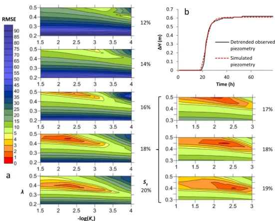
This approach was applied to infiltration events recorded in six piezometers (see the following), but only one simulation is detailed hereafter. The infiltration process considered here oc-curred on piezometer P42B after the rainfall event of October 22, 2009 (86.8 mm during 12 h with a maximum intensity of 21.8 mm h−1measured at Istres station) causing a rise of 0.62 m in the water table during the following 36 h (Fig.3). Assuming that the entire rainfall amount reaches the water table, a rapid application of the WTF method yields a first estimate of the specific yield of about 16%. As stated in sec-tion ‘Numerical analysis and implementation of the infiltra-tion model’, three parameters have to be inferred by uniform sampling of the parameter space and subsequent direct simu-lations: Ks, Sy, and λ. Regarding permeability (Ks), data mea-sured in some boreholes (Porchet1930; BRGM2016b) sur-rounding piezometer P42B (3 km) showed values between 5.10−4and 1.10−2m s−1. This preliminary work meant that

y = -0.0007x + 28.734 0 5 10 15 20 25 28.6 28.7 28.8 28.9 29.0 29.1 29.2 29.3 29.4 0 20 40 60 Rai nfal l (mm h -1) H ( m a sl) Time (h)

Fig. 3 The 22nd of October 2009 rainfall event observed at piezometer P42B. The dashed line represents the linear regression used to detrend and thus to remove the net groundwater drainage

contribution from the piezometric signal

the tested ranges of permeability (from 1.10−4to 5.10−2m s−1 every half order of magnitude) and porosity (from 12 to 20% every 2%) could be reduced, thus increasing the calculation speed. The pore-size distribution index (λ) was systematically tested between 0.2 and 0.5 (every 0.05) according to the mea-sured values of Rawls et al. (1982). To illustrate the approach, the misfit function (root-mean-square error based on hourly simulated and observed data) for piezometer P42B is present-ed in Fig.5a and shows a minimum error for a specific yield of 18% among the 210 simulations performed. But after a finer parameter space exploration—Kstested between 1.10−3and 9.10−2m s−1every 1/5th order of magnitude (1.10−3, 3.10−3, 5.10−3, 7.10−3, 9.10−3, 1.10−2,…); Sytested with 17, 18 and 19%; λ still tested between 0.2 and 0.5 every 0.05—the best simulation among these 150 new simulations (Fig.5b) was obtained for a permeability of 9.10−3m s−1, a pore-size distri-bution index of 0.5, and a specific yield of 17% (consistent with the 16% estimated at the beginning of this section by the WTF method).

Hydro-gravimetry results

Average value of Syat the aquifer scale

Figure6represents the results of the hydro-gravimetric survey (March 2015 data minus September 2014 data). The plot shows a correlation between gravimetric and piezometric var-iations (Δg versus ΔH). Shifts of the regression intercept reflect average WSC in the unsaturated zone of the Crau aqui-fer plus WSC of the reaqui-ference station (Pz10); hence, the three red dots, far from the linear trend (Pz20, Pz21 and 88F), pres-ent differpres-ent unsaturated zone storage variations from the rest of the aquifer and are not accounted for in the plotted linear regression. This is likely due to the clay beds, observed on stratigraphic logs (BRGM2016b), above the water-table var-iations of these zones. Using the 420 nm s−2m−1 gradient, derived from the Bouguer plate analytical expression (Eq.

10), it is possible to interpret the slope and the intercept of this linear regression in terms of specific yield and unsaturated zone water storage variation (mean and standard deviation) at the aquifer scale. Thus, not considering the three particular points, the Crau aquifer presents an average specific yield Sy of 12.3 ± 1.9%, and a variation of the unsaturated zone water storage ΔS between September 2014 and March 2015 of 0.121 ± 0.025 m. This average variation of unsaturated zone water storage was calculated considering 0.07 m of water-table fluctuation and no WSC in the unsaturated zone of the reference station (Pz10).

Point-scale measurements

The simplest way to correct the shift of the gravity measure-ments created by WSC in the unsaturated zone consists of

subtracting the intersection of the linear regression (Fig. 6). Doing this simplified average WSC correction, the application of Eq. (11) leads to eight unrealistic specific yield values out of the 24 estimates (Table2), because of the heterogeneous soil distribution over the Crau plain. Note also that the stan-dard deviations, computed using Eq. (12), are globally too high to characterize the precision of most of the values, espe-cially for piezometers presenting low water-table fluctuations between September 2014 and March 2015.

An alternative attempt was tried to perform a physically based correction ofΔS, using unsaturated zone storage data extracted from the Global Land Data Assimilation System (NASA 2016). The NOAH model (Rodell and Beaudoing

2013) provides monthly soil moisture values (up to 2 m depth) at a 0.25° × 0.25° grid resolution. The resolution and the prox-imity to the coastal shore only allow three meshes to be ex-tracted covering the north part of the Crau plain (Fig.1). Each piezometer within a NOAH mesh grid was directly corrected using the respective NOAH soil moisture variation ΔS (no improvements observed using any kind of interpolation of NOAH ΔS estimates), expect for Pz9 and Pz10 (in the absence of NOAH mesh at this precise location; Fig. 1), corrected using the neighboring mesh to the north. The mean NOAH soil moisture variation between September 2014 and March 2015 was about 0.2 m, in good agreement with the mean value discussed in the previous section (i.e. 0.121 ± 0.025 m). The southern and mostly unirrigated part of the Crau plain is not covered by the simulated NOAH soil mois-tures. However, considering the absence of substantial pedo-logic layers, the regional variation at this location should be lower than in the northern part of the Crau plain, in better agreement with the value obtained with hydro-gravimetric data. Using these NOAH unsaturated zone storage data to correct gravity measurements of piezometers within each grid cell (corrections represented by gray dots on Fig.6) provides new estimates of the specific yield (Table4) showing seven unrealistic values.

Discussion

Table4presents the specific yield values obtained by applying alternatively the three different methods. The following sec-tions discuss and compare these approaches.

Water-table fluctuation method

This simple method allows a straightforward estimation of the specific yield using all the piezometers of the Crau aquifer presenting daily piezometric data. The two main sources of uncertainties are (1) the vertical recharge estimate, which de-pends on the precipitation estimate and on the assumption that the entire precipitated amount reaches the water table without

substantial evapotranspiration, runoff, or unsaturated zone storage variations, and (2) the quantification of the net ground-water drainage rate. The hypothesis of an effective infiltration corresponding to the entire precipitation may produce overestimated specific yield values, especially because of pos-sible water retention in the unsaturated zone. Applying the WTF method on several major rainfall events mitigates the impact of this assumption, however. The results obtained by the WTF method (Table4) appear to be remarkably consistent with the ranges and locations of the few values reported in the literature (Table1; Fig.8).

The specific yield values of P29B and P42B, computed using only the few rainfall events that occurred during the studied period, are 8.3 ± 0.5% (n = 2) and 9.2 ± 1.5% (n = 3) respectively (Table4), which is very similar to the value com-puted using all the events measured at Istres meteorological station (Table3), i.e. 10.5 ± 3.5% (n = 8) and 10.2 ± 4.7% (n = 11) respectively. This confirms the reliability of the mean spe-cific yields computed using the few WTF interpretations per-formed on a period presenting major rainfall events. Table3

also shows that the heterogeneity of the rainfall distribution, and thus the choice of meteorological station impacts the re-sults, especially for the interpretation of smaller rainfall events. By using various interpretations however (see section ‘Method validation’), this uncertainty on rainfall value is much lower than that created by the variations in unsaturated

zone storage—standard deviation (SD), by considering the three meteorological stations (e.g. 0.8% for P42B) much low-er than the SD created by multiple WTF intlow-erpretations plow-er station (e.g. 4.6–6.6% for P42B; see Table3).

One-dimensional infiltration model

More time- and CPU-consuming than the WTF interpretation, this method, based on RE resolution, requires higher temporal resolution data and is, here, partly redundant with the WTF ap-proach (analysis of the same signal). Hence, the model application requires specific conditions that restrict the number of events which can be interpreted, as compared with the WTF method. Among the major infiltration events presented in Table2, only the hourly piezometric and weather records showing equivalent groundwater recession slopes before and after the piezometric rise were used. This constraint allows a clear detrending of the hy-draulic head time variation to obtain the pure infiltration signal.

In addition, similarly to the WTF method, some rainfall events can also present small precipitated volumes, which do not cause a piezometric rise, i.e. unsaturated zone water reten-tion (modified by evapotranspirareten-tion), producing some over-estimation of the specific yield. Consequently, in view of the limited number of events which can be interpreted, the uncer-tainty cannot be reduced by multiple applications of the meth-od as done for the WTF approach, except at P18B where two

y = 0.229x + 28.067 R² = 0.9634 27.5 28 28.5 29 29.5 30 30.5 31 31.5 0 1 2 3 4 5 6 7 8 H ( m a sl)

Groundwater net lateral drainage (D; mm d-1₎

y = 0.3873x + 16.263 R² = 0.9463 16 17 18 19 20 21 22 23 24 25 0 1 2 3 4 5 H (m asl )

Groundwater net lateral drainage (D; mm d-1₎

a

b

Fig. 4 Net groundwater drainage rate (D) as a function of the mean hydraulic head (H) of each WTF interpretation for piezometers a P42B and b P29B. Bold lines represent the topographic surface at each

piezometer, and error bars represent the amplitude of the water-table fluctuations of each studied infiltration event

Table 3 Results of multiple interpretations of large rainfall events by WTF method performed on P42B and P29B using the longest piezometric time-series with different meteorological stations. SD standard deviation

Borehole No. of events Mean Sy± SD per meteorological station Mean Sy± SD for

the three stations

Arles Istres Salon-de-Provence

P42B 11 9.0 ± 4.6% 10.2 ± 4.7% 10.7 ± 6.6% 9.9 ± 0.8%

Table 4 Results obtained using the three dif ferent ap proaches to infer specific yields. SD sta nd s for standard deviation Pie zo m ete rs Inf ilt rat ion mod el W T F m ethod Hydro-gravimetry BRGM code ID Network X (WGS8 4) Y (W GS84) Meteorological station Sy SD N o. of ev ents Sy SD Sy us ing m ean Δ SS y usi ng N OAH Δ S SD 09933X008 8 88F B R GM 4.93487 43.6801 1 Salon –– 27 .9 % 2. 4% 1. 1% 2. 6% 2. 3% 10192X009 4 94F B R GM 4.85507 43.4759 Istres –– 41 8. 1% 3. 3% –– – 09934X008 7 P18B B R GM 4.9633 43.65283 Sa lon 10.8% 0.8% 3 11.5% 0.9% 18.1% 20.6% 3.9% 09937X013 4 P19T B R GM 4.92382 43.60907 Istres –– 55 .0 % 1. 0% 17 .6 % −4.0% 34.4% 10192X009 5 P21B B R GM 4.81 14 43.5399 Istres –– 31 2. 4% 0. 5% −5.8% −13.2% 11.9% 09937X013 5 P23B B R GM 4.87195 43.57819 Istres –– 43 .5 % 0. 6% −15.5% −126.4% 178.7% 10193X015 1 P29B B R GM 4.89617 43.55071 Istres –– 28 .3 % 0. 5% 19 .0 % 8. 3% 17 .1 % 09937X013 3 P42B B R GM 4.86231 43.60812 Istres 17.0% – 29 .2 % 1. 5% −4.1% 4.1% 13.0% 09941X026 1 PZ1 SY MCRAU 5.05259 43.6546 Sa lon –– 36 .3 % 0. 6% 12 .1 % 15 .7 % 9. 4% 10197X055 4 PZ10 SYMCRAU 4.92877 43.45508 Istres –– 51 2. 3% 1. 5% –– – 10193X016 9 PZ1 1 SYMCRAU 4.90852 43.50369 Istres –– 21 2. 3% 1. 3% 51 .1 % 32 .4 % 29 .9 % 09936X014 1 PZ13 SYMCRAU 4.82014 43.5786 Istres –– 48 .5 % 0. 5% –– – 09936X013 8 PZ14 SYMCRAU 4.83842 43.63877 Istres –– 41 6. 5% 2. 2% –– – 09936X014 2 PZ15 SYMCRAU 4.78753 43.63581 Arles –– 51 0. 4% 3. 7% 26 .3 % 44 .9 % 29 .6 % 09945X026 4 PZ16 SYMCRAU 5.05782 43.6305 Sa lon –– 47 .5 % 2. 1% 6. 9% 12 .3 % 14 .2 % 09935X015 0 PZ17 SYMCRAU 4.73135 43.58632 Arles –– 34 .0 % 0. 4% –– – 09936X014 3 PZ18 SYMCRAU 4.77286 43.57821 Arles –– 28 .4 % 0. 6% 67 .7 % 8. 1% 96 .0 % 10193X017 0 PZ19 SYMCRAU 4.88875 43.52455 Istres –– 29 .1 % 1. 1% 6. 9% 3. 0% 6. 2% 09924X013 6 PZ20 SYMCRAU 4.66202 43.66105 Arles 6.5% – 33 .6 % 0. 6% −11 .9 % −7.4% 5.1% 09931X026 3 PZ21 SYMCRAU 4.72954 43.67315 Arles –– 22 .9 % 0. 8% 5. 7% 7. 3% 1. 8% 09934X009 1 PZ22 SYMCRAU 5.01796 43.67818 Sa lon –– 31 2. 7% 2. 8% −6.1% 14.6% 53.9% 09941X026 2 PZ23 SYMCRAU 5.08277 43.67305 Sa lon –– 52 6. 0% 6. 2% –– – 09935X015 1 PZ24 SYMCRAU 4.68413 43.59025 Arles 7.5% – 44 .7 % 1. 1% 37 .3 % 74 .3 % 42 .1 % 09937X015 6 PZ3 SY MCRAU 4.87098 43.63864 Istres –– 43 .5 % 0. 7% 1. 3% 10 .4 % 14 .5 % 09938X018 4 PZ5 SY MCRAU 4.99765 43.63866 Sa lon –– 21 1. 3% 0. 6% 15 .4 % 16 .8 % 3. 8% 09938X018 9 PZ6 SY MCRAU 4.9803 43.60608 Sa lon –– 2 10.2% 1.9% 10.0% 13.1% 4.8% 10194X025 7 PZ8 SY MCRAU 4.9666 43.53273 Istres –– 2 12.8% 0.7% −1.3% 5.7% 11 .1 % 10194X025 8 PZ9 SY MCRAU 4.96426 43.49161 Istres –– 6 5.6% 0.9% 31.0% 44.0% 20.8% 09938X018 7 Q UANT2 SYMCRAU 5.01988 43.64656 Sa lon –– 28 .0 % 0. 6% –– – 09937X015 9 Q UANT4 SYMCRAU 4.92471 43.64036 Istres –– 3 6. 9% 0. 4% 2. 5% 8. 1% 8. 8% 10194X025 9 Q UANT7 SYMCRAU 4.96884 43.55813 Istres 9.0% – 2 8.9% 0.2% 13.1% 19.4% 10.1%

events were simulated (with Ks= 10−3m s−1and λ = 0.45) leading to an average specific yield of 10.8 ± 0.8%, consistent with the WTF result (Table4).

Despite these limitations, the infiltration method can nev-ertheless be locally advocated for alluvial aquifers, especially in the absence of hydrodynamic parameters. Therefore, with

RMSE λ -log(Ks) 12% 14% 16% 18% Sy 20% 17% 18% 19% 0 0.1 0.2 0.3 0.4 0.5 0.6 0.7 0 20 40 60 ΔH (m ) Time (h) Detrended observed piezometry Simulated piezometry

a

b

Fig. 5 Parameter space 2D maps representing the RMSE function of the permeability Ks, the pore-size distribution indexλ, and the specific yield Sy of the 22nd of October 2009 rainfall event at a piezometer P42B; b observed and simulated piezometry Pz10 Pz11 P29B P23B P42B Pz15 P21B Pz18 Pz24 Pz3 Quant4 P19T Pz22 Pz1 Pz16 Pz5 P18B Pz9 Pz8 Quant7 Pz6 Pz19 Pz20 88F Pz21 y = 5.1348x + 5.4372 R² = 0.6788 y = 5.1454x - 2.5934 R² = 0.6849 -30 -25 -20 -15 -10 -5 0 5 10 15 20 -7 -6 -5 -4 -3 -2 -1 0 1 2 3 Δg (μGal) ΔH (m)

Fig. 6 Results of hydro-gravimetric surveys (September 2014 and March 2015) showing piezometric variations (ΔH) as a function of the gravimetric varia-tions (Δg) represented by black dots. Red dots represent the pie-zometers that are excluded from the regression, gray dots represent data after NOAH soil moisture correction, and dashed lines are the linear regressions performed on raw and corrected data

minimal data requirements, i.e. rainfall and water-table eleva-tion at a unique piezometer, this approach can provide a first complete set of key parameters, i.e. hydraulic conductivity and specific yield.

Hydro-gravimetry

As previously mentioned, rainfall events occurring before and during the hydro-gravimetric surveys reduced the piezometric level variations between the two campaigns (i.e. increased the errors of calculated specific yields), and increased water storage effects within the unsaturat-ed zone, which is difficult to ascertain. Hence, this tech-nical limitation impacts the point-scale results of this hydro-gravimetric approach (see section ‘Point-scale

measurements’). Nevertheless, using the mean and

NOAH soil moisture corrections (Fig. 6) improves the quality of the estimates provided by gravity variations due solely to water-table fluctuations, while preserving the same average regional specific yield (i.e., same re-gression slopes).

Comparison of the three methods

The infiltration model developed for this study to solve the RE involves costly time- and CPU-consuming simu-lations. In addition, the more difficult calibration process together with the specific conditions required (hourly pi-ezometric and weather records, equal groundwater reces-sion slopes before and after the piezometric rise) may limit the number of possible applications (see section ‘One-dimensional infiltration model: discussion’). In the specific case of the Crau plain, this method is less effi-cient as compared to the very straightforward application of the WTF method.

The interpretation of the hydro-gravimetric surveys yields a 12.3 ± 1.9% mean regional specific yield for the entire aquifer, consistent with the value of 9.8% obtained by averaging the values provided by the WTF approach (Table2), excluding the three points not accounted for in the hydro-gravimetric computation because of the local presence of clay beds (i.e. Pz20, Pz21, 88F; see section ‘Average value of Syat the aquifer scale’). The difference

may be due to the different prospecting areas for each method. Gravity measurements present lateral resolutions that increase tenfold with the water-table depth (McCulloh

1965), leading to averages 49 and 60 m radius of lateral resolution for the high and low water periods, respectively (1st and 2nd campaigns). To quantify the lateral resolution of the Syresulting from the two other methods (i.e. WTF approach and 1D infiltration model), it was proposed to apply the expression of the radius of action (R) of the water-table variation induced by uptake (Eq. 13, using

Dupuit’s formula; De Marsily1986) to estimate the radius of action of the rapid recharge event being studied: R t_{ð Þ ¼ 1:5} ffiffiffiffiffiffiffi T t S r ð13Þ Using an average T = 3.10−2m2_s−1_{(Seraphin 2016), the} average Sy= 0.98 obtained with the WTF approach, and the mean duration of the studied events t = 7.4 105_{s (i.e. 8.7 days;} Table2), leads to an average radius of action R = 231 m, as-suming that the uptake and infiltration processes involve the same physic. This suggests that the WTF approach and the 1D infiltration model would lead to specific yield estimates pre-senting lateral resolutions 3–4 times larger than the average one of the hydro-gravimetric method.

Figure7a,b presents comparisons of specific yield values obtained using mean or NOAH gravimetric corrections, and the WTF method. Although the use of the NOAH data does not yield a perfect agreement (11 points with a 5% difference out of the 17 realistic specific yield values inferred from gra-vimetry; Fig.7b), it provides a substantial improvement (as-suming that the most reliable Syestimates are obtained by the WTF method) as compared to the use of a mean soil moisture correction (9 points with a 5% difference out of the 16 realistic specific yield values inferred from gravimetry; Fig.7a). This suggests that relevant estimates of the soil moisture variations with a better resolution (model and measurements) should be able to improve the local interpretations of the gravity field campaigns. Although relevant regional specific yield and un-saturated zone water storage variations were ascertained, this method would be more accurate for larger aquifers. Given the lack of efficiency of the other two methods and the indepen-dent validation of the WTF approach (see section ‘Method validation’), this study considers the latter as the most reliable method to assess the spatial distribution of the specific yield for the Crau plain.

Specific yield spatial distribution and global

groundwater budget

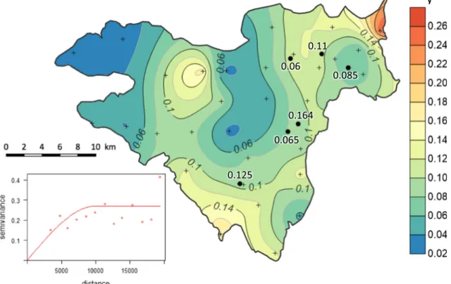
In the light of the comparison made in the previous section, the WTF results were used to describe the specific yield spatial distribution over the Crau aquifer. These 37 data were used in a geostatistical analysis with the BR^ statistical software (Ihaka and Gentleman1996). The interpolation of the logarithm of the specific yield data by kriging on a regular grid spacing (100 × 100 m) was performed by fitting a spherical model (sill = 0.05, range = 10,000 m, nugget = 0) to the empirical variogram (sample variance = 0.051; Fig.8), leading to a spatial distribu-tion of the specific yield (Fig.8) with a satisfying resolution and a 9.1% regional mean value (weighted by water content of each mesh). This new spatial distribution suggests an expected correlation between the specific yield and the geology. Most of

the values above 10% are located where the alluvial deposits are thick (above 20 m), and probably less cemented. Clay banks have been observed at the two piezometers (Pz20 and Pz21) in the north-west part of the Crau plain, explaining the low specific yield in this part of Fig.8.

The relevance of the specific yield spatial distribution ob-tained in this study can be verified using the global ground-water mass balance of the Crau aquifer which is written during a given time period:

∬∫hf

hiSyðx; yÞ dh dx dy ¼ ∫ tf

tiðRiþ Rnþ Qin−Qout−UÞdt ð14Þ

and involves all the groundwater fluxes circulating in the aqui-fer: the recharge by irrigation return flow (Ri), the natural

recharge (Rn), the upstream and downstream groundwater lat-eral flows (Qinand Qout), and the overall uptakes (U). The mass balance Eq. (14) is written, for an average year, over the period from 15 March (tiin Eq. 14) to 15 October (tf), corresponding to the irrigation period in order to maximize the specific yield effect (maximal water-table fluctuations). The right-hand side of Eq. (14) can be computed using the fluxes independently obtained using a stable isotope-mixing model (Seraphin et al.2016). According to this study, for the 7-month time period considered here, the recharge by irriga-tion return flow (Ri) and the natural recharge (Rn) were 4.92 ± 0.89 and 1.17 ± 0.50 m3_s−1_{, respectively. Note that, assuming} a constant infiltration process, Rnwas weighted using the av-erage proportion of precipitation during this time period

0.11 0.085 0.164 0.125 0.065 0.06

S

Fig. 8 Spatial distribution of the specific yield, obtained by interpolating (kriging) the results of the WTF method, and its associated variogram. Black dots represent the specific yield estimates of previous studies, and black crosses represent the location of the points used for the interpolation

0% 5% 10% 15% 20% 25% 30% 35% 40% 0% 5% 10% 15% 20% 25% 30% 35% 40% Sy by gr avim et ry Syby WTF 0% 5% 10% 15% 20% 25% 30% 35% 40% 0% 5% 10% 15% 20% 25% 30% 35% 40% Sy by g rav imetry Syby WTF

a

b

Fig. 7 Comparison of specific yields computed by the WTF method as a function of their counterpart from the hydro-gravimetry method using a aver-age soil moisture data and b NOAH soil moisture data. Dashed lines represent a 5% in-terval error (because of their ir-relevance, standard deviations of the gravimetric method are not represented)

(53.4% of the annual mean rainfall, computed with 1991– 2015 meteorological data). The uptakes (U) represent 1.52 ± 0.24 m3_s−1_{, the upstream groundwater lateral inflow (Q}

in), 0.48 m3 _s−1_{, and the natural discharge (Q}

out), 3.12 ± 0.20 m3s−1. Using these previous independent estimates, the right-hand side of the groundwater budget described in Eq. (14) yields a value of 3.57 ± 0.98 107_m3_{for the groundwater} storage variation in the aquifer between March 15th and October 15th. The left-hand side of Eq. (14) now can be com-puted using the specific yield spatial distribution obtained here to verify the consistency with the above calculation. Similar to the specific yield, the average water-table variations of 31 piezometers over this period (average variations computed between March 15th and October 15th for years 2013 and 2014, the period optimizing the number of piezometers with daily records) were interpolated by kriging. Then, the sum of the specific yield times the water-table variation for each mesh yields the required net overall groundwater storage variation in the aquifer between 15 March and 15 October (left-hand side of Eq.14). The value obtained by this calculation, 3.09 107 _m3_{, is in excellent agreement with the aforementioned} independent estimate (3.57 ± 0.98 107_m3_{) and reinforces the} relevance of this study.

Conclusions

Observed in monitored boreholes, multiple large infiltration processes caused by large precipitation events were interpreted in terms of specific yield by means of the WTF method and a 1D vertical numerical model solving the RE in the unsaturated zone. Both of these methods are sensitive to the assumption of recharge by the entire rainfall volumes and the heterogeneity of the precipitation events, but the WTF interpretation of multiple major events for each piezometer yields relevant results and reduces the impact of these limita-tions. Assuming that the most reliable Syestimates are obtain-ed by the WTF method, and despite the low signal, the gravi-metric method provides a valuable regional specific yield con-sistent with the results of the WTF method. The local bias of the hydro-gravimetric method, due to soil water storage, can be partially eliminated using widely available NOAH soil moisture data, but does not lead to relevant local specific yields in this case. Since this method is redundant for Sywith the WTF approach, the infiltration method, which is more time-consuming, should be limited to areas where additional hydraulic conductivity values are desirable (unsampled areas). The range of local specific yields obtained by the WTF meth-od (2.9–26%) is in line with the scarce data available so far. Hence, the first regionalized map of the specific yield of this aquifer of major economic importance is proposed here, mak-ing it possible to build an accurate transient model based on parameter values independent from any prior hydrogeological

modeling. Tested by means of a simple mass balance calcula-tion over the Crau plain, the estimates obtained here are con-sistent with the overall groundwater budget recently calculat-ed using stable isotopes, showing the robustness of these methods. Additional parameters can be obtained by the alter-native approaches proposed here: the infiltration model pro-vides permeability, the WTF method offers the opportunity to independently estimate mean recharges (using the relationship between net groundwater drainage and hydraulic head; see section ‘Method validation’), and hydro-gravimetry can esti-mate an average soil moisture variation. In a context of cliesti-mate change implying more frequent extreme rainfall events, the authors believe that these approaches would produce more accurate and relevant results for other large unconfined aqui-fers, compared to the commonly performed spatial calibration of the specific yield through hydrogeological modeling. Acknowledgements This study is part of a PhD funded by the SYMCRAU and the PACA region. It has been supported by CNRS-INSU, through the SICMED-CRAU research project. We thank the CNRS-INSU national facility RESIF-GMOB for providing the Scintrex CG5 gravimeters. We thank M. Peeters and the three other reviewers for their constructive comments which helped in improving the manuscript.

References

Albinet M, Bonnet M, Colomb E, Cornet G (1969) Carte hydrogéologique de la France, 993-1019, Istres-Eyguières, Plaine de la Crau [Hydrogeological map of France, 993-1019, Istres-Eyguières, Crau plain]. 1/50000. BRGM, Orleans, France ANTEA (1995) Municipality of Salon de Provence (13) - Application for

authorization to use water taken from the natural environment [Commune de Salon de Provence (13) - Demande d’autorisation d’utilisation d’eau prélevée dans le milieu naturel].

Bader J-C, Saos J-L, Charron F (2010) Modèle de ruissellement, avancement et infiltration pour l’irrigation à la planche Sur un sol recouvrant un sous-sol très perméable [Runoff, advancement and infiltration model for board irrigation method on a soil covering a highly permeable subsoil]. Hydrol Sci J 55:177–191.https://doi.org/ 10.1080/02626660903546050

Becker M, Meyssignac B, Xavier L, Cazenave A, Alkama R, Decharme B (2011) Past terrestrial water storage (1980–2008) in the Amazon Basin reconstructed from GRACE and in situ river gauging data. Hydrol Earth Syst Sci 15:533–546. https://doi.org/10.5194/hess-15-533-2011

Beilin J (2006) Apport de la gravimétrie absolue à la réalisation de la composante gravimétrique du Réseau Géodésique Français [Contribution of absolute gravimetry to the realization of the gravi-metric component of the French Geodetic Network]. Inst. Géographique National, Saint-Mandé, France

Berard P, Daum JR, Martin JC (1995) BMARTCRAU^: actualisation du modèle de la nappe de la Crau [BMARTCRAU^: updating the Crau aquifer model]. BRGM, Orleans, France

Beven K (1993) Prophecy, reality and uncertainty in distributed hydro-logical modelling. Adv Water Resour 16:41–51

Boissard G (2009) Geological and hydrogeological synthesis. Quantitative assessment of the impact on the water resource [Synthèse géologique et hydrogéologique. Évaluation quantitative de l’impact sur la ressource en eau], Report F, ICF Environnement.