Social, economic and policy analysis of recreational fisheries in Flanders

Limburgs Universitair Centrum Center for Statistics

Social, economic and policy analysis

of recreational fisheries in Flanders.

By:

Mario Cools

Thesis submitted in partial fulfilment of the requirements for the degree of

Master of Science in Applied Statistics

Academic year 2004-2005

Supervisor: Dr. Alain De Vocht Internal supervisor: Dr. Ariel Alonso Abad

Abstract i

Abstract

Social sciences revealed that there exists a great diversity among anglers in terms of social and economic profile. Different angling groupings can be made based on resource use, experience, investment or centrality of fishing to the total lifestyle. Thus, the main objective of this report is to study the diversity in the social economic profiles of the Flemish anglers and to find the main differences between different types of anglers. The models used to find these differences were cluster analysis, discriminant analysis, decision trees (binary and k-child trees) and zero-inflated poisson regression. There was a clear separation between eel and predator anglers on the one side, and the other types of anglers on the other site. The catch-and release anglers were thus clearly different from anglers who fish to consume. The overall willingness to pay was generally higher when anglers spend more money on their fishing equipment and on magazines. Finally, a general framework for recreational fisheries policy was set up.

Acknowledgement ii

Acknowledgement

This report has been accomplished with considerable support from several people. I would like to take the opportunity to gratefully acknowledge their support.

First, I would like to thank Alain De Vocht for his guidance and support during the writing of this report. The discussions around the subject of recreational fisheries were extremely helpful in pointing out the direction of this report.

I would also like to express my gratitude to Ariel Alonso Abad and Geert Molenberghs for their statistical methodological support.

Finally, I would like to acknowledge my parents, friends and girlfriend for their continuous patience and understanding.

Table of content iii

Table of content

3.1 Exploratory data analysis 4

3.2 Cluster analysis 4

3.3 Canonical discriminant analysis 6

3.4 Decision trees 6

3.5 Zero-inflated poisson regression 9

4. Results and interpretation 11

4.1 Exploratory data analysis 11

4.2 Cluster analysis 13

4.3 Discriminant analysis 14

4.4 Decision trees 15

4.5 Zero inflated poisson regression 21

5. Discussion 24

6. A framework for fisheries policy 25

7. Conclusion 28

References 29

Appendix 32

A. SAS Code for the zero-inflated poisson regression 32

B. Results EDA for the different angling types 33

C. Results EDA for the willingness to pay (willing or not) 36

D. Discriminant analysis 37

Introduction 1

1. Introduction

The last years the interest in the human dimensions of fisheries management increased. Policy makers need to know what anglers think and do regarding fishery resources. Therefore various methods must be used in order to collect data to describe, understand and predict angler behaviour1.

In the past, fishing was a source of revenue for many people2. Nowadays, in the developed world (e.g. North America, Belgium, United Kingdom), full-time commercial food fisheries have largely disappeared and recreational, leisure or ‘sport’-fisheries became the dominant components of evolved inland fisheries systems. Consequently, fisheries management in industrialized countries focuses almost exclusively on recreation and conservation3.

Recreational fisheries have economic, social, cultural and ecological benefits, as for instance discussed by Arlinghaus, R., Mehner, T. and Cowx, G (3). The net economic value to anglers can be determined through the Contingent Valuation Method (CVM)4. This net economic value, or consumer surplus, is defined as the difference between what a commodity, like recreational fisheries, actually costs, and what anglers would be willing to pay for it5. The CVM involves asking a sample of the relevant population their willingness to pay (WTP) for an improvement or their willingness to accept compensation (WTA) for a deterioration6,7. In this report WTP will be an indication for how much anglers are willing to pay above the current price of a public fishing license.

The number of recreational anglers in Flanders is estimated as 175 000 which corresponds to 2.9% of the Flemish population8,9. About 35%, or 61 245 anglers, fishes on public waters. This number decreased the last decennium. It is worth mentioning that this decreasing trend has an impact on the normal and the youth fishing license, but not on the special fishing license. One of the reasons is that the more expensive special fishing license allows wading fishing and boat fishing. Figure 1 shows this trend in the number of public fishing licenses10.

In Belgium, the Law on the river-fishery (July 1, 1954) lays the foundation for the organisation of the public fishery. Public waters are described as navigable and floatable watercourses, of which the conservation is chargeable to the state or his rightful claimant.

Introduction 2 For fishing on public water, a public fishing licence of the Flemish community is required,

which can be bought in the post offices. In 2003, the price of a normal fishing license was 11.60 euro.

Figure 1: Number of public fishing licences (Source: Dumortier et al. 2005)

Social sciences revealed that there exists a great diversity among anglers in terms of social and economic profile3. Thus, different angling groupings can be made based onresource use (type of equipment, species sought, harvest rate), experience (years of experience, frequency of fishing), investment (equipment owned, fishing expenditures) or centrality of fishing to the total lifestyle (club memberships, magazine subscriptions, maximum fishing trip distance, etc…)6.

The main objective of this report is to study the diversity in the social economic profiles of the Flemish anglers and to find the main differences between different types of anglers, but also the difference between anglers in overall willingness to pay will be modelled. Finally, this report will outline a general framework for recreational fisheries policy.

The data 3

2. The data

The data was collected by a last year student Applied Economical Sciences at the LUC11 who did a survey to investigate social and economical information about the recreational fisheries on public water in Flanders.

The studied population was the 61 245 Flemish anglers who bought a public fishing licence of the Flemish community in 2003. The anglers who fish on Flemish public waters without having a license (illegal fishermen) were not in the sample frame.

From the 61 245 target units a systematic sample of 10 000 people was taken. This was done by sampling every 6th person from the list of addresses of the owners of a public fishing licence of the Flemish community. This list was ordered by the date the anglers bought their fishing licence. Individuals not living in the Flemish community (for instance Dutch, French, or Walloon people) and several individuals under 14 were removed from this list. So finally, 10000 persons were selected and send a questionnaire11.

The real sample, after deleting the wrong addressed and those who just send it back with some remarks, contained 9492 individuals. Table 1 shows some features of this survey. The final dataset consisted of 3001 observations, containing information about the socio-economic status, experience, WTP and WTA of the Flemish anglers.

Table 1. Sample size, sampling interval and response rate

Population Sample True sample Sampling interval Number of responses True interval Response rate (%) (1) (2) (3) (4)=(1)/(2) (5) (6)=(1)/(5) (7)=(5)/(3) 61245 10000 9492 6.12 3001 20.41 31.62%

For the analysis of this report all anglers (ten anglers) which had another angling discipline than the known angling disciplines in Flanders, were removed from the dataset. The self-employed anglers were recoded as executives because being self-self-employed was not an answer option in the survey.

Statistical methodology 4

3. Statistical methodology

The statistical packages used in the analysis of this report were SAS 9.1 and R 2.1. A lot of statistical techniques were already used in the reports of Vandecruys11 and Govarts12. Vandecruys is a good reference work for basic statistics around the dataset used in this report. The focus in the report of Govarts lies on the modelling of the ordinal dependent variable “overall willingness to pay”.

3.1 Exploratory data analysis

In order to get a general picture of the data, different exploratory data analysis techniques were used. These techniques helped in finding e.g. the shape of distribution or finding outliers. Since the main focus on this report lies on finding differences between different types of anglers, basic descriptive statistics (means, median, trimmed mean) were calculated for each angling type for the continuous variables. For the categorical variables, frequency tables were constructed. As arithmetic means are particularly sensitive to extreme WTP values, median WTP or 5% trimmed means are recommended as measures of central13.

3.2 Cluster analysis

Cluster analysis is a multivariate statistical method to group data points into clusters or groups suggested by the data14, thus not defined a priori, so that the resulting clusters of objects exhibit high internal (within-cluster) homogeneity and high external (between cluster) heterogeneity. Thus, if the classification is successful, the objects within clusters will be close together when plotted geometrically, and different clusters will be far apart15.

Disjoint cluster analysis assigns each observation in only one cluster. First the observations are arbitrarily divided into clusters, and then observations are reassigned one by one to different clusters on the basis of their similarity to the other observations in the cluster. The process continues until no items must be reassigned14. This inter-object similarity can be measured in different ways. The three dominating methods in cluster analysis are: correlational measures, distance measures and association measures15.

Statistical methodology 5 The similarity measure that is used in here is the Euclidian distance between two p-dimensional observations16. Letx′ ⎡= ⎣x x₁, ₂,...,x_p⎤_⎦,y′ ⎡= ⎣y y₁, ₂,...,y_p⎤_⎦, then the Euclidian distance between point x and y is given by

( )

(

) (

)

(

)

(

) (

)

1 1 2 2

, ... _{p p}

d x y = x −y + x −y + + x −y = x y− ′ x y− (3.1) The advantage of using the Euclidian distance in stead of the statistical distance, is the fact that for the Euclidian distance no prior knowledge of the distinct groups is needed16.

In its simplest version, the K-means process is composed of these three steps17: 1. partition the items into K initial clusters

2. proceed through the list of items, assigning an item to the cluster whose centroid is nearest, recalculate the centroid for the cluster receiving the new item and for the cluster losing the item.

3. Repeat step 2 until no more reassignments take place.

Rather than starting with a partition of all items into K preliminary groups in step 1, we could specify K initial centroids (seed points) and then proceed to step 2.

There exists no standard objective selection procedure to determine how many clusters exist15. Combining the pseudo F statistic with the cubic clustering criterion (CCC) can provide a fairly reliable determination for the cluster number18. Do note that the CCC is not trustworthy when covariates are highly correlated19.

The cluster analysis is computed by the SAS-procedure FASTCLUS. This procedure uses a sequential threshold method. The procedure begins by selecting cluster seeds which are used as initial guesses of the means of the clusters. The first seed is the first observation in the data set with no missing values. The second seed is the next complete observation that is separated from the first seed by a specified minimum distance. After all seeds have been selected, the program assigns each observation to the cluster with the nearest seed15. This FASTCLUS procedure performs well on datasets containing 100 or more observations14,19. In order to perform the cluster analysis all ordinal and continuous variables were standardized, so that they had equal weights, and all nominal variables were recoded in dummies.

Statistical methodology 6

3.3 Canonical discriminant analysis

Canonical discriminant analysis is a dimension-reduction technique with as primary purpose to separate populations16. It is able to find linear combinations of the quantitative variables that provide maximal separation between the classes or groups, but it can also be used to classify19.

It is not necessary to assume that the g populations are multivariate normal, but it is assumed that thep× population covariance matrices are equal and of full rankp 19:

1 2 ... g

∑ = ∑ = = ∑ = ∑ (within structure20

) (3.2)

The socio-economic variables were selected to discriminate between different types of anglers. If the spearman correlation between discriminating variables was higher than 0.5, then the variable with the least missing observations was selected. All categorical variables were recoded as dummies. In order to evaluate the discrimination power, one could look at the misclassification error.

It is noteworthy that there is very little theory available to handle the case in which some variables are continuous and some variables are categorical. Therefore it is necessary to interpret the results with caution16.

3.4 Decision trees

3.4.1 Definitions

Decision tree induction is a well established technique, which finds his origin in artificial intelligence21. A decision-tree-based model is set of classification rules that partition a data set into mutually exhaustive and non-overlapping subsets22. A tree is developed by recursively splitting the sample on predictor variables with the aim to produce groups that are as homogeneous as possible in terms of the response variable21. Advantages for choosing a tree-based approach above traditional models are: tree-tree-based models can handle interactions among variables in a straightforward way, they can easily handle a large number of predictor variables, and they do not require assumptions about the distribution of the data14 (thus it is a nonparametric approach).

Statistical methodology 7

The root of a tree is the entire data set, the subsets and subsubsets form the branches of the tree. Subsets that meet a stopping criterion, and thus are not partitioned, are leaves. Any subset in the tree, including the root or leaves, is a node. A node where a split is formed is called a parent node, the subsequent nodes are called child nodes. Terminal nodes are nodes that are not split further (thus a terminal node is the same as a leaf)23.

The following conditions will terminate the algorithm of recursively splitting nodes: the maximum tree depth that has been reached, the fact that there is no significant predictor variable left to split the node, the fact that the number of cases in the terminal node is less than the minimum required number of cases for parent nodes, and finally the fact that if the node was split, the number of cases in one or more child nodes would be less than the minimum required number of cases for child nodes24.

There exist mainly two types of tree-based models: there are classification tree models, and regression tree models. The basic difference is the scale of measurement of the response variable. In a classification tree model the response variable is assumed to be categorical and measures of homogeneity appropriate to categorical data are used to determine the splits in the tree. In a regression tree the response variable is assumed to be continuous and measures of homogeneity relevant to the distribution of a continuous variable are used to determine the splits in the tree22.

3.4.2 Binary recursively partitioning

The RPART-procedure constructs a binary decision tree by recursively partitioning the data, in forward/backward stepwise manner. The idea is to first grow a saturated tree. A tree is saturated in the sense that the nodes subject to further division cannot be split25. The terminal nodes are then recombined or “pruned” upwards to an optimal size tree. The degree of pruning is determined by cross-validation using a cost-complexity function that balances the apparent error rate with the tree-size26.

The partitioning process is based on splitting rules. The best possible variable to split the rood node is the one that results in the most homogeneous and most pure child nodes. The

Statistical methodology 8 goodness of a split can be measured by the reduction in impurity. The best split is then obviously the split with the largest reduction in impurity24.

When no stopping conditions are defined the partitioning process will continue until a saturated tree is obtained and ‘pure’ classification will be achieved. However the saturated tree is usually too large to interpret26. Therefore it is typically to define stopping conditions. Here, a minimum of 10 individuals for a parent node, and at least 5 individuals for a terminal node, were specified.

The optimal tree is the tree that corresponds to the complexity parameter that gives a minimum cost for the new data23. Often there are several trees with costs close to the minimum, then the smallest-sized tree whose cost does not exceed the minimum cost plus 1 times the standard error of the cost will be chosen25. This is the ‘1 SE-rule’.

When no separate test sample is available, V-fold cross-validation is a useful alternative. A specified V value, here 10, determines the number of random subsamples, as equal in size as possible, that is formed from the earning sample. The binary tree is then computed V times, each time leaving out one of the subsamples from the calculations. The subsample that was not used in the calculations serves then as a test sample for cross-validation. The CV costs computed for each of the V test samples are then averaged to give the V-fold estimate of the CV cost25.

One of the benefits of using a classification or regression tree is that these methods can easily handle missing values. The approach used in this report was the approach of surrogate slits: information in other predictors is used as auxiliary information in order to decide whether an observation has to be sent to the left or to the right daughter node. The predictor that is most similar to the original predictor in classifying the observations will be used in the first surrogate split. It is possible that the predictor that yields the best surrogate split has also missing values. Then for the remaining observations that are not split yet, there will be looked for the second best, and so on. A maximum of 5 surrogate splits will be used. If all surrogates are missing, then the observation is sent in the majority direction.

Statistical methodology 9

3.4.3 Chi squared automatic interaction detection tree (CHAID)

Chi squared automatic interaction detection (CHAID) in an non-binary k-child tree-method for classifying categorical data28. The decision tree is constructed by partitioning the data set into two or more child-nodes repeatedly. After the dataset is partitioned according to the chosen predictor variable, each subset is considered for further partitioning using the same criterion that was applied to the entire dataset. Each subset is portioned without regard to any other subset. This process is repeated until some stopping criterion is met.14 The predictor variable used to form a partition, is chosen to be the variable that is most significantly associated with the dependent variable according to a chi-squared test of independence in a contingency table30.

The algorithm used to perform the CHAID classification tree was the SAS macro treedisc. This algorithm is similar to the CHAID algorithm described in Kass29, but some unclearness is clarified30.

Because CHAID-trees become rapidly difficult to interpret, the following stopping conditions were defined to be able to make meaningful interpretations and graphical representations. Here, a minimum of 100 individuals for a parent node, and at least 50 individuals for a terminal node were specified. The maximum tree-depth of 3 was defined.

Three types of predictors can be defined in the tree procedure: nominal predictors, ordinal predictors or ordinal predictors with a floating category. The latter can be used to handle missing data, because if an ordinal floating predictor has missing values, then the floating category will be the missing value. Thus a separate category is used for missing data30.

3.5 Zero-inflated poisson regression

Zero-inflated Poisson (ZIP) regression is a model for count data with excess zeros. It assumes that with probability p the only possible observation is 0, and with probability1− , a p

( )

Poisson λ random variable is observed. Both the probability p and the mean number λ may depend on covariates31.

Statistical methodology 10 Thus 0 i Y = with probability

(

)

(

)

Moreover, for covariates matrices B andGthe parametersλ=

(

)

(

)

satisfy32:

( )

log λ =Bβ (3.5)

( )

(

(

)

)

logit p =log p 1−p =Gγ (3.6)

In order to model the overall willingness to pay as a zero inflated response variable, the value-scale of 1-9 has to be recoded in a value-value-scale of 0-8.

The model building process is the following: first each model is selected with one and the same predictor variable for the zero-inflated as for the count part. If the variable is significant for one of the parts, it is added to a list, with notion for which part(s) it is significant. After all predictors are tested, the full model, with the remaining predictors that are in the list, is modelled. The non-significant variables are then removed in a backward way. Note that making an inference for a nominal variable is a nontrivial task because of the use of dummies. Those nominal scaled variables, where at least forty percent of the dummies is significant, are left in the model. Then finally some economic meaningful two way interactions are tested.

In order for model comparison, the Akaike Information Criterion (AIC) can be used33. The SAS-code used to model the zero-inflated poisson regression is appended.

Results and interpretation 11

4. Results and interpretation

4.1 Exploratory data analysis

4.1.1 General comments

As indicated earlier, the main focus on this report lies on finding differences between different types of anglers. The following table shows the frequencies of the different angling types. More than half of the anglers in the dataset are coarse anglers.

Table 2: Frequency table of the different angling types

Angling type Frequency Percent Coarse fishing 1560 52.49 Carp fishing 524 17.63 Fly fishing 22 0.74 Boat fishing 24 0.81 Match fishing 188 6.33 Eel fishing 248 8.34 Predator fishing 406 13.66

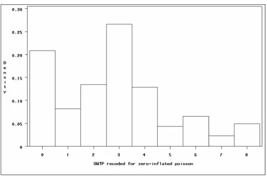
Since also the willingness to pay will be modelled, it is meaningful to show the excess of zero counts, by making an histogram of the recoded overall willingness.

Results and interpretation 12

4.1.2 EDA on angling types

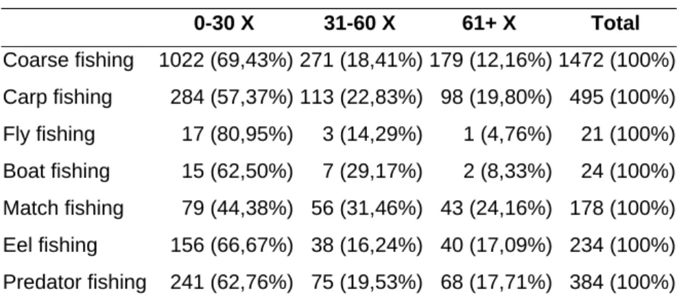
Table 3 shows the frequency table of angling type × frequency of fishing. The other frequency tables are presented in the appendix B1. Table 3 shows that carp anglers and match anglers are exercising their hobby more often than the rest. Coarse and fly anglers fish the leastfrequently.

Table 3: Frequency table angling type × frequency of fishing

0-30 X 31-60 X 61+ X Total Coarse fishing 1022 (69,43%) 271 (18,41%) 179 (12,16%) 1472 (100%) Carp fishing 284 (57,37%) 113 (22,83%) 98 (19,80%) 495 (100%) Fly fishing 17 (80,95%) 3 (14,29%) 1 (4,76%) 21 (100%) Boat fishing 15 (62,50%) 7 (29,17%) 2 (8,33%) 24 (100%) Match fishing 79 (44,38%) 56 (31,46%) 43 (24,16%) 178 (100%) Eel fishing 156 (66,67%) 38 (16,24%) 40 (17,09%) 234 (100%) Predator fishing 241 (62,76%) 75 (19,53%) 68 (17,71%) 384 (100%)

The following table shows the basic measures of central tendency for the distance to the fishing location. Boat fishers and fly fishers cover the largest distance to their fishing spot. Coarse fishers and eel fishers travel the least. The tables for the other continuous variables are presented in appendix B2.

Table 4: Basic measures of central tendency for the variable “distance to the fishing location”

Mean Standard error 5% Trimmed mean Standard error Median Coarse fishing 16.21 0.46 13.97 0.38 10.00 Carp fishing 19.83 0.94 17.07 0.79 15.00 Fly fishing 38.10 7.32 36.67 8.12 30.00 Boat fishing 34.05 5.15 32.28 4.97 32.50 Match fishing 24.16 1.49 22.10 1.42 20.00 Eel fishing 16.79 1.34 13.47 0.96 10.00 Predator fishing 21.85 1.17 19.01 1.07 15.00 Total 18.39 0.37 15.79 0.30 12.00

Results and interpretation 13

4.1.3 EDA on the overall willingness to pay

The main conclusions of the frequency tables (Appendix C1) and summary statistics (Appendix C2) for the overall willingness to pay, expressed by a dummy variable, indicating whether anglers are willing to pay more than the current price for a public fishing license (1) or not (0), are the following: retired and unemployed anglers are least willing to pay; the higher the salary, the more the anglers are willing to pay. The more experienced the angler is, and consequently the older the angler is, the smaller the willingness to pay. The more satisfied the angler, the more he is willing to pay.

4.2 Cluster analysis

When the only the socio-economic profile of the angler was used to perform the cluster analysis, the number of clusters suggested by the data would be 1 (based on the CCC and Pseudo f statistic). Thus, it would be best not separate the data into clusters. When the WTP and WTA data were also added to the cluster analysis, the CCC and Pseudo F statistic suggested two or three clusters.

The following frequency table shows the relationship between the clusters and the different angling types. There seems to be no clustering of certain angling types into a specific cluster.

Table 5: Frequency table of the obtained clusters from the disjoint cluster analysis × angling type

Coarse Carp Fly Boat Match Eel Predator Total

Cluster 1 795 (59.95%) 203 (14.54%) 11 (0.79%) 10 (0.72%) 61 (4.37%) 137 (9.81%) 179 (12.82%) 1396 (100%) Cluster 2 488 (51.21%) 165 (17.31%) 3 (0.31%) 6 (0.63%) 83 (8.71%) 69 (7.24%) 139 (14.59%) 953 (100%) Cluster 3 277 (44.46%) 156 (25.04%) 8 (1.28%) 8 (1.28%) 44 (7.06%) 42 (6.74%) 88 (14.13%) 623 (100%)

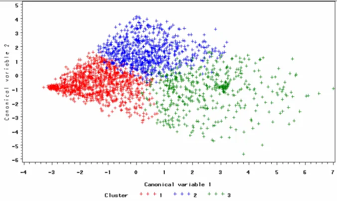
When a canonical discriminant analysis is performed on the obtained clusters, by using the same predictor variables as used for the disjoint cluster analysis itself, then two canonical variables are obtained that optimally discriminate the clusters.

The following picture (Figure 3) is the scatter plot of the two canonical variables for each of the clusters. It is clear that the clusters are almost perfectly disjoint. This is expected, because the purpose of disjoint cluster analysis is finding non-overlapping clusters.

Results and interpretation 14

Figure 3: Scatterplot of the two canonical variables for each of the three clusters

4.3 Discriminant analysis

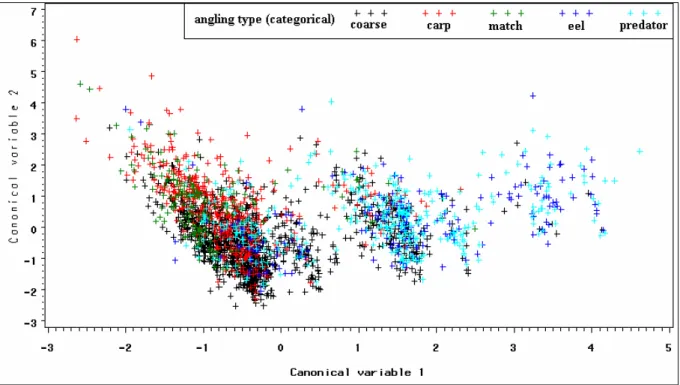
The discriminant analysis was performed on a reduced dataset: the fly and boat fishers were removed from the analysis, because there were to few anglers of this type. When discriminating between the remaining 5 types of anglers, it is important to note that from the 2926 observation that angling type defined, 540 observations (18,46%) had missing values and thus were removed for the analysis.

Since there were 5 classes to discriminate between, 4 canonical variables were obtained. The scatterplots between these four canonical variables show that the discrimination between the different types of anglers is very poor. Though, it can be seen that most of the eel and predator anglers are discriminated from the rest (figure 3). When the linear combinations are used for classification the overall misclassification error was 39.82% if the priors were based on the data itself. The detailed classification table can be found in appendix D.

Results and interpretation 15

Figure 3: Scatterplot of the two first canonical variables for each of the five angling types

4.4 Decision trees

4.4.1 Binary decision trees Angling type

When all the available variables were used for performing a classification tree analysis for the angling type, the obtained saturated tree had 9 terminal nodes. Since both the cost and the complexity of the tree had to be taken into account, a plot was made of the cost versus the size of the tree (figure A1 Appendix E1). From this plot there can be seen that the tree with the smallest cost is the saturated tree. However, when complexity is taken into account, the 1 SE-rule is fulfilled for the tree with 6 terminal nodes. The cost of this tree is approximately 0.91. When pruning the saturated tree to a complexity parameter (cp) of 0.015 (which corresponds to a tree size of 6), the final classification tree was obtained, as shown in figure 4. The surrogate splits used, in case of missing values in this tree, are given in table A25 (Appendix E1).

Results and interpretation 16

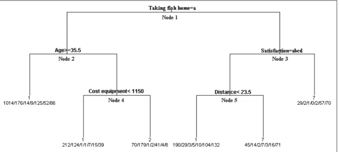
Figure 4: Classification tree for angling type, obtained by rpart

In the classification tree analysis 2972 observations were used in stead of 2991, because for 19 individuals the angling type (the response variable) was missing. From figure 4 we can see that the first decision rule is based on the fact whether the angler takes the caught fish home or not. When the angler does not take the fish home, age and cost equipment allows us to partition this type of anglers further. When the anglers do take fish home, satisfaction, and in a minor degree the distance to the fishing spot, are of importance to determine the angling type.

The first decision rule, node 1, splits anglers that do not take fish home (2180 anglers) from the ones that do take fish home (792 anglers). 40 individuals had missing values with respect to this variable, and because no surrogate splits were available, the missing values were sent in the majority direction.

The first group was divided again, node 2, in those that were at least 35.5 years old (1476 anglers) and those that were younger than 35.5 years (704 anglers). One surrogate split was performed (table A25 appendix E1). The first group was then not divided anymore, and thus this was a terminal node. The anglers in this group were primarily coarse fishers. The second group was further divided into the anglers that paid less than 1150 euro for their fishing gear (399 anglers), this group represented primarily coarse fishers, and the anglers that paid at least 115 euro for their fishing great (305 anglers). Carp anglers were primarily represented in this group.

Results and interpretation 17

The group of anglers that take their caught fish home is divided into the group that are not completely unsatisfied (631 anglers) and the group that is completely unsatisfied (161 anglers). The latter represent primarily predator anglers. The first group is divided again according to the distance the anglers cover to go to their fishing spot. If the distance is smaller than 23.5 km, the anglers (473) are primarily coarse fishers. If the distance is longer, the anglers (158) are primarily predator fishers.

The main predictor for the angling type is the fact whether the anglers take the caught fish home or not. This corresponds with the fact whether the angler deploys the catch and release philosophy or not. It is noted that 4 categories did not dominate an endnote. The boat and fly fishers represent only about 20 anglers each, so there can be expected that they were not dominating an endnote. The match fishers were primarily in the big group of coarse anglers that did not take fish home and were older than 35.5. Eel fishers were clearly located in the part of the anglers that take their fish home. They seem to group together with the predator fishers.

Angling satisfaction

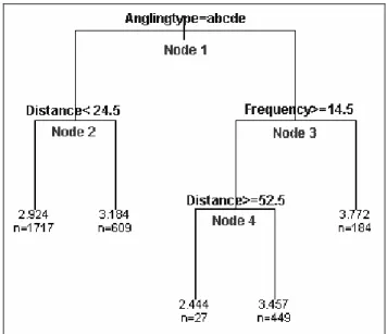
When performing a binary regression tree analysis for the satisfaction of the anglers, the saturated tree was already very easy to interpret, so pruning was not necessary. The surrogate splits, in case of missing values, are given in table A26 (Appendix E1).

Results and interpretation 18 Figure 5 shows the binary regression tree for the angling satisfaction. Angling type is the most important predictor for the satisfaction. It splits the eel and the predator fishers (who fish mainly for consumption) from the other types of anglers. The latter are a little bit more satisfied (1 is best, 5 is worst) when the distance, they have to travel to the fishing spot, is smaller than 24.5 km. If eel and predator anglers go 14.5 times or more on a fishing trip, they are more satisfied then the ones that go fewer times. When the eel and predator anglers travel 52.5 km or more to their fishing spot, they are remarkable more satisfied than the ones that travel less.

Overall willingness to pay

When performing a binary regression tree analysis for the overall willingness to pay, the saturated tree was already very easy to interpret, so pruning was not necessary. The surrogate splits, in case of missing values, are given in table A27 (Appendix E1).

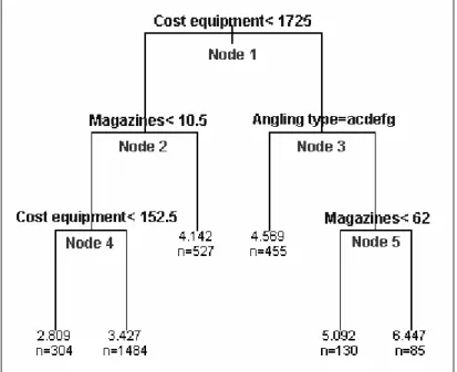
Figure 6: Regression tree for the overall willingness to pay, obtained by rpart

The most important variable in describing the willingness to pay is the cost of the fishing equipment. Those that have paid less than 1725 euro for their equipment are clearly less willing to pay than the anglers that have paid 1725 or more. For the anglers that paid less than 1725 euro it is important to see how much they spent on magazines. If they spent 10.5 euro or more, they were willing to pay on average ± 11.4 euro more for their fishing license.

Results and interpretation 19 The ones that spend less than 10.5 euro on magazines can be subdivided again in the ones that have an equipment that costs less then 152.5 euro, and those whose equipment is worth at least 152.5 euro. The first are willing to pay on average ± 4.5 euro more. The latter are willing to pay on average ± 7.1 euro more for their fishing license.

The group of anglers that spent at least 1725 euro on their fishing gear can be subdivided depending on the angling type. If these anglers were not carp fishers, then their average willingness to pay was ± 15.7 euro. The carp anglers that paid at least 1725 euro can be subdivided according to their expenses on magazines. If they spent less than 62 euro on magazines they were on average willing to pay ± 20.9 euro more for their fishing license. If they spent at least 62 euro on magazines, they were willing to pay on average 34.5 euro more.

Overall willingness to pay – dummy

A dummy variable was created to see where the difference lies between anglers that are willing to pay more, and anglers that are not willing to pay more. When performing a binary classification tree analysis for the dummy-variable, the saturated tree was already very easy to interpret, so pruning was not necessary. The surrogate splits, in case of missing values, are given in table A28 (Appendix E1).

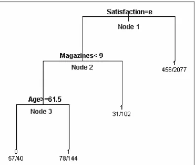
Figure 7: Classification tree for OWTP-dummy, obtained by rpart

The most important variable to determine whether anglers are willing to pay more or not, is the satisfaction of the anglers. If he anglers are not completely unsatisfied, they are most

Results and interpretation 20 likely willing to pay. The expenditure on magazines can further subdivide the anglers that are completely unsatisfied. If they spend at least 9 euro on magazines, then they are most likely willing to pay. If they are spending less than 9 euro, then age determines the willingness to pay: if the anglers are at least 61.5 years old, there are not willing to pay, else they are willing.

4.4.2 K-child decision trees Angling type

The k-child decision tree obtained by the macro TREEDISC is displayed in figure A2 (Appendix E2). The first splitting rule is the same rule as obtained by the binary classification tree, namely the fact whether an angler takes his fish home or not. Missing values for this variable are all send in the direction of the anglers who do take fish home.

The anglers that do not take their fish home are further subdivided according to age. The tree is not further subdivided into two groups as in the rpart-tree, but into three groups, namely the age-group 14-27, age-group 28-39 and the age-group 40 and older. Those anglers that have a missing value for age, were sent into the direction of the oldest group. The youngest age-group is then further subdivided according to the cost of the fishing equipment. The anglers that dominate the two lowest cost groups are the coarse fishers. The two highest cost groups are dominated by the carp anglers.

The age-group 28-39 is also further subdivided by the cost of the equipment. The lower cost group is dominated by the coarse anglers. The higher cost group (equipment costs more at least 1600 euro) is dominated by the carp anglers. The age-group of 40 year old and older anglers can be further subdivided according to their association need: the first group are the anglers that are already member of fishing club, the second group are the anglers that want to become member, or are not a member and have no desire to be come a member. In both obtained subgroups the coarse anglers dominate. Do note however that in the group that contains the anglers that are member of a fishing association, a lot of match anglers are present.

The anglers that take their fish home can be subdivided in the same way as with the r-part regression tree, namely by angling satisfaction. Note that the missing values for this variable

Results and interpretation 21 are all send in the way of the most satisfied. The anglers that are completely not satisfied are dominated by the predator fishers. Note that also the eel fishers are well represented in this group. The anglers that are not complete unsatisfied can further be subdivided according the degree of association they like. Coarse fishers dominate these two subgroups.

Only three of the seven angling types dominate an endnote. This is similar to the binary classification tree obtained by rpart. Also here the eel and predator fishers are mostly represented in the subtree of the anglers that take their fish back home.

Overall willingness to pay – dummy

Figure A3 (Appendix E2) shows the CHAID decision three for the OWTP-dummy variable. The first splitting rule is the same rule as the classification rule of rpart, namely the angler’s satisfaction. The group of the completely unsatisfied can be further subdivided into a group that spends more than 10 euro on magazines and into a group that spends less.

The group of the more satisfied can be further subdivided depending on the expenditure for the fishing equipment. The anglers that have spent between 400 and 2000 euro for their fishing gear can be further subdivided according to profession. The anglers that have spent at least 2000 euro, can be split into the group that takes fish home, and the group that does not.

When the angler is complete unsatisfied, the proportion of anglers that is not willing to pay is about 42,3% if the angler spends 10 euro or more on magazines and this proportion is 30,4% if the angler spends less. There can be seen relationship between the expenditure on equipment and the proportion of people that are not willing to pay: the more the angler spends on his equipment, the smaller the proportion of people that are not willing to pay.

4.5 Zero inflated poisson regression

( )

( )

Results and interpretation 22 where

1

X is the expenditure on magazines, X₂the age of the angler,X₃andX₄dummy variables for the membership status (reference category is always set as the last category),X₅,X₆,X₇,X₈

dummy variables for the angler’s satisfaction,X₉the expenditure on fishing equipment,X₁₀

the number of fishing trips a year,X₁₁ distance to the fishing spot,X₁₂,X₁₃,X₁₄,X₁₅,X₁₆

dummy variables for the angler’s salary.

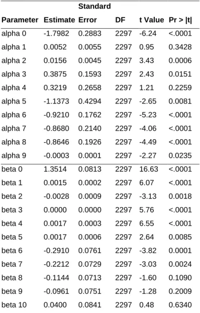
The following table shows the parameter estimates for the model. Note that αˆ₁ was not significant, but had to remain in the model, because the interaction effect between magazine expenditure and age was significant.

Table 6: Parameter estimates of the zero inflated poisson regression model

Standard

Parameter Estimate Error DF t Value Pr > |t| alpha 0 -1.7982 0.2883 2297 -6.24 <.0001 alpha 1 0.0052 0.0055 2297 0.95 0.3428 alpha 2 0.0156 0.0045 2297 3.43 0.0006 alpha 3 0.3875 0.1593 2297 2.43 0.0151 alpha 4 0.3219 0.2658 2297 1.21 0.2259 alpha 5 -1.1373 0.4294 2297 -2.65 0.0081 alpha 6 -0.9210 0.1762 2297 -5.23 <.0001 alpha 7 -0.8680 0.2140 2297 -4.06 <.0001 alpha 8 -0.8646 0.1926 2297 -4.49 <.0001 alpha 9 -0.0003 0.0001 2297 -2.27 0.0235 beta 0 1.3514 0.0813 2297 16.63 <.0001 beta 1 0.0015 0.0002 2297 6.07 <.0001 beta 2 -0.0028 0.0009 2297 -3.13 0.0018 beta 3 0.0000 0.0000 2297 5.76 <.0001 beta 4 0.0017 0.0003 2297 6.55 <.0001 beta 5 0.0017 0.0006 2297 2.64 0.0085 beta 6 -0.2910 0.0761 2297 -3.82 0.0001 beta 7 -0.2212 0.0729 2297 -3.03 0.0024 beta 8 -0.1144 0.0713 2297 -1.60 0.1090 beta 9 -0.0961 0.0751 2297 -1.28 0.2009 beta 10 0.0400 0.0841 2297 0.48 0.6340

Results and interpretation 23 When certain variables are used to predict bothp andλ it can be difficult to interpret the

overall effect when the estimates have the same sign. The difficulty does not occur in the model (αˆ₁has the same sign asβˆ₁, butαˆ₁ is not significant).When interpreting the parameter estimates, there can be concluded that the older the angler is, the bigger the probability that he is not willing to pay, and the lower the willingness to pay. The overall effect of the membership status is not clear, but the anglers that are not in an angling association have a bigger probability of not willing to pay than those who are. The less satisfied the angler is, the higher the probability of not willing to pay. The bigger the interaction effect of age and magazines expenditure is, the smaller the probability of not willing to pay.

The more anglers spend on magazines, the more they are willing to pay. The same counts for expenditure on fish equipment. The longer the distance the angler has to cover to his favourite fishing spot, the more he is willing to pay. The same effect counts for the number of times the angler goes each year on a fishing trip. The overall effect for the angler’s salary is difficult to interpret, but the anglers that have the lowest wages are willing to pay less than the ones that have the largest wages.

It is also important to mention that 694 of the 2991 observations were not used because of missing data.

Discussion 24

5. Discussion

A first important fact to discuss is the non-response in the original survey. Non-response in mail surveys is not a problem in itself, but non-response can induces a bias in the estimates, because non-respondents usually differ in important characteristics from respondents. A good approach to tackle this non-response could be the conduction of telephone follow-up survey to estimate the non-response bias6.

It is also essential to acknowledge response errors. Some questions could be misinterpret, or anglers could try to deceive the researchers, as they for instance could give lower values to their willingness to pay, in an attempt to influence the policy makers to their benefit6.

In order to get more insight into the profile of the Flemish angler, some extra questions could be added to the survey. One could look for instance at which fishing gear the anglers use or at which motivations the anglers have to go fishing34. Possible motives could be the satisfaction of other needs at the waterside, catching fish for consumption, just catching fish or the relaxation and enjoyment of the nature35.

It is important to acknowledge the fact that if model output corresponds to collected data, it does not necessarily mean that it will correspond in the future36. The dynamic character of human behaviour may not be neglected.

A framework for fisheries policy 25

6. A framework for fisheries policy

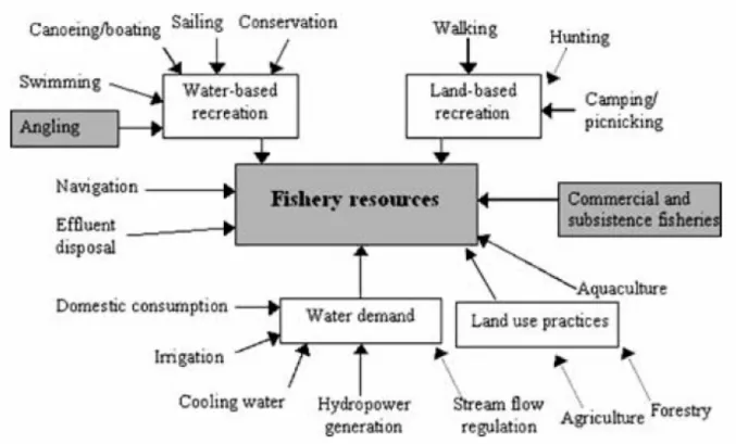
Failure to understand the users of fisheries resources and the dynamics of the behavior of these users will limit the success of policy decisions36. A key element for sustainable inland fisheries management is inclusion of all stakeholders. This will assure that decisions will better reflect social, economic and environmental conditions37. The follow picture points out the different stakeholders that interplay with inland fisheries management.

Figure 8: Stakeholders that typically affect fisheries and fishery resources in inland waters (source: Arlinghaus3 et al. 2002)

In the development of a decent management policy, consideration must be given to the preferences of the stakeholders within the system, especially when a large number and diverse range of interest groups exists38.

Some, or all of the groups that are involved in the management process, may have conflicting objective preferences towards management direction. Therefore, it is highly relevant to evaluate stakeholder preferences for inclusion in the decision-making process. This enables

A framework for fisheries policy 26

the policy makers to justify decisions, based on importances and priorities expressed by stakeholders, more explicitly. Generally in natural resource management cases, objectives are categorized under three main headings: environmental (e.g. biological and conservational), economic and social objectives38.

Mardle et al. (2004) suggested that the analytic hierarchy process (AHP) can be used to develop importance structures between criteria and/or potential policy for the analysis of management problems. The key feature of this approach is that value judgments are incorporated in the process, giving those with an interest in management the opportunity to explicitly state their preferences with respect to the identified objectives38.

A problem with the AHP approach is that it is not a valid multi-criteria method. Different authors, for example Barzilai39,40 (2005,2001) and Bana e Costa41 et al. (2001), have shown essential flaws in the AHP. A solution is to use another multi-criteria method.

ARGUS (achieving respect for grades by using ordinal scales only) is a multi-criteria method based on the general idea of outranking. It avoids the pitfall of treating a criterion, with evaluations on an ordinal scale, as a criterion with evaluations on an interval or ratio scale by forcing the decision maker to indicate the scale of measurement for each criterion. It gives the decision maker the opportunity of taking, for criteria with evaluations on a ratio scale, the order of magnitude of the evaluations into account when modeling his preference structure. The method assumes that the importance of the criteria must be measured on an ordinal scale, and does not always end with only one good alternative but with a set of good alternatives42.

A schematic overview of the proposed framework is given in the figure 9. The different possible policy actions (alternatives) are determined by the complete group. The criteria and the evaluations on the criteria can be determined in the group (environmental, economic or social) or by the individual in the group. Each decision maker can then use its own data such as preferences, importances of criteria and evaluations on the criteria, as input for the multi-criteria-method he prefers, e.g. ARGUS. The individual rankings then can be combined to a group ranking, and this group ranking can on its turn be combined into a final ranking.

A framework for fisheries policy 27

Figure 9: A framework for fisheries policy

De Keyser et al (2002) described how the individual rankings can be combined into a group ranking. A good measure of how well a ranking fits another ranking is the rank correlation coefficient of Kendall, corrected for ties43.

In order to improve policy decisions the stakeholder views must be identified and understood, and a compromise must be sought between competing and conflicting demands. An improved communication between the policy makers and the stakeholders is thus of essential importance for the sustainability of the fisheries resources3.

DM1 DM2 … DMP1 DM1 DM2 … DMP3 DM: decision maker MCM: multi-criteria method IR: individual ranking

MR

IR

Entire Group Ranking Entire group of decision makers Decision problem: alternatives

Environmental decision makers Economic decision makers Social decision makers Decision problem:

criteria and evaluations

Decision problem: criteria and evaluations

Decision problem: criteria and evaluations

DM1 DM2 … DMP2 MR IR MR IR MR IR MR IR MR IR MR IR MR IR MR IR Environmental Group Ranking Economic Group Ranking Social Group ranking

Conclusion 28

7. Conclusion

The results of the binary decision trees, k-child decision trees and the zero-inflated poisson were similar, but it is important to stress that decision trees can handle missing values fairly easily.

When different types of anglers were compared, it could be seen that there was a clear separation between eel and predator anglers on the one side, and the other types of anglers on the other site. This difference was also highlighted by the discriminant analysis and could be explained by the fact whether an angler takes the fish home or not. The catch-and release anglers are thus clearly different from anglers who fish to consume.

When the emphasis is laid on finding differences in angling satisfaction, the difference between eel and predator anglers on the one hand, and the other types of anglers on the other hand, pops up again. The eel and predator anglers are clearly less satisfied than the other anglers.

The overall willingness to pay is generally higher when anglers spend more money on their fishing equipment and on magazines. It is highest for carp anglers. This is also established in German studies35.

A key point for an efficient fisheries policy is to understand the preferences of all stakeholders. In the previous chapter a framework was presented to take different, and sometimes conflicting, opinions into account. A policy will only be successful if all stakeholders are willing to participate.

References 29

References

[1] Ditton, R.B., Hunt, K.M. (2001). Combining creel intercept and mail survey methods to understand the human dimensions of local freshwater fisheries, Fisheries management

and ecology, 8, p.295-301

[2] Vandenabeele, P. (1987). De hengelaar in het Vlaamse Gewest, Groenendaal-Hoeilaart: Rijksstation voor bos-en hydrobiologisch onderzoek

[3] Robert Arlinghaus, R., Mehner, T., Cowx, G. (2002). Reconciling traditional inland fisheries management and sustainability in industrialized countries, with emphasis on Europe, Fish and fisheries, 3, p. 261 -316

[4] Peirson, G., Tingley, D., Spurgeon, J., Radford, A. (2001). Economic evaluation of inland fisheries in England and Wales, Fisheries management and ecology, 8, p.415-424 [5] Toivonen, A.-L., Roth, E., Navrud, S., Gudbergsson, G., Appelblad, H., Bengtsson, B., Tuunainen, P. (2004). The economic value of recreational fisheries in Nordic countries,

Fisheries management and ecology, 11, p.1-14

[6] Pollock, K.H., Jones, C.M., Brown, T.L. (1994). Angler survey methods and their

applications in fisheries management, Maryland: American fisheries society.

[7] Navrud, S. (2001). Economic valuation of inland recreational fisheries: empirical studies and their policy use in Norway, Fisheries management and ecology, 8, p.369-382

[8] Coussement, M. (2002). De grote V.V.H.V. hengelsport-enquête, Het VVHV

hengelblad, jaargang 11, nr. 6, p.11-19

[9] Dumortier M, De Bruyn L, Peymen J, Schneiders A, Van Daele T, Weyemberh G, van Straaten D & Kuijken E (2003) Natuurrapport 2003. Toestand van de natuur in Vlaanderen: cijfers voor het beleid. Mededelingen van het Instituut voor Natuurbehoud, nr. 21, Brussel.

[10] Dumortier M, De Bruyn L, Hens M, Peymen J, Schneiders A, Van Daele T, Van Reeth W, Weyemberh G & Kuijken E (2005) Natuurrapport 2005. Toestand van de natuur in Vlaanderen: cijfers voor het beleid. Mededelingen van het Instituut voor Natuurbehoud ,nr. 24, Brussel.

[11] Vandecruys, W. (2004). Economische en sociale aspecten van de hengelsport op

openbaar water in Vlaanderen, Diepenbeek : LUC.

[12] Govarts, E. (2004). Profile and economic evaluation of angling on public angling

waters in Flanders, Diepenbeek: LUC

[13] Arlinghaus, R., Mehner, T. (2004). Testing the reliability and construct validity of a simple and inexpensive procedure to measure the use value of recreational fishing,

Fisheries management and ecology, 11, p.61-64

[14] Fernandez, G. (2003). Data mining using SAS applications, Boca Raton: Chapman & Hall/CRC

[15] Hair, J.F., Anderson, R.E., Tatham, R.L., Black, W.C. (1998). Multivariate data

References 30 [16] Johnson, R.A., Wichern, D.W. (2002) Applied multivariate statistical analysis, Upper

Saddle River: Prentcie-Hall

[17] MacQueen, J.B. (1967). Some methods for classification and analysis of multivariate observations, proceedings of 5th Berkeley symposium on mathematical statistics and

probability, 1, Berkeley: University of California Press, p.281-297

[18] Scherer, W.T., Smith, B.L. ,Hauser, T.A. (2001). Data Mining Tools for the Support of

Traffic Signal Timing Plan Development in Arterial Networks, Charlottesville: Center

for Transportation Studies - University of Virginia.

Online available at: http://www.gmupolicy.net/its/papers2/paper-Smith-AdaptiveSignalsDecisionSupportSystem.pdf

[19] SAS Institute Inc. 2004. (2004). SAS/STAT® 9.1 User’s Guide. Cary, NC: SAS Institute Inc.

[20] Molenberghs, G., Geys, H. (2004). Course notes multivariate data analysis, Diepenbeek: LUC.

[21] Arentze, T., Katoshevski, R., Timmermans, H. (2001). A micro-simulation model of

activity-travel behaviour of individuals in urban environments, Eindhoven: Urban

Planning Group – Eindhoven University of Technology

[22] Mesa, D.M., Tsai, P., Chambers, R.L. (2000). Using tree-based models for missing data

imputation: an evaluation using UK census data, Southampton: University of

Southampton.

Online available: http://www.cbs.nl/en/service/autimp/Tree-(AUTIMP).pdf

[23] Breiman, L., Friedman, J.H., Olshen, R.A., Stone, C.J. (1984). Classification and

regression trees, Belmont: Wadsworth

[24] SPSS Inc. (1999). SPSS white paper: AnswerTree algorithm summary -

ATALGWP-0599, SPSS Inc.

Online available: http://bus.utk.edu/stat/datamining/ATALGWP-0599.pdf

[25] Therneau, T.M., Atkinson, E.J. (1997). An Introduction to Recursive Partitioning Using

the RPART Routines, Jacksonville: Mayo Foundation

Online available: http://www.mayo.edu/hsr/techrpt/61.pdf

[26] McLachlan, G. J. (1992). Discriminant Analysis and Statistical Pattern Recognition, New York:Wiley

[27] The R Development Core Team , (2005). R: A Language and Environment for

Statistical Computing : Reference Index, R Foundation for Statistical Computing

[28] Eherler, D., Lehmann, T. (2001). Responder profiling with CHAID and dependency

analysis, Jena: Friedrich-Schiller-University

Online available: http://www.informatik.uni-freiburg.de/~ml/ecmlpkdd/WS-Proceedings/w10/lehmann.pdf

[29] Kass, G.V. (1980). An exploratory technique for investigating large quantities of categorical data, Journal of the royal statistical society (series c), vol. 29, no.2, p.119-127

[30] Anonymous (1995) Treedisc Macro - Beta version: CHAID-like Classification Trees Online available: http://www.stat.lsu.edu/faculty/moser/exst7037/treedisc.html

References 31 [31] Lambert, D. (1992). Zero-inflated poisson regression with an application to defects in

manufacturing, Technometrics, vol. 34, no.1, p.1-14

[32] Lee, A.H., Wang, K., Yau, K.K.W. (2001). Analysis of zero-inflated poisson data incorporating extent of exposure, biometrical journal, 43, 8, p.963-975

[33] Stratford, J.A. (2005). Dealing with the zero problem in ecological data, Auburn: Auburn University. Online available: http://www.auburn.edu/~stratja/zeros.htm

[34] Wedekind, H., Hilge, V., Steffens, W. (2001). Present status, and social and economic significance of inland fisheries in Germany, Fisheries Management and Ecology, vol. 8, nr. 4-5, p. 405-414

[35] Arlinghaus, R., Mehner, T. (2002). Socio-economic characterisation of specialised common carp (Cyprinus carpio L.) anglers in Germany, and implications for inland fisheries management and eutrophication control, Fisheries Research, 1475, p.1-15. [36] Radomski, P.J., Goeman, T.J.(1996). Decision making and modelling in freshwater

sport-fisheries management, Fisheries, Vol.21, No. 12, p.14-21

[37] Sipponen, M., Gréboval, D. (2001). Social, economic and cultural perspectives of European inland fisheries: review of the EIFAC symposium on fisheries and society,

Fisheries management and ecology, 8, p.283-293

[38] Mardle, S., Pascoe, S., Herro, I. (2004). Management objective importance in fisheries: an evaluation using the analytic hierarchy process (AHP), Environmental management, vol.33, no.1, p.1-11

[39] Barzilai, J. (2005). Measurement and preference function modelling, International

transactions in operational research, 12, p.173–183

[40] Barzilai, J. (2001). Notes on the analytic hierarchy process, Proceedings of the NSF

Design and manufacturing research conference, Tampa, p.1-6

[41] Bana e Costa, C.A., Vansnick, J.-C. (2001). A fundamental criticism to Saaty's use of

the eigenvalue procedure to derive priorities, Working Paper LSE OR 01.42, London

School of Economics

[42] De Keyser, W., Peeters, P. (1994). ARGUS - a new multiple criteria method based on the general idea of outranking, EUROCOURSES: Environmental Management. Dordrecht: Kluwer Academic Publishers, vol. 3, pp. 263–278.

[43] De Keyser, W., Springael, J. Johan. (2002). Another way of looking at group decision making opens new perspectives, Antwerpen: UFSIA

Appendix 32

Appendix

A. SAS Code for the zero-inflated poisson regression

data YOURDATA;

infile 'YOURFILE’ dlm =',' firstobs=2; input YOURVARS;

run;

/* this genmod procedure estimates the response without zero-inflation and without covariates */

proc genmod data=yourdata;

model RESPONSE = /link=log dist=poisson; run;

/* the nlmixed procedure models a degenerate zero and a Poisson distribution; the end product giving you a probability of an observation being in the zero distribution */ proc nlmixed data=YOURDATA;

/* a0 = intercept of the logistic model of the inflation prob, a1 is that slope, b0-b1 are the regression coefficients for the Poisson mean */

parameters a0=0 a1=0 a2=0 a3=0 b0=0 b1=0 b2=0; /* linear predictor for the inflation probability */ linpinfl = a0 + a1*VAR1 + a2*VAR2 + a3*VAR1*VAR2; /* infprob = inflation probability for zeros */ /* = logistic transform of the linear predictor */ infprob = 1/(1+exp(-linpinfl));

/* Poisson mean */

lambda = exp(b0 + b1*VAR1 +b2*VAR2); /* Build the ZIP log likelihood */

if response=0 then

ll = log(infprob + (1-infprob)*exp(-lambda));

else ll = log((1-infprob)) + RESPONSE*log(lambda) - lgamma(response+1) - lambda; model RESPONSE ~ general(ll);

/* predict statement to get the predicted number of RESPONSES given the Poisson mean and the inflation probability */

predict (1-infprob)*lambda out = PREDICTED_RESPONSE; run;

Appendix 33

B. Results EDA for the different angling types

B1. Frequency tables for the different predictor variables × angling type Table A1: Frequency table of profession × angling type

Coarse fishing Carp fishing Fly fishing Boat fishing Match fishing Eel fishing Predator fishing Total

Student 120 (41,96%) 104 (36,36%) 1 (0,35%) 0 (0,00%) 10 (3,50%) 19 (6,64%) 32 (11,19%) 286 (100%) Workman 507 (45,76%) 255 (23,01%) 5 (0,45%) 8 (0,72%) 102 (9,21%) 87 (7,85%) 144 (13,00%) 1108 (100%) Employee 240 (55,43%) 63 (14,55%) 7 (1,62%) 4 (0,92%) 32 (7,39%) 25 (5,77%) 62 (14,32%) 433 (100%) Executive 92 (57,50%) 24 (15,00%) 5 (3,13%) 1 (0,63%) 6 (3,75%) 7 (4,38%) 25 (15,63%) 160 (100%) Retired 486 (63,12%) 47 (6,10%) 4 (0,52%) 8 (1,04%) 30 (3,90%) 89 (11,56%) 106 (13,77%) 770 (100%) Unemployed 85 (49,13%) 28 (16,18%) 0 (0,00%) 2 (1,16%) 5 (2,89%) 20 (11,56%) 33 (19,08%) 173 (100%)

Table A2: Frequency table of age class × angling type

Coarse fishing Carp fishing Fly fishing Boat fishing Match fishing Eel fishing Predator fishing Total

Age 14-35 323 (37,21%) 322 (37,10%) 4 (0,46%) 3 (0,35%) 53 (6,11%) 57 (6,57%) 106 (12,21%) 868 (100%) Age 36-64 914 (57,96%) 159 (10,08%) 16 (1,01%) 17 (1,08%) 113 (7,17%) 129 (8,18%) 229 (14,51%) 1577 (100%) Age 65-90 264 (64,08%) 26 (6,31%) 2 (0,49%) 4 (0,97%) 16 (3,88%) 46 (11,17%) 54 (13,11%) 412 (100%)

Table A3: Frequency table of years of experience (y.o.e.) × angling type

Coarse fishing Carp fishing Fly fishing Boat fishing Match Eel fishing Predator Total

0-10 y.o.e. 299 (46,21%) 191 (29,52%) 2 (0,31%) 2 (0,31%) 26 (4,02%) 54 (8,35%) 73 (11,28%) 647 (100%) 11-20j y.o.e. 268 (44,22%) 161 (26,57%) 4 (0,66%) 6 (0,99%) 41 (6,77%) 53 (8,75%) 73 (12,05%) 606 (100%) 21-30j y.o.e. 263 (51,27%) 84 (16,37%) 6 (1,17%) 3 (0,58%) 42 (8,19%) 33 (6,43%) 82 (15,98%) 513 (100%) 31-40j y.o.e. 339 (58,65%) 56 (9,69%) 5 (0,87%) 7 (1,21%) 50 (8,65%) 43 (7,44%) 78 (13,49%) 578 (100%) 41-50j y.o.e. 179 (59,67%) 22 (7,33%) 4 (1,33%) 1 (0,33%) 16 (5,33%) 28 (9,33%) 50 (16,67%) 300 (100%) >50j y.o.e. 200 (64,10%) 10 (3,21%) 1 (0,32%) 5 (1,60%) 12 (3,85%) 35 (11,22%) 49 (15,71%) 312 (100%)

Appendix 34 Table A4: Frequency table of angling type × harvest (take fish home)

Harvest (No) Harvest (Yes) Total Coarse fishing 1274 (82,83%) 264 (17,17%) 1538 (100%) Carp fishing 474 (91,33%) 45 (8,67%) 519 (100%) Fly fishing 16 (72,73%) 6 (27,27%) 22 (100% Boat fishing 8 (40,00%) 12 (60,00%) 20 (100%) Match fishing 169 (91,85%) 15 (8,15%) 184 (100%) Eel fishing 69 (28,05%) 177 (71,95%) 246 (100%) Predator fishing 130 (32,26%) 273 (67,74%) 403 (100%) Table A5: Frequency table of angling type × angling satisfaction

satis 1 satis 2 satis 3 satis 4 satis 5 Total Coarse fishing 60 (3,85%) 660 (42,33%) 282 (18,09%) 353 (22,64%) 204 (13,09%) 1559 (100%) Carp fishing 29 (5,56%) 191 (36,59%) 114 (21,84%) 147 (28,16%) 41 (7,85%) 522 (100%) Fly fishing 0 (0,00%) 9 (40,91%) 4 (18,18%) 6 (27,27%) 3 (13,64%) 22 (100%) Boat fishing 0 (0,00%) 9 (37,50%) 4 (16,67%) 9 (37,50%) 2 (8,33%) 24 (100%) Match fishing 8 (4,28%) 68 (36,36%) 32 (17,11%) 57 (30,48%) 22 (11,76%) 187 (100%) Eel fishing 2 (0,81%) 67 (27,02%) 37 (14,92%) 68 (27,42%) 74 (29,84%) 248 (100%) Predator fishing 10 (2,47%) 116 (28,64%) 64 (15,80%) 111 (27,41%) 104 (25,68%) 405 (100%) satis 1 = complete satisfied satis 2 = satisfied satis 3 = neutral

satis 4 = not satisfied satis 5 = completely not satisfied Table A6: Frequency table of angling type × cost of fishing trip

0-5€ 6-10€ 11-20€ 20+€ Total Coarse fishing 608 (39,90%) 494 (32,41%) 291 (19,09%) 131 (8,60%) 1524 (100%) Carp fishing 92 (17,83%) 153 (29,65%) 159 (30,81%) 112 (21,71% 516 (100%) Fly fishing 7 (33,33%) 6 (28,57%) 1 (4,76%) 7 (33,33%) 21 (100%) Boat fishing 3 (13,04%) 4 (17,39%) 6 (26,09%) 10 (43,48%) 23 (100%) Match fishing 13 (7,03% 36 (19,46%) 61 (32,97%) 75 (40,54%) 185 (100%) Eel fishing 128 (55,17%) 64 (27,59%) 22 (9,48%) 18 (7,76%) 232 (100%) Predator fishing 166 (43,12%) 131 (34,03%) 60 (15,58%) 28 (7,27%) 385 (100%) Table A7: Frequency table of angling type × cost of fishing equipment

0-250€ 251-1000€ 1001-2000€ 2000+€ Total Coarse fishing 383 (26,30%) 688 (47,25%) 230 (15,80%) 155 (10,65%) 1456 (100%) Carp fishing 77 (15,52%) 148 (29,84%) 110 (22,18%) 161 (32,46%) 496 (100%) Fly fishing 0 (0,00%) 9 (42,86%) 4 (19,05%) 8 (38,10%) 21 (100%) Boat fishing 2 (9,09%) 6 (27,27%) 3 (13,64%) 11 (50,00%) 22 (100%) Match fishing 10 (5,56%) 35 (19,44%) 46 (25,56%) 89 (49,44%) 180 (100%) Eel fishing 111 (47,84%) 88 (37,93%) 20 (8,62%) 13 (5,60%) 232 (100%) Predator fishing 111 (28,83%) 173 (44,94%) 46 (11,95%) 55 (14,29%) 385 (100%) Table A8: Frequency table of angling type × expenditure on magazines

0 € 1-40 € 40+ € Total Coarse fishing 1073 (68,96%) 279 (17,93%) 204 (13,11%) 1556 (100%) Carp fishing 253 (48,37%) 102 (19,50%) 168 (32,12%) 523 (100%) Fly fishing 2 (9,09%) 9 (40,91%) 11 (50,00%) 22 (100%) Boat fishing 16 (66,67%) 3 (12,50%) 5 (20,83%) 24 (100% Match fishing 89 (47,59%) 56 (29,95%) 42 (22,46%) 187 (100%) Eel fishing 195 (79,59%) 32 (13,06%) 18 (7,35%) 245 (100%) Predator fishing 265 (65,59%) 76 (18,81%) 63 (15,59%) 404 (100%)

Appendix 35 Table A9: Frequency table of angling type × membership status

Membership 1 Membership 2 Membership 3 Total Coarse fishing 982 (63,77%) 118 (7,66%) 440 (28,57%) 1540 (100%) Carp fishing 278 (53,36%) 47 (9,02%) 196 (37,62%) 521 (100%) Fly fishing 5 (22,73%) 2 (9,09%) 15 (68,18%) 22 (100%) Boat fishing 11 (45,83%) 1 (4,17%) 12 (50,00%) 24 (100%) Match fishing 19 (10,16%) 2 (1,07%) 166 (88,77% 187 (100%) Eel fishing 184 (76,03%) 20 (8,26%) 38 (15,70%) 242 (100%) Predator fishing 255 (63,28%) 41 (10,17%) 107 (26,55%) 403 (100%) Membership 1 = angler does not want to be member of a fishing association

Membership 2 = angler considers to become a member of a fishing association in the future Membership 3 = angler is member of a fishing association

B2. Descriptive statistics for the different continuous variables

Table A10: Basic measures of central tendency for the variable “frequency of fishing”

Mean Standard error 5% Trimmed mean Standard error Median Coarse fishing 34.07 1.10 28.05 0.82 20.00 Carp fishing 44.12 2.16 37.79 1.94 30.00 Fly fishing 18.67 4.08 15.65 3.80 10.00 Boat fishing 45.54 14.65 31.10 4.79 30.00 Match fishing 48.18 3.10 43.96 2.41 40.00 Eel fishing 41.51 3.66 33.22 3.04 20.00 Predator fishing 43.84 2.90 34.94 2.25 25.00 Total 38.60 0.89 31.86 0.69 24.00

Table A11: Basic measures of central tendency for the variable “cost fishing trip”

Table A12: Basic measures of central tendency for the variable “cost fishing equipment”

Mean Standard error 5% Trimmed mean Standard error Median Coarse fishing 1011.16 46.33 814.76 23.74 500.00 Carp fishing 2008.52 109.64 1666.52 81.42 1300.00 Fly fishing 2713.10 672.07 2100.00 492.91 2000.00 Boat fishing 3215.91 861.45 2383.33 818.35 2150.00 Match fishing 2722.94 225.60 2317.51 150.42 2000.00 Eel fishing 820.85 143.15 495.81 46.16 300.00 Predator fishing 1098.10 88.60 842.00 51.69 500.00 Total 1321.03 40.41 1022.27 24.17 619.50 Mean Standard error 5% Trimmed mean Standard error Median Coarse fishing 10.23 0.23 9.26 0.19 10.00 Carp fishing 17.04 0.63 15.62 0.63 12.00 Fly fishing 15.67 3.25 14.06 3.72 10.00 Boat fishing 19.85 2.66 18.58 2.24 20.00 Match fishing 20.62 0.91 19.75 0.91 20.00 Eel fishing 8.59 0.61 7.39 0.50 5.00 Predator fishing 10.20 0.53 8.75 0.37 10.00 Total 12.06 0.21 10.68 0.17 10.00