régression et les modèles structurels en présence
d’hétéroscédasticité de forme arbitraire
Par
Elise Coudin
Thèse de doctorat effectuée en cotutelle au
Département de Sciences économiques Faculté des arts et des sciences
et à
l’Ecole des Hautes Etudes en Sciences Sociales
Thèse présentée à la Faculté des études supérieures en vue de l’obtention du grade de Philosophiae Doctor (Ph.D.)
en sciences économiques et à
l’Ecole des Hautes Etudes en Sciences Sociales envue de l’obtention du grade de Docteur
Juin2007
• -J
t-çi
o
Université
dl1
de Montréal
Directiondes bibliothèques
AVIS
L’auteur e autorisé l’Université de Montréal à reproduire et diffuser, en totalité ou en partie, par quelque moyen que ce soit et sur quelque support que ce soit, et exclusivement à des fins non lucratives d’enseignement et de recherche, des copies de ce mémoire ou de cette thèse.
L’auteur et les coauteurs le cas échéant conservent la propriété du droit d’auteur et des droits moraux qui protègent ce document. Ni la thèse ou le mémoire,
ni
des extraits substantiels de ce document, ne doivent être imprimés ou autrement reproduits sans l’autorisation de l’auteur.Afin de se conformer à la Loi canadienne sur la protection des renseignements personnels, quelques formulaires secondaires, coordonnées ou signatures intégrées au texte ont pu être enlevés de ce document. Bien que cela ait pu affecter la pagination, il n’y a aucun contenu manquant. NOTICE
The author of this thesis or dissertation has granted a nonexclusive license allowing Université de Montréal to reproduce and publish the document, in part or in whole, and in any format, solely for noncommercial educational and research purposes.
The author and co-authors if applicable retain copyright ownership and moral rights in this document. Neither the whole thesis or dissertation, nor substantial extracts from it, may be printed or otherwise reproduced without the author’s permission.
In compliance with the Canadian Privacy Act some supporting forms, contact information or signatures may have been removed from the document. While thîs may affect the document page count, it does flot represent any Ioss of content from the document.
Université de Montréal Faculté des études supérieures
et
Ecole des Hautes Etudes en Sciences Sociales
Cette thèse intitulée
Inférence exacte et non-paramétrique dans les modèles de
régression et les modèles structurels en présence
d’hétéroscédasticité de forme arbitraire
Présentée et soutenue à l’Université de Montréal par:Elise Coudin
a été évaluée par un jury composé des personnes suivantes:
Président-rapporteur et membre du jury
L-Directeur de recherche (Université de Montréal) Directeur de recherche (EHESS) Examinateurs externes3-..t[.n
Membres du jury.t.t
Représentant du doyen delafESL’objet de cette thèse est de développer un système d’inférence exacte en échantillon fini dans des modèles de régression et des modèles structurels sans imposer d’hypothèse paramétrique sur la distribution des erreurs.
Dans le premier essai, nous étudions la construction de tests et de régions de confiance dans une régression linéaire sur la médiane. Le modèle que nous considérons n’impose pas de restriction paramétrique sur la distribution des erreurs. Celles-ci peuvent être non gaus siennes, hétéroscédastiques ou bien présenter une dépendance sérielle de forme arbitraire. Habituellement, l’analyse de ce type de modèle a recours à des approximations asympto tiques normales, lesquelles peuvent être trompeuses en échantillon fini. Nous introduisons une propriété analogue à la différence de martingale pour la médiane, la « mediangale », et remarquons que les signes d’une suite de « mediangale » sont indépendants entre
eux et suivent une distribution connue et simulable. Nous utilisons alors la transforma
tion par les signes et proposons des statistiques pivotales qui, en plus d’être robustes, per mettent de construire une approche d’inférence simultanée valide quelle que soit la taille de l’échantillon. Grâce à la méthode des tests de Monte Carlo et à celle des projections, nous construisons tour à tour des tests et des régions de confiance simultanés puis des tests et des régions de confiance pour n’importe quelle tranformation du paramètre. Nous fournissons ensuite une théorie asymptotique sous des hypothèses plus faibles que la « mediangale ». Les études par simulation montrent que la méthode proposée est plus performante que les méthodes asymptotiques habituelles lorsque le processus est très hétérogène ou lorsque la taille de l’échantillon est petite. Enfin, deux exemples d’application sont étudiés. Dans le premier, nous testons la présence d’une tendance sur des données financières. Le deuxième s’appuie sur des données régionales, nécéssairement peu nombreuses, pour tester la théorie macroéconomique de/3convergence entre les niveaux de production des états américains.
Dans le deuxième essai, nous introduisons un estimateur et des outils d’inférence va
lides en échantillon fini moins communément utilisés. Nous étudions, tout d’abord, la fonction p-value qui associe un degré de confiance à chaque valeur testée du paramètre étant donnée la réalisation de l’échantillon. Celle-ci est reliée à la notion de distribution de confiance et aux distributions fiducielles de Fisher [Fisher (1930)]. Ces outils fournissent
un équivalent fréquentiste aux distributions bayésiennes a
posteriori.
Nous calculons des fonctions p-value simulées à partir de tests de Monte Carlo simultanés, puis des versions projetées pour chaque composante individuelle du paramètre. Nous suivons ensuite le prin cipe d’inversion de test de Hodges et Lehmann [Hodges et Lebmann (1963)] et propo sons d’utiliser comme estimateur, la valeur du paramètre associée au plus haut degré de confiance (à la plus forte p-value). L’estimateur de signe qui en découle est sans biais pour la médiane quand les erreurs sont symétriques, et il partage les propriétés d’équivariance de l’estimateur des moindres valeurs absolues(«
Least Absolute Deviations, LAD >). Il est aussi convergent et asymptotiquement normal sous des conditions plus faibles que l’estima teur LAD. En échantillon fini, les simulations suggèrent qu’il est plus performant en termes de biais et d’erreur quadratique moyenne pour des processus très hétérogènes. Ces outils permettent de compléter l’analyse des deux exemples empiriques étudiés précédemment.Dans le troisième essai, nous développons une approche inférencielle exacte en échan tillon fini pour des modèles structurels non-linéaires. Nous proposons une version de la propriété de pivotalité des signes adaptée à un modèle instrumental. Les tests exacts qui en découlent ne dépendent pas du degré d’identification du paramètre. Ils sont en particulier valides en présence d’instruments faibles, pour des erreurs possiblement hétéroscédastiques et non gaussiennes. L’approche que nous proposons fait intervenir des régressions artifi cielles où l’on régresse les signes contraints sur des instruments auxiliaires dans l’esprit d’Anderson et Rubin [Anderson et Rubin (1949), Dufour (2003)]. Nous étudions de plus la question des instruments optimaux à inclure dans le modèle, ce qui permet de gagner de la puissance en cas de suridentification. Les simulations montrent que notre approche est plus performante que les méthodes usuelles (y compris celles qui sont robustes à la pré sence d’instruments faibles) lorsque les erreurs sont non gaussiennes, hétéroscédastiques et lorsque l’échantillon est petit. Cette méthode est utilisée sur les données de Angrist et Krueger (1991) pour analyser les rendements de l’éducation sur le salaire.
Mots clés : inférence exacte; régression sur la médiane régression quantile; test de signe; hétéroscédasticité; non nonnalité; dépendance; test de Monte Carlo; techniques de pro
jection; distribution de confiance; endogénéité; modèle structurel; modèle non-linéaire;
$ummary
The objective of this thesis is to develop a whote system of exact inference in fi nite samples, for regression models and structural econometric models under very weak distributional assumptions on the error term.
In the first essay, we study the construction of finite-sample distribution-free tests and confidence sets for the pararneters of a linear median regression when no parametric assumption is imposed on the noise distribution. The setup we consider allows for non normality, heteroskedasticity and nonlinear serial dependence of unknown forms. Such serniparametric models are usually analyzed using asymptotically justified approximate methods, which can be arbitrari]y unreliable in finite samples. We consider first the prop erty ofrnediangale—the median-based analogue ofa martingale difference
—and show that
the signs of mediangale sequences are distribution-free despite the presence of nonlinear dependence and heterogeneity of unknown form. We point out that a simultaneous infer ence approach in conjunction with sign transformations does provide statistics with the required pivotality features—in addition to usual robustness properties. Those sign-based
statistics are exploited— with Monte Carlo tests and projection techniques
— in order to
produce valid inference in finite samples: simultaneous tests, confidence regions and then more general projection-based tests are constructed. An asymptotic theory which holds under even weaker assumptions is also provided. Simulations suggest the good perfor mance of that method for a wide range of processes. Finally, two illustrative examples are presented. First, we test for the presence ofa drifi in financial series involving strong het eroskedasticity. Then, we exploit a cross-regional data set whose sample size is necessarily small, and test for /3 convergence between levels of per capita output across U.S. States.
The second essay presents additîonal finite-sample-based tools that can be used in con junction with the sign-based inference system previously developed. first, we study the p-value function which measures the confidence one may have in a certain value of the parameter. It is related to the notion of confidence distribution and to Fisher fiducial dis tributions [Fisher (1930)]. Those notions provide a frequentist analogue to the Bayesian posterior distributions. We combine sign-based Monte Carlo tests of simultaneous hy potheses with projection techniques to constmct simulated p-value functions and projected
versions for the parameter individual components. $ecotid, sign-based estimators that are the parameter values with the highest confidence (the highest p-value) are presented. These are obtained using the Hodges-Lehmann principle of test inversion [Hodges and Lehmann (1963)]. They are expected to present the same robustness properties than the test statistics from which they are derived and can directly be associated with the exact inference proce dures described inthe first essay. We atso show they are median unbiased (under a sym metry assumption) and present equivariance features similar to the LAD estimator. Consis tency and asymptotic normality are also provided under regularity conditions weaker than the ones required for the LAD estimator. In a simulation study ofbias and root mean square error (RMSE), we find that sign-based estimators perform better than the LAD estimator in settings with sizable heteroskedasticity. Sign-based estimators and p-value functions are then used to complete the analysis of the two practical examples studied previously.
The third essay devetops finite-sample distribution-free exact inference in nonlinear structural models. We propose an adapted version of the sign invariance that allows one to construct exact tests. We notice that the validity of those tests does not depend on identi fication assumptions nor onparametric approximations imposed onthe errors. Sign-based tests equal the nominal size for any given sample size in presence of weak instruments, with non-normal and heteroskedastic errors. Basically, the sign-based approach relies on artificiat regressions where the signs of the constrained residuats are regressed on some “auxiliary” instruments [Anderson and Rubin (1949), Dufour (2003)]. We also study the problem of building optimal instruments, which can lead to considerable gain of power in case of overidentification. Simulations show that sign-based methods overcome usual rnethods and methods robust to weak instruments in non-normal and heteroskedastic set tings. A re-analysis ofthe retums to education based on Angrist and Krueger (1991) data is also provided.
Key words: exact inference; median regression; quantile regression; sign test; het eroskedasticity; non-nonnality; dependence; Monte Carlo test; projection techniques; con fidence distribution; endogenenity; structural models; nonlinear models; instrument; weak instrument; consistency.
Table des matières
Sommaire
Summary ïii
Introduction 1
Chapitre 1 : Finite-sample distribution-free inference in linear median regres
sbus under heteroskedasticity and nonlinear dependence of unknown form 7
1. Introduction $
2. Framework 12
2.1. Model 12
2.2. Special cases 17
3. Exact finite-sampie sign-based inference 1$
3.1. Motivation 1$
3.2. Distribution-free pivotai functions and nonparametric tests 20
4. Regression sign-based tests 22
4. 1. Regression sign-based statistics 22
4.2. Monte Carlo tests 26
5. Regression sign-based confidence sets 28
5.1. Confidence sets and conservative confidence intervals 2$
5.2. Numerical illustration 30
6. Asymptotic theory 31
6.1. Asymptotic distributions oftest statistics 31
6.2. Asymptotic validity of Monte Carlo tests 32
6.2.2. Asymptotic validity of sign-based inference . 35 7. SimuLation study 36 7.1. Size 38 7.2. Power 41 7.3. Confidence intervals 45 8. Examples 47
8.1. Standard and Poor’s drift 47
8.2. /3-convergence across 1.3.5. States 50
9. Conclusion 52
A. Proofs 54
A.1. Proofof Proposition 2.5 54
A.2. Proof of Proposition 3.2 54
A.3. Proofof Proposition 3.3 55
A.4. Proof of Proposition 4.1 55
A.5. ProofofTheorem 6.1 58
A.6. ProofofCorollary 6.2 59
A.7. ProofofTheorem 6.3 59
A.8. ProofofTheorem 6.4 62
B. Detailed analysis of Barro and SaIa-i-Martin data set 63
C. Compared ïnference methods in simulations 77
Chapitre 2 : Robust sign-based estimators and generalized confidence distnbu
tions in median regressions under heteroskedasticity and nonlinear depen
dence of unknown form $2
2. Framework 86
2.1. Model 86
2.2. $ign-based statistics and Monte Carlo tests 8$
3. Confidence distributions 89
3.1. Confidence distributions in univariate regressions 89
3.2. Simultaneous and projection-based p-valtie functions in multivariate re
gressions 94
4. Sign-estimators 96
4.1. Sign-based estimators as maxima ofthe p-value function 97
4.2. Sign-based estimators as solutions of optimization problems 97
4.3. Sign-based estimators as GMM estimators 100
5. Some basic properties of sign-based estimators 101
5.1. Identification and consistency 101
5.2. Unbiasedness and equivariance 103
5.3. Asymptotic normality 104
5.4. Asymptotic or projection-based sign-confidence intervats9 106
6. Simulation study 107
6.1. Setup 107
6.2. BiasandRMSE 110
7. Illustrations 112
7.1. Drift estimation with stochastic volatility in the error term 112 7.2. A robust sign-based estimate of/3 convergence across US States 114
8. Conclusion 116
A. Proofs 119
A.1. ProofofProposition4.1 119
A.3. ProofofProposition 5.3 . 125
A.4. ProofofTheorem 5.4 125
B. Detailed empirïcal results 128
B.1. Regression diagnostics 128
B.2. Concentrated statistics and projected p-values 128
Chapitre 3 Finite and large sample distribution-free inference in median re
gressions wïth instrumental variables 133
1. Introduction 133
2. Framework 137
3. Finite-sample inference with possibly weak instruments 140
3.1. Pivotality 140
3.2. Monte Carlo tests 142
3.3. Confidence sets, projection-based confidence intervals and confidence dis
tributions 143
3.4. Simplifications: restrictions on the parameter space 144
4. Point-optimal tests 145
4.1. General point-optimal sign-based resuit 145
4.2. Point-optimal sign-based tests in a regression framework 146
5. IV sign-based statistics 147
5.1. Sign-based moment equations 148
5.2. Combining sign-based moment equations: GMM or multiple tests . . 149
5.3. Artificial regressions 150
5.4. Locally optimal instruments 151
6. Asymptotïc properties 153
6.1. Asymptotic behavior of IV GMM sign-statistics 154
6.2. Asymptotic validity of Monte Carlo tests 155
7. IV sign-based estimators 157
7.1. 1V sign-based estimators under point identification 157
7.2. Consistency 158
7.3. Asymptotic normality 160
8. Simulation study 162
8.1. Size 163
8.2. Power 166
9. Application: schooling returns 172
10. Conclusion 176
A. Proofs 17$
A.1. ProofofProposition3.1 178
A.2. ProofofProposition 4.1 178
A.3. ProofofCorollary 4.2 179
A.4. Proof of Proposition 5.1 179
A.5. ProofofTheorem 7.1 (Consistency) 183
A.6. Proof of Theorem 7.2 (Asymptotic Normality) 184
Bibliographie 185
Liste des tableaux
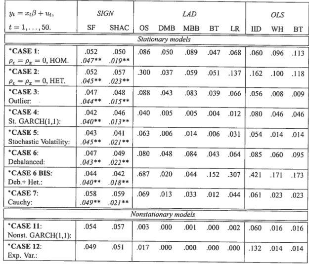
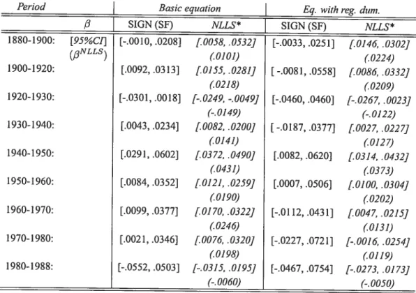
1 Confidence intervals 31
2 Simulated models 37
3 Linear regression under mediangale errors: empirical sizes of conditional
tests for H0: (1,2,3)’ 40
4 Linear regression with serial dependence: empirical sizes of conditional tests forH0 : /3z (1,2,3)’
41
5 Width of confidence intervals 46
6 S&P price index: 95 % confidence intervals 49
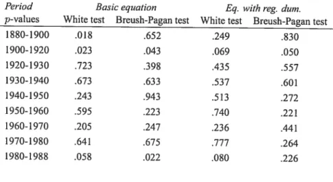
7 Regressions for personal income across U.S. States, 1880-1988 52 8 Regressions for personal income across U.S. States, 1820-198$: summary
ofregression diagnostics 64
9 Regressions for personal income across U.S. States, 1880-198$: tests for
heteroskedasticity 64
10 Regressions for personal income across U.S. States, 1880-1988: prelimi
nary resuits 75
11 Regressions for personal income across U.S. States, 1880-1988: comple
mentary resuits 76
12 Simulated models 109
13 Sirnulated bias and RMSE 111
14 Constant and drift estimates 113
15 Regressions for personal income across US. $tates, 1880-1988 117
16 Summary ofregression diagnostics . . 128
17 Empirical sizes: n50 165
18 Confidence intervals for schooling returns 174
19 Estimates for schooling retums 174
20 Confidence intervals for schooling returns: subsamples n=1 0000 and n2000 175 21 Estirnates for schooling retums: subsamples ‘n=10000 and n=2000 . . . . 175
xi
Table des figures
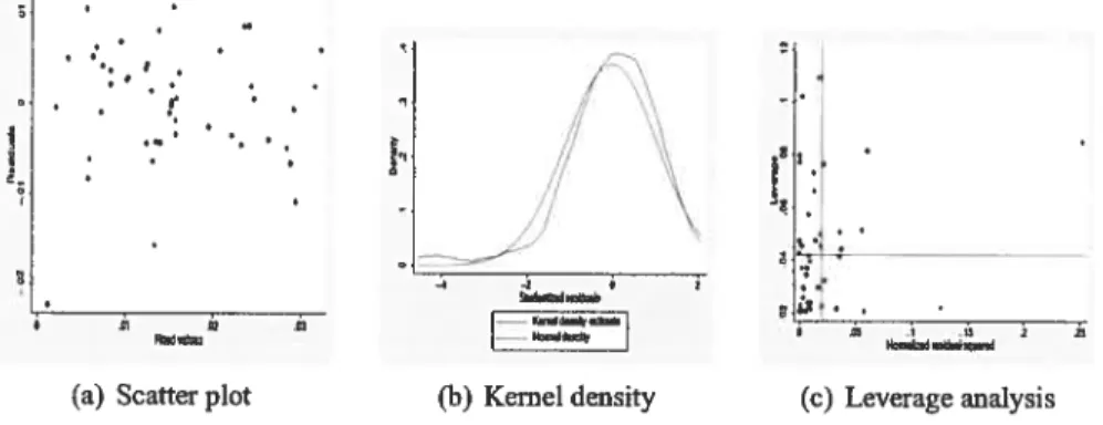
2 Power functions (level corrected) (1) 3 Power functions (level corrected) (2)
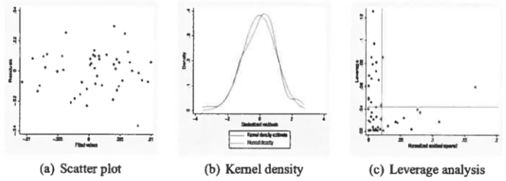
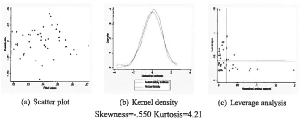
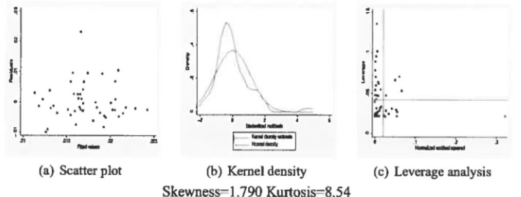
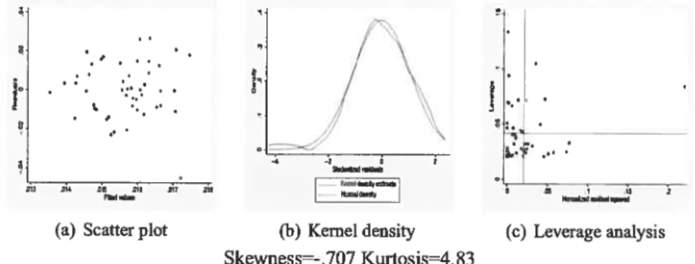
5 Residual analysis: basic equation 6 Residual analysis: basic equation 7 Residual analysis: basic equation 8 Residual analysis: basic equation 9 Residual analysis: basic equation 10 Residual analysis: basic equation 11 Residual analysis: basic equation 12 Residual analysis: basic equation 13 Residual analysis: regional dummies 14 Residual analysis: regional dummies 15 Residual analysis: regional dummies 16 Residual analysis: regional dummies 17 Residual analysis: regional dummies 18 Residual analysis: regional dummies 19 Residual analysis: regional dummies 20 Residual analysis: regional dummies 21 Residual analysis: regional dummies
30 1880-1900 70 92 93 94 95 96 129
1 Confidence regions provided by Sf-based inference
4 Residual analysis: basic equation 1880-1900 1900-1920 1920-1930 1930-1940 1940-1950 1950-1960 1960-1970 1970-1980 1980-198$ 1900-1920 1920-1930 1930-1940 1940-1950 1950-1960 1960-1970 1970-1980 980-1988
22 Sirnulated confidence distribution cumulative function based on SST . 23 Simulated p-value functions based on SST and SF
24 Simulated p-value functions based on SST and SF when the parameter is badly identified
25 Simulated p-value functions 26 Projection-based p-values
28 Concentrated statistics and projected p-values (1930-1960) 130 29 Concentrated statistics and projected p-values (1960-1988) 131
30 Power functions: model with one instrument 168
3 1 Power functions: model with five instruments 169
32 Power functions: model with one instrument: heteroskedastic cases . 170
Remerciements
Je tiens tout d’abord à remercier tous ceux que je risque d’oublier par la suite. A coup de petits riens, nombreux sont ceux qui ont contribué à ce travail.
Je remercie mes directeurs. D’abord pour avoir bien voulu tenter l’expérience de la coti.ttelle. Et surtout, pour m’avoir guidée dans le monde de l’économétrie. Je tiens à expri mer toute ma gratitude à Jean-Marie Dufour. Son soutien et sa générosité m’ont accompa gné tout au long de cette thèse. C’est un honneur pour moi d’avoir pu travailler aux côtés de quelqu’un d’aussi brillant. Merci à Thierry Magnac pour ses conseils, son aide et sa confiance. Je regreffe que les circonstances ne nous aient pas amenés à collaborer plus di rectement. Je retiendrai de leurs enseignements, entre autres, qu’un bon chercheur doit être armé d’une bonne dose de patience mais qu’il doit aussi être capable de se lancer.
Je remercie Marc Hallin et Frédéric Jouneau d’avoir accepté d’être examinateur ex terne et rapporteur de cette thèse. Je remercie Marine Carrasco, Silvia Gonçalves et Alain Trognon d’avoir accepté de composer mon jury, même au prix d’un voyage à Montréal.
Je remercie les laboratoires et institutions qui m’ont accueillie et financée le CRDE CIREQ et le département de sciences économiques de l’université de Montréal, puis, le laboratoire de microéconométrie appliquée du CREST et l’INSEE qui m’a aidée à conti nuer ma recherche après ma réussite au concours et soutenue dans ce projet. Je pense aux autres administrateurs de l’INSEE qui ont aussi entrepris une thèse. Je les encourage dans cette démarche comme ils l’ont fait pour moi.
Je remercie les participants aux séminaires et aux conférences auquels j’ai pris part pour leurs remarques constructives. Merci à Nour Meddahi pour ses conseils sur le deuxième chapitre; à Hélène et Jan Johannes qui, en plein mois d’août, ont plongé dans une version préliminaire du troisième et à Charlotte Hardouin, pour ses conseils téléphoniques mathé matiques. Merci à Pascale Valéry qui m’a fourni les données de l’application sur l’indice s&P.
Je remercie Pascal Martinolli et ses prouesses bibliothèquesques. Sans lui, elle (en) serait loin cette thèse!
et étudiants, avec lesquels j’ai sympathisé (la liste est longue...). Et, parmi eux tous mes co-bureaux! Merci pour nos discussions, votre ambiance et vos sourires!
Je remercie Lucie, Lyne et Luc qui m’ont apporté un vrai chez-nous (acado-)québécois, c’est-à-dire rempli de chaleur.
Enfin, je remercie Etienne et ses multiples facettes qui vont de ta hot-tine informatique à l’intendance domestique, en passant par une intarissable source de «niaque».
Intro
ducfion
Tout le monde croit aux erreurs normales, disait Henri Poincaré1, les mathématiciens parce qu’ils s’imaginent que c’est un fait d’observation, et les observateurs que c’est un théorème mathématique.
Quand en économétrie, on relâche l’hypothèse de normalité des erreurs, c’est très souvent pour y revenir en ayant recours à des approximations asymptotiques. Ainsi, l’inférence « à la Wald » est couramment utilisée : on calcule un estimateur, puis son comportement asymptotique grâce à un théorème central limite, on en déduit ensuite des tests et des ré gions de confiance asymptotiques.
Pourtant, de nombreuses études empiriques ou par simulation soulignent les limites des approximations asymptotiques. Les exemples de tests qui présentent des distortions de niveau en échantillon fini sont nombreux [pour des exemples eti séries temporelles, voir Dufour (1981), Campbell et Dufour (1995, 1997) et dans le contexte d’une régression sur la médiane, voir Buchinsky (1995), DeAngelis, Hall et Young (1993), Dielman et Pfaffen berger (19$8a, 1988b)]. La normalité qu’elle soit imposée par le modèle paramétrique ou approchée en asymptotique ne vient donc pas toujours d’un fait d’observation.
Les limites des méthodes asymptotiques sont aussi bien connues dans la littérature sta tistique. On sait depuis Bahadur et Savage (1956) qu’il n’existe pas de procédure de test valide et puissante en échantillon fini pour tester une moyenne si on ne spécifie pas plus ta forme de la distribution. La conséquence en est qu’à distance finie, un test basé sur la distribution asymptotique a une taille qui peut arbitrairement dévier de son niveau nominal. En d’autres termes, la moyenne n’est pas testable dans un modèle non paramétrique. Pour décrire une procédure de test qui soit valide en présence d’hétéroscédasticité de forme ar bitraire, il est nécessaire de recourir â une mesure de localisation, comme la médiane. Lehmann et Stem (1949) nous indiquent par ailleurs qu’il existe des procédures robustes à l’hétéroscédasticité de forme arbitraire : les procédures basées sur les signes. Ces deux résultats de la théorie des tests impliquent, entre autres, que les méthodes asymptotiques,
Plus précisément, Henri Poincaré rapporte les dires d’un collègue dans la préface de son ouvrageTher
modenarnique, 1908 «un physicien éminent me disait un jour à propos de la loi deserreurs tout le monde y croit fermement parce que les mathématiciens s’imaginent que c’est un fait d’observation, et les observateurs que c’est un théorème mathématique.»
en particulier celles qui s’appuient sur la moyenne, ne permettent pas de contrôler le ni veau des tests en échantillon fini, et ce, même lorsque qu’elles sont dites « corrigées de
l’hétéroscédasticité et de l’autocorrélation (HAC) ». Elles ne sont pas valides à distance finie. Utiliser la normalité asymptotique n’est donc pas toujours ce que conseillerait un théoricien.
Un autre épisode de l’histoire économétrique a renforcé la méfiance que peut inspi rer l’inférence « à la Wald» : celui des instruments faibles. Lorsqu’un modèle structurel fait intervenir des variables explicatives endogènes, c’est-à-dire corrélées avec le terme d’erreur, ona habituellement recours à des méthodes instrumentales. Les instruments sont
des variables auxiliaires exogènes, c’est-à-dire non corrélées avec le terme d’erreur, qui vont assurer l’identification des paramètres du modèle et permettre d’inférer sur leurs va leurs. Pour ce faire, ils doivent être pertinents, c’est-à-dire bien corrélés avec les variables explicatives endogènes. Lorsqu’ils ne le sont que Jaiblement, ils ne permettent pas de re trouver une bonne identification du paramètre (cas de non-identification ou de quasi-non identification). En présence d’instruments faibles ou en l’absence d’identification, les sta tistiques de type Wald ont des comportements asymptotiques inhabituels et les tests asymp totiques qui en découlent ne sont pas valides.
La littérature sur les instruments faibles met fortement en garde contre les défauts des méthodes asymptotiques habituelles qui s’appuient sur une hypothèse d’identification et sur la normalité asymptotique des estimateurs. Elle rappelle aussi qu’if existe des statistiques pivotales robustes aux problèmes d’identification à partir desquelles on peut construire des tests valides. La première d’entre elles est la statistique d’Anderson et Rubin (AR) [Anderson et Rubin (1949)]. D’autres ont suivi [Kleibergen (2002, 2005, forthco ming), Moreira (2001, 2003), voir aussi Dufour et Jasiak (2001), Stock et Wright (2000), Dufour et Taamouti (2005), ..
.].
Cette littérature amène à réfléchir sur la mise en oeuvre de l’inférence. Elle remet l’accent sur l’importance des statistiques pivotales.Partir des tests et d’une statistique pivotale pour en dériver un système d’inférence est classique en statistique. Cette démarche permet de plus de redécouvrir différentes notions moins communément utilisées en économétrie.
Encore faut-il que de tels pivots soient disponibles. C’est à cela que répond le résultat de Lehmann et Stem en échantillon fini, dans un modèle avec hétéroscédasticité de forme arbitraire, une transformation par les signes peut aider à construire des pivots.
Dans cette thèse, nous proposons un système d’inférence exacte en échantillon fini pour des modèles de régression semi-paramétriques sur la médiane. A partir de statistiques pivo tales basées sur les signes des résidus, nous construisons des tests de Monte Carlo [Dwass (1957), Bamard (1963), Dufour (2006)] qui exploitent la distribution exacte de ces statis tiques. Le niveau de ces tests simultanés est contrôlé quelle que soit la taille de l’échantillon et ce, pour des formes arbitraires d’hétéroscédasticité et de dépendance non-linéaire. Nous construisons ensuite des régions de confiance simultanées en inversant ces tests, et des tests d’hypothèses plus générales grâce à des techniques de projection [Dufour et Kiviet (1998), Dufour et Jasiak (2001), Dufour et Taamouti (2005)]. Nous étudions ensuite d’autres outils d’inférence qui ont jusqu’à présent reçu moins d’écho dans la littérature économétrique la fonction p-value et la distribution de confiance. L’estimateur constitue enfin la dernière brique de ce système d’inférence. Cette approche inférentielle commence donc par les tests et finit par l’estimateur puisque celui-ci ne présente d’intérêt que si te paramètre est identi fiable.
Différents modèles sont étudiés tout au long de la thèse. Nous commençons par un modèle de régression linéaire, puis nous étendons la méthode aux régressions non-linéaires et aux modèles structurels. Cette thèse se compose de trois essais.
Nous étudions dans le premier essai la construction de tests et de régions de confiance dans un modèle de régression linéaire sur la médiane. Nous supposons que le processus d’erreur est de médiane nulle conditionnellement aux variables explicatives et à son propre passé sans imposer de restriction paramétrique supplémentaire sur sa distribution. Celle-ci peut être nongaussienne, hétéroscédastique ou bien présenter une dépendance sérielle de
forme arbitraire, ce qui inclut les processus ARCH, GARCH et de volatilité stochastique. Seule est exclue dans un premier temps la dépendance linéaire. La transformation par les signes des résidus contraints permet de définir des statistiques de test dont la distribution
ne dépend pas de paramètres de nuisance et est aisément simulable quelle que soit la taille de l’échantillon. La méthode des tests de Monte Carlo ainsi que celle des projections nous permettent tour à tour de construire des tests simultanés exacts et des régions de confiance pour le vecteur de paramètres, puis des tests et des régions de confiance valides pour n’im porte quelle transformation possiblement non linéaire, et ce, quelle que soit la taille de l’échantillon.
En revanche, les statistiques de signes que nous utilisons ne sont plus pivotales lorsque le processus d’erreur est linéairement dépendant (cas d’un ARMA stationnaire, par exemple). La matrice de variance asymptotique constitue dans ce cas un paramètre de nuisance. Les méthodes HAC standard nous permettent de le corriger asymptotiquement. La procédure de Monte Carlo développée précédemment est alors asymptotiquement va lide sous des hypothèses d’existence de moment et de densité plus faibles que les méthodes asymptotiques habituelles. De plus, elle ne requiert pas d’approximer des paramètres in connus (ce qui, au contraire, constitue une des principales difficultés des méthodes des noyaux par exemple).
Les études par simulation suggèrent qu’elle est plus performante que les méthodes asymptotiques habituelles pour des processus très hétérogènes ou lorsque la taille de l’échantillon est petite. Cette méthode est donc particulièrement adaptée à l’étude des données financières qui sont souvent très hétéroscédastiques ainsi qu’aux analyses qui s’appuient sur un faible nombre d’observations (séries temporelles, études inter-régionales, données d’enquête, .
.
L’approche inférentielle basée sur les tests permet de mettre en avant d’autres outils moins communément utilisés en économétrie. Dans le deuxième essai, nous reprenons et étudions, la notion de distribution de confiance associée à une statistique de test qui est une réinterprétation des distributions fiducielles de Fisher [f isher (1930), Efron (199$), Schwe der etHjort (2002)]. La fonction p-value qui en découle associe un degré de confiance à
chaque valeur testée du paramètre, étant donnée la réalisation des données. Distributions de confiance et fonctions p-value constituent un équivalent fréquentiste aux distributions a posteriori bayésiennes. Elles résument les résultats des tests et en donnent une
illustra-tion graphique. La distribuillustra-tion de confiance est pourtant rarement utilisée en économétrie car elle ne se définit aisémment que dans le cas d’un paramètre réel et requiert l’utilisation d’une statistique pivotale. La fonction p-value peut, elle, être étendue au cas d’un paramètre multidimensionnel. Notre objectif est d’étendre ces notions au cas multidimensionnel dans le contexte d’une régression sur la médiane. La transformation par les signes nous permet de construire des statistiques pivotales sans recourir à des hypothèses paramétriques. Nous calculons des fonctions p-value simulées à partir de tests de Monte Carlo, puis des versions projetées pour chaque composante individuelle du paramètre. Celles-ci donnent à la fois une illustration graphique de l’inférence et du degré d’identification du paramètre. Cepen dant, comme elles s’appuient sur des statistiques discrètes, nous n’avons que des versions approchées des notions initiales.
Le deuxième objectif de cet essai est d’associer un estimateur à la procédure d’infé rence. Pour ce faire, nous suivons le principe d’inversion de test de Hodges et Lehmann [Hodges et Lehmann (1963)], et proposons d’utiliser comme estimateur la valeur du para mètre associé au plus haut degré de confiance (soit à la plus forte p-value). Nous montrons que l’estimateur de signe qui en découle est sans biais pour la médiane quand les erreurs sont symétriques et qu’il partage les propriétés d’équivariance de l’estimateur « Least Ab solute Deviations (LAD) ». Il est aussi convergent et asymptotiquement normal sous des conditions plus faibles que l’estimateur LAD.
En échantillon fini, tes simulations suggèrent qu’il est supérieur à t’estimateur LAD, du point de vue du biais et de l’erreur quadratique moyenne, pour des processus très hétéroscédastiques ou possédant des queues de distribution épaisses.
Le troisième essai porte sur les modèles structurels et non-linéaires. L’échec des mé thodes asymptotiques usuelles dans les modèles structurels motive fortement une étude à distance finie. Pourtant, la plupart des procédures disponibles dans la littérature s’appuient sur un modèle paramétrique ou ne sont qu’asymptotiquementjustifiées. Dans un cadre non paramétrique, seules les procédures de rang ont été adaptées aux échantillons finis. Ce troi sième essai présente une procédure valide quelle que soit la taille de l’échantillon et robuste à l’hétéroscédasticité de forme arbitraire. Nous utilisons une version de la propriété de
pi-votalité des signes adaptée à un modèle avec instruments. Les tests qui en découlent sont exacts et ne dépendent pas du degré d’identification du paramètre. Ils restent valides en présence d’instruments faibles ou de problème d’identification du paramètre.
L’approche que nous suivons peut aussi s’interpréter en termes de régressions artifi cielles. Les signes des résidus contraints sont régressés sur des instruments auxiliaires dans l’esprit d’Anderson et Rubin tAnderson et Rubin (1949), Dufour (2003)]. Ce type de pro cédure a cependant le défaut de perdre de la puissance lorsque beaucoup d’instruments sont utilisés. Ceci pose la question des instruments à inclure dans le modèle en cas de suri dentification. Nous étudions deux concepts d’optimalité et proposons d’utiliser la méthode de partage de l’échantillon
[
«spiit sample », Dufour et Jasiak (2001)] pour calculer des versions approchées de ces instruments optimaux.Les simulations montrent que notre approche est supérieure aux méthodes usuelles (y compris celles qui sont robustes à la présence d’instruments faibles) lorsque les erreurs sont non gaussiennes et hétéroscédastiques.
Chapitre 1
Finite-sample distribution-free inference in linear median
regressions under heteroskedasticity and nonhinear
1.
Introduction
The Laplace-Boscovich median regression has received a renewed interest since two decades. This method is known to be more robust than least squares and easily allows for heterogeneous data [see Dodge (1997)]. It has recently been adapted to models in volving heteroskedasticity and autocorrelation [Zhao (2001), Weiss (1990)], endogeneity [Amerniya (1982), Poweil (1983), Hong and Tamer (2003)], nonlinear functional forms [Weiss (1991)] and has been generalized to other quantile regressions [Koenker and Bas sett (197$)]. Theoretical advances on the behavior ofthe associated estimators have com pleted this process [Poweil (1994), Chen, Linton, and Van Keilegom (2003)]. In empincal studies, partly thanks to the generalization to quantile regressions, new fieÏds of potential applications were bom.’ The recent and fast development of computer technology clearly stimulates interest for these robust, but formerly viewed as too cumbersome, methods.
Linear median regression assumes a linear relation between the dependent variable y and the explanatoiy variables x. Only a nuli median assumption is imposed on the dis turbance process. Such a condition of identification “by the median” can be motivated by fundarnental resuits on nonparametric inference. Since Bahadur and Savage (1956), it is known that without strong distributional assumptions (such as normality), it is impossible to obtain reasonable tests on the mean ofi.i.d. observations, for any sample size. Moments are not empirically meaningful without any further distributional assumptions. This form
of non-identification can be etiminated, even in finite samples, by choosing another
mea-sure of central tendency, such as the median. Hypotheses on the median of non-normal observations can easily be tested by signs tests [see Pratt and Gibbons (1981)]. In nonpara metric setups, one may expect models with median identification to be more appropriate than their mean counterpart.
Median regression (and related quantile regressions) provides an attractive bridge be tween parametric and nonparametric models. Distributional assumptions on the distur bance process are relaxed but the functional form remains parametric. Associated estima
‘The reader is referred to Buchinsky (1994) for an interpretation intermsof inequality and mobility topics in the U.S. labor market, Engle and Manganelti (1999) for an application in Value at Risk issues in finance
tors, such as the least absolute deviations (LAD) estimator, are more robust to outiiers than usua! LS methods and may be more efficient whenever the median is a better measure of location than the mean. This holds for heavy-tailed distributions or distributions that have mass at zero. They are especiaily appropriate when unobserved heterogeneity is suspected in the data. The current expansion of such sernipararnetric” techniques refiects an inten tion to depart from restrictive parametric framework [see Poweil (1994)]. However, reiated inference and confidence intervals remain based on asymptotic normality approximations. This reversai to normal approximate inference is certainiy disappointing when so much effort bas been made to get rid ofparametric modeis.
In this paper, we show that a testing theory based on residual signs provides an entire system of finite-sample exact inference for a linear median regression mode!. The !eve! of the tests is provably equal to the nominal level, for any sample size. Exact tests and confidence regions rernain valid under general assumptions involving heteroskedasticity of unknown form and nonlinear dependence.
The starting point is a weli known resuit of quasi-irnpossibiiity in the non-parametric statisticai literature. Lehmann and Stem (1949) proved that inference procedures that are valid under conditions of heteroskedasticity ofunknown form when the number of observa tions is finite, must contro! the level ofthe tests conditiona! on the abso!ute values [see also Pratt and Gibbons (1981), Lehmann (1959)]. This result has two main consequences. First, sign-based methods, which do controi the conditionai ievei, are a generai way0f producing vaiid inference for any sampie size. Second, ail other methods, including the usuai het eroskedasticity and autocorrelation corrected (HAC) methods developed by White (1980), Newey and West (1987), Andrews (1991) and others, which are flot based on signs, are not proved to be vaiid for any sample size. Aithough this provides a compelling argument for using sign-based procedures, the latter have barely been exploited in econometrics. Our point is to stress their robustness and to generalize their use to median regressions.
To our knowiedge, sign-based methods have flot received much interest in economet rics, cornpared to ranks or signed ranks methods. Dufour (1981), Carnpbell and Dufour (1991, 1995), Wright (2000), derived exact nonparametric tests for different time series modeis. In a regression context, Boldin, Simonova, and Tyurin (1997) deveioped inference
and estimation for linear models. Thcy presented both exact and asymptotic-based infer ences for i.i.d. observations, whereas for autoregressive processes with i.i.d. disturbances, only asymptotic justification was available. Our work is positioned in the following of Boldin, Simonova, and Tyurin (1997). We keep sign-based statistics related to locally opti mal sign tests, which are simple quadratic forms and can easily be adapted for estimation. However, we extend their distribution-free properties to allow for a wide array of nonlinear dependent schemes. We propose to conjugate them with projection tecimiques and Monte Carlo tests to systernaticalty derive exact confidence sets.
The pivotality ofthe sign-based statistics validates the use of Monte Carlo tests, a tech nique proposed by Dwass (1957) and Bamard (1963). The Monte Carlo metliod, adapted to discrete statistics by a tie-breaking procedure [Dufour (2006)], yields exact simultaneous confidence region for 3. Then, conservative confidence intervals (CIs) for each component ofthe parameter (or any real function of the parameter) are obtained by projection [Dufour and Kiviet (1998), Dufour and Taamouti (2005), Dufour and Jasiak (2001)]. Exact Cis as they are valid can be unbounded for nonidentifiable component. That resuits from the ex actness of the method and insures the tme value of the component belongs to exact CIs with probability higher than 1 — c. In practice, computation of bounds of confidence intervals
(or confidence sets) requires global optimization algorithrns such as simulated annealing [see Goffe, ferrier, and Rogers (1994)].
Sign-based inference methods constitute an alternative to inference derived from the as ymptotic behavior of the well known LAD estimator. The LAD estimator (such as related quantile estimators) is consistent and asymptotically normal in case of heteroskedasticity [PowelI (1984) and Zhao (2001) for efficient weighted LAD estimator], or temporal de pendence [Weiss (1991)]. fitzenberger (1997b) extended the scherne ofpotential temporal dependence including stationary ARMA disturbance processes. Horowitz (1998) proposed a smoothed version of the LAD estimator. At the same time, an important problem in the LAD literature consists in providing good estimates of the asymptotic covariance matrix, on which inference relies. Poweil (1984) suggested kemel estimation, but the most wide spread method of estimation is the bootstrap. Buchinsky (1995) advocated the use of design matrix bootstrap for independent observations. In dependent cases, fitzenberger (l997b)
proposed a moving block bootstrap. Finally, HaIm (1997) suggested a Bayesian bootstrap.2 Other notable areas of investigation in the L1 literature concem the study of nonlinear ffinctional forms and structural models with endogeneity {“censored quantile regressions”, Poweil (1984, 1986) and Fitzenberger (l997a), Buchinsky and J. (1998), “simultaneous equations”, Amemiya (1982), Hong and lamer (2003)]. More recently, authors have been interested in allowing for misspecification [Kim and White (2002), Komunjer (2005), Jung (1996)].
In the context of LAD-based inference, kernel techniques are sensitive to the choice of kemel function and bandwidth parameter, and the estimation of the LAD asymptotic covariance matrix needs a reliable estimator ofthe error term density at zero. This may be tricky especially when disturbances are heteroskedastic. Besides, whenever the normal dis tribution is flot a good finite-sampie approximation, inference based on covariance matrix estimation may be problematic. from a finite-sampie point ofview, asymptoticaliyjustified methods can be arbitrariÏy unreliable. Test levels can be far from their nominal size. One can find examples of such distortions for time series context in Dufour (1981), Campbell and Dufour (1995, 1997) and for L1-estimation in Buchinsky (1995), De Angelis, Hall, and Young (1993), Dielman and Pfaifenberger (1988a, 1988b). Inference based on signs constitutes an alternative that does flot suifer from these shortcomings.
We study here a linear median regression model where the (possibly dependent) distur bance process is assumed to have a nuil median conditional on some exogenous explanatory variables and its own past. Ibis setup covers non stochastic heteroskedasticity, standard conditional heteroskedasticity (like ARCH, GARCH, stochastic volatility models,
...)
as well as other forms of nonlinear dependence. However, linear autocorrelation in the resid uals is not allowed. We first treat the problem of inference and show that pivotai statistics based on the signs of the residuals are available for any sample size. Hence, exact infer ence and exact simuttaneous confidence region on /3 can be derived using Monte Carlo tests. For more general processes that may involve stationary ARMA disturbances, these statistics are no longer pivotal. The serial dependence parameters constitute nuisance pa2The reader is referred to Buchinsky (1995, 1998), for a review and to Fitzenberger (1997b) for a com parison between these methods.
rameters. However, transforming sign-based statistics with standard HAC methods allows to asymptotically get rid of these nuisance pararneters. We thus extend the validity of the Monte Carlo method. For these kinds of processes, we loose the exactness but keep an asymptotic validity. In particular, this asymptotic validity requires less assumptions on moments or the shape of the distribution (sucli as the existence of a density) than usual asymptotic-based inference. Besides, we do flot need to evaluate the disturbance density at zero, which constitutes one of the major difficulties of kernel-based rnethods. In practice, we derive sign-based statistics from locally most powerful test statistics. We obtain exact simultaneous confidence region and then, conservative confidence intervals for each com ponent or any real function of 3 by projection techniques. Once again, we stress the fact that sign-based statistics can provide finite-sample inference which is flot the case for usual inference theories associated with LAD and other quantile estimators, which rely on their
asymptotic distributions.
The paper is organized as follows. In section 2, we present the model and the notations. Section 3 contains general resuits on exact inference. They are applied to median regres sions in section 4. In section 5, we derive confidence intervals at any given confidence level and illustrate the method on a numerical example. Section 6 is dedicated to the asymptotic validity of the finite-sample inference method. In section 7, we give simulation resuits from comparisons to usual techniques. Section 8 presents illustrative applications: testing the presence of a drift in the standard and poor’s composite price index series, and testing for 3 convergence between levels of per capita output across the U. S. States. Section 9 concludes. Appendix A contains the proofs.
2.
Framcwork
2.1.
Model
We consider a stochastic process W {W, (Yt, x) : Q — R»l, t = 1,2,
.
. .}
definedon a probability space (Q, F, P). Let {l47, FL} t=1,2,... be an adapted stochastic sequence,
o-(W1,.
..
,W) is the u-algebra spanned by W1,... ,W. W = (y, x), where y is thedependent variable and xt = (Xti,. .. ,x)’, a p-vector of explanatory variables. The xt‘S
may be random or fixed.
We assume thatYt andXt satisfy a linear model and we shall impose in the following some
conditions on the median ofthe disturbance process:
yj xt3+u, t 1,... ,n. (2.1)
In the following, y = (yi, .
-
y1)’e
R’ stands for the dependent vector, X = [xifor the n x p explanatoiy matrix. /3
e
R is the vector of parameters, andn = (n1,
. ..
,n,)’e
R’ the disturbance vector. Moreover, the distribution functionof’u conditional on X is denoted
Ft(.Ixi,.
.. ,xv).in the classical linear regression framework, {n, t = 1, 2,.
.
.}
is assumed to be amartingale difference with respect to J = cr(Wi,. .. , W,), t = 1, 2
Definition 2.1 MARTINGALE DIFFERENCE. Let {Ut,J : t = 1, 2, .
. .}
be an adaptedstochastic sequence. Then {u, t = 1, 2,
..
.}
is a martingale dfference sequence withrespect to {.T, t = 1, 2,
.} /ff
= O, Vt> 1.
We depart from this usual assumption. Indeed, our aim is to develop a framework that is robust to heteroskedasticity of unknown form. from Bahadur and Savage (1956), it is known that inference on the mean ofi.i.d. observations of a random variable without any further assumption on the form of its distribution is impossible. Such a test has no power. This problem of non-testability can be viewed as a form of non-identification in a wide sense. Unless relatively strong distributional assumptions are made, moments are not em pirically meaningftil. Thus, if one wants to relax the distributional assumptions, one must choose another measure of central tendency such as the median. The median is in particular weli adapted if the distribution of the disturbance process does flot possess moments. As
a consequence, in this median regression framework, the martingale difference assumption will be replaced by an analogue in terms ofrnedian. We define the median-martingale dif ference or shortly said, inediangaÏe that can be stated unconditional or conditional on the design matrix X.
Definition2.2 STRICT MEDIANGALE. Let t = 1,2...}beanadaptedsequence.
Then {rit, t = 1, 2,
.
. .}
is a strict mediangale with respect to {F, t = 1, 2,. . .} (if
P[ui <0] = P[ui > 0] = 0.5,
P[u <
0IF_i]
P{u >0IF_i]
0.5,fort > 1.Definition2.3 STRICT CONDITIONAL MEDIANGALE. Let t 1,2..
.}
bean adapted sequence and F = u(uY,.
.
,u,, X). Then {Ut, t = 1,2,..
.}
is a strictmediangale conditionalonX with respect to
{,
t = 1,2,.. .} ff
P[ui <OIX] = P[ui > OIX] = 0.5,
P[u <Ojui,...,’ut_i,X] = P[u > 0ju1,...,u_1,X] =0.5, fort >1.
Note that the above distributions allow rit to have a discrete distribution except at zero. 1f the latter constraint is retaxed, we get that following definition.
Definition 2.4 WEAK CONDITIONAL MEDIANGALE. Let {rit, t = 1, 2.
. .}
be anadapted sequence and 1 = u(u1,... ,rit,X). Then {Ut, t 1, 2,.
.}
is a weak median gale conditionalonX with respect to {F, t = 1,2,.. .1
‘ff
P{n1 > OjX] P[ui <0X],
The sign operators R —* {—1, O, 1} is defined as
f
1, ifa E A,s(a) = 1[o,+)(a) — 1(_,o](a), 1A(a) = (2.2)
L.
O, ifa A.For convenience, the notation wifl be extended to vectors. Let n e R” and s(n), the n
vector composed by the signs ofits components. Stating that {Ut, t = 1, 2,.
.
.}
is a weak mediangale with respect to {F, t 1, 2,.
. is exactly equivalent to assuming that{3(Ut), t = 1,2,
. . .}
is a martinga’e difference withrespect to the same sequence of sub-o- algebras {F, t = 1, 2,
.
.
.}.
However, the weak conditional mediangale concept as defined before differs from a martingale difference on the signs because of the conditioning upon X. Indeed, the reference sequence of sub-u algebras is usually taken to{
u(Wi,. . .
, W), t = 1, 2,.. .}.
Here, the referencesequence is {F = u(W1,. . ,W, X), t = 1,2,.
.
.}.
Conditional mediangale requires conditioning on the whole process X. We shah see later that asymptotic inference may be available under weaker assumptions, as a classical martingale difference on signs or more generally some mixing concepts on {S(Ut),u(W1,...
, t = 1,2,..
.}.
However, the conditional mediangale concept allows one to develop exact inference (conditional on X).We have replaced the difference of martingale assumption on the raw process {Ut, t =
1,2,.
.
.}
by a quasi-simihar hypothesis on a robust transform ofthis process {S(Ut), t 1, 2,. . .}.
Below we will see it is relatively easy to deal with a weak mediangale by a simple transformation of the sign operator. b simplify the presentation, we shah focus on the strict mediangale concept. Therefore, our model will rely on the fohlowing assumption. Assumption Al STRICT CONDITIONAL MEDIANGALE. The colnponents of u =(u1,. . . ,n,,) satisfy a strict rnediangaÏe conditional on X. It is easy to see that Assumption Al entails:
med(niIxi,...,x,,) =0,
Hence, we are in a median regression context. Our last remark concems exogeneity. As long as the Xt‘s are strongly exogenous explanatory variables,3 the conditional me diangale concept is equivalent to usual martingale difference for signs with respect to
J=o-(I’Vi,...,Wt), t=1,2
Proposition2.5 MEDIANGALEEXOGENEITY. Suppose {xt: t = 1,... ,n}isastrongly
exogenous processJôr t and
P{’ui > 0] P[’ui <0] = 0.5,
>
0j,
. . .
,u_y,xl,...
,x] = P[u <Oui,... ,ut_i,Xi,.. .
,x] = 0.5.Then {Ut, t N} is a strict mediangale conditional on X.
Model (2.1) with the Assumption AI allows forverygeneral forms ofthe disturbance dis
tribution, including asymrnetnc, heteroskedastic or dependent ones, as long as conditional medians are 0. We stress that neither density nor moment existence are required, which is an important difference with asymptotic theory. Indeed, what the mediangale concept requires is a form of independence in the signs of the residuals. This extends resuits in
Dufour (1981) and Campbell and Dufour (1991, 1995, 1997).
Asymptotic normality of the LAD estimator is presented in its most general way in Fitzenberger(1997b). It holds under some mixing concepts on {S(Ut),u(Wi,
.
.. ,W), t =1, 2,
. .
.1
and an orthogonality condition between {S(ut), t = 1, 2,.. .}
and {Xt, t =1, 2,.
.
.}.
However, this requires additional assumptions on moments.4 With such a choice, testing is necessarily based on approximations (asymptotic or bootstrap). Here, we focusonvalid finite-sampi e inference without any further assumptiononthe form of the distrib
utions. In order to conduct a ffilly exact method, we have to consider Assumption Al. 3Xis strongly exogenous for if X is sequentially exogenous and ifY doesflot Granger causeX, [sec
Gouriéroux and Monfort (1995a)]
41n fitzenberger (1997b), LAD and quantile estimators areshown to be consistent and asymptoticalty normal ifamongst other, E[xtso(ut)j = O, Vt 1,...,n, densities exist and second-order moments for (Ut, Xt) arefinite.
2.2.
Special cases
The above ftamework obviously covers independence but also a large spectrum of het eroskedasticity and dependence pattems. For example, suppose that
= .. . ,x) , t = 1, . ..
whereE,. . . ,a, are i.i.d. conditional on X = [x1,. . . ,x,]’. More generally, many depen
dence schemes are also covered: for example, any model of the form zLy=
Ut = JttXi, ,Xti ,‘U1, , , t = 2, . . . , ri
where cy, ... , are independent with median O, u1(x1 Xt_i) and
Jt(Xi,. . . ,x,, ,n1, ... , ni), t = 2,. .. ,n are non-zero with probability one. In
time series context, this includes:
1. ARCH(q) with non-Gaussian noiseet:
• . u; ut—i)
= o + i_i + • • +ŒqU_q
2. GARCH(p, q) with non-Gaussian noiseset:
Xt_1 ,Ul, . . . , Ut_i)2 = û+iU_;+ +qU_q+7iU_i+
3. stochastic volatility models with non-Gaussian noiseset:
Ut exp(w/2)ret
G1Wt_1 + + aiW_+
The first example is especiatly relevant for cross-sectional data when procedures are ex pected to be robust to heteroskedasticity. Other examples present robustness properties to endogenous disturbance variance (or volatility) specification. Note again that the distur bance process does flot have to be second-order stationary. For nonstationary processes that satisfy the mediangale assumption, sign-based inference will work whereas ail infer ence procedures based on asymptotic behavior of estimators may fail or require difficuit validity proofs. Note finatly that the previous property is more general and does not specify explicitly the functional form ofthe variance in contrast with an ARCH specification.
3.
Exact finite-sample sign-based inference
The most common procedure for developing inference on a statistical model can be de scribed as follows. f irst, one finds a (hopefully consistent) estimator; second, the asyrnp totic distribution of the latter is established, from which confidence sets and tests are de rived. Here, we shah proceed in the reverse order. We study first the test problem, then build confidence sets, and finally estimators.5 Hence, resuits on the valïd finite-sample test problem will be adapted to obtain valid confidence intervals and estimators.
3.1.
Motivation
In econometrics, tests are often based on t or
x2
statistics, which are derived from asymptotically normal statistics with a consistent estirnator of the asymptotic covariance matrix. Unfortcinately, in finite samples, these first-order approximations can be very misleading. Test levels can be quite far from their nominal size: both the probability that an asymptotic test rejects a correct nuli hypothesis and the probability that a component oft3 is contained in an asymptotic confidence intervalmay differ considerably from assigned
nominal tevels. One can find examples of such distortions in the dynamic hiterature [see for example Dufour (1981), Campbell and Dufour (1995, 1997) and Mankiw and Shapiro (1986)]; on inference based on L1 estimators, see also Buchinsky (1995), De Angelis, Hall, and Young (1993), Dielman and Pfaffenberger (1988a, 1988b). This remark usually
motivates the use of bootstrap procedures. In a sense, bootstrapping (once bias corrected) is a way to make approximation doser by introducing artificial observations. However, the bootstrap stili relies on approximations and in general there is no guarantee that the level condition is satisfied in finite samples.
Another way to appreciate the nonvalidity of asymptotic methods in finite samples is to recali a theorem established by Lehmann and Stem (1949). Consider testing whether n observations are independent with common zero median:
H0 : X1, ... , X,, are independent observations
each one with a distribution symmetric about zero.
TestingH0 tums to check whether the joint distribution F,, of the observations belongs to the set ?- = {F,,
e
F,, : F,, satisfies H0} without any other restriction. In other words, H0 allows for heteroskedasticity ofunknown form. For this setup, Lehmann and Stem (1949) established the following theorem (recalled and proved in Pratt and Gibbons (1981), seealso Lehmann (1959).
Theorem 3.1 If a test has ÏeveÏ cifor H0, where O < ci < 1, then it must satisfy the condition
P{RejectingHo XH ...
IX]
ci zinderH0 . (3.2)The level of a valid test must equal ci conditional on the observation absolute values.
Theorem 3.1 also implies that any procedure that does flot satisfy condition (3.2) has size one. Note that procedures typically designated as “robust to heteroskedasticity” or “I-TAC” [see White (1980), Newey and West (1987), Andrews (1991), etc.] are flot proved to satisfy condition (3.2), so they can have size one for any sample size.
Sign-based procedures do satisfy this condition. Besides, as we will show in the next section, distribution-free sign-based statistics are available even in finite samples. They have been used in the statistical literature to derive nonparametric sign tests. The combina tion ofboth remarks give the theoretical basis for developing an exact inference method.
3.2.
Distribution-free pïvotal functions and nonparametric tests
When the disturbance process is a conditional mediangale, the joint distribution of the signs of the disturbances is completely determined. These signs are mutually independent equalling 1 with probability 1/2 and —1 with probability 1/2. We state more precisely this resuit in the following proposition. We see also that the case with a mass at zero can be covered provided a transformation in the sign operator definition.
Proposition 3.2 SIGN DISTRIBUTION. Under model (2.1), suppose the ermrs (u1,. . . , u) satisfy a strict mediangale conditional on X [x1,.. . ,x,]’. Then the vari
abless(u1),..., s(u) are i.i.d. conditional on X according to the distribution
P[s(ut) 1 xi, . .. ,x,] = P[s(u) = —lxi,... ,x,] = , t 1, . . . , n. (3.3)
More generally, this resuit holds for any combination of t = 1, .. ,n. 1f there is a
permutationii : i
—
j
such that mediangale property holds forj,
the signs are i.i.d..from the above proposition, it follows that the residual sign vector of the model con
strained to 43
s(y - Xt3) [s(yi -
x/3),
... , s(y - x/3)]’ (3.4)has a nuisance-parameter-free distribution (conditional on X), i.e. it is apivotai function.
its distribution is easy to simulate from a combination of n independent uniform Bernoulli variables. furthermore, any fiinction of the fonu
T = T(s(y —X/3), X) (3.5)
is pivotai conditionai on X. Once the form of T is specified, the distribution ofthe statistic
Using Proposition 3.2, it is possible to construct tests for which the size is fully and exactly controlled. Consider testing
H0(t30) t /3 =
/3
against H1(/30) t/3
/30.Under H0(/30), s(y — s(u), t = 1,... ,n. Thus, conditional on X,
T(s(y— /30X), X) T(S7,, X) (3.6)
where S, (Si s7) andi,••• ,s7, are i.i.d. random variables according to a uniform
Bernoulli distribution on {—1, 1}. A test with level c rejects the nuil hypothesis when
T(s(y—/30X), X) > CT(X,c) (3.7)
where cT(X, c) is the (1 —c)-quanti1e ofthe distribution of T(S7,, X).
This method can be extended to error distributions with a mass at zero, i.e.,
P[ui
>OIX]
= P[ui <0IX],
P[u > DIX, ‘u1, ... u_] = P[ut <DIX, ‘uy,..., u_jj, t 2. (3.8)
Besides dependence, this specification attows for discrete distributions with a probability mass at zero, i.e. we can have:
= O
IX,
‘uy, ... , u_] = p(X, u, ... , ‘u) > 0 (3.9)where the pt() are unknown and may vary between observations. A way out consists in modifjing the sign function s(x) as follows:
If’ is independent oft then, in-espective ofthe distribution oft,
P[(u,
)
= +1] = P[(u, V) = —Ï] = . (3.11)Proposition 3.3 RANDOM1ZED SIGN DISTRIBUTION. Suppose (2.1) holds with the as
sumption that u1, ... , u. belong to a weak mediangale conditional on X. Let V1, ... , V,
be i.i.d random variables following a U(O, 1) distribution independent of u and X. Then the variablest
4)
are j. j. U. conditional on X with the distributionP[t1X]=P[t=—ÏIX] =, t=1,...,n. (3.12)
Ail the procedures described above can be applied without any further modification.
4.
Regression sign-based tests
In this section, we present sign-based test statisties that are pivots and provide power against alternatives of interest. This will enabie us to build Monte Carlo tests relying on the exact distribution of those sign-based statistics. Therefore, the level of those tests is exactly controlled for any sample size.
4.1.
Regression sign-based statïstics
The ciass of pivotai functions studied in the previous section is quite general. So, we
wish to choose a test statistic (the form of the T function) that can provide power against alternatives of interest. Unfortunately, there is no uniformly most powerful test of
against 3 4/3e. Hence, different alternatives may be considered. for testing Ho(t30) :
=
against H1 (j3)
/3
i30 in model (2.1), we consider test statistics of the following form:Ds(30, !2) = s(y —X/30)’Xf2(s(y —X/30),X)X’s(y —X/30) (4.13)
where !2(s(y —Xt30), X) is ap x p weight matrix that depends on the constrained signs
s(y — X/30) under H0(/30). Moreover, Q(s(y
definite.
Statistics ofthe form D8(f30, Q) include as special cases the ones studied by Boldin, Simonova, and Tyunn (1997) and Koenker and Bassett (1982). Namely, on taking Q = I,
and !2 (X’X)’, we get:
$3(/3) = s(y — X430)’XX’s(y— X/30) =
IIX’s(y
—X/30)
112
(4.14)and
$F(/30) = s(y -X/30)’P(X)s(y -X/30) =
IIX’s(y
-
Xt30)II,1
(4.15)where P(X) X(X’X)’X’. In Boldin, Simonova, and Tyurin (1997), it is shown that
SB(/3) and SF(/30) can be associated with locally most powerful tests in the case of
i.i.d. disturbances under some regularity conditions on the distribution function (especially
[(O) = O).6 Their proof can easily be extended to disturbances that satisfy the mediangale
property and for which the conditional density atzero is the sarne ft(OIX) = f(OIX), Vt =
SF(f31) can be interpreted as a sign analogue of the Fisher statistic. More precisely, $F(f30) is a monotonic transformation of the Fisher statistic for testing y = O in the re
gressionofs(y —Xf30) on X:
s(y—X/30) =X’y+v. (4.16)
Wald, Lagrange multiplier (LM) and likelihood ratio (LR) asymptotic tests for M estimators, such as the LAD estimator, in L1 regression are developed by Koenker and Bassett (1982). They assume i.i.d. errors and a fixed design matrix. In that setup, the LM statistic for testing Ho(/30) /3 = f3tums out to be exactly the SF(/30) statistic. The same
6The power fiinction ofthe Iocally most powerful sign-based test knows the faster increase when departing from/. In the multiparameter case, the scalar measure required to evaluate that speed is the curvamre of the power function. Restricting on unbiased tests, Boldin, Simonova, and Tyurin (1997) introduced different localty most powerful tests corresponding to different definitions ofcurvature. SB(/30) maximizes the mean curvature, which is proportional to the trace ofthe shape [see Dubrovin, fomenko, and Novikov (Ch. 2, pp. 76-$6, 1984),or Gray (Ch. 21, pp. 373-380, 1998),fora presentation ofvarious curvature notions].
authors also remarked that this type of statistic is asymptoticalÏy nuisance-parameter-free. It does flot require one to estimate the density ofthe disturbance at zero contrary to LR and Wald-type statistics.
The Boldin, Simonova, and Tyurin (1997) interpretation can be extended to het eroskedastic disturbances. in such a case, the locally optimal test statistic associated with the mean curvature—i.e., the test with the highest power function in the vicinity ofthe nuli
hypothesis according to a trace argument—will be ofthe following form.
Proposition 4.1 In moUd (2.1), suppose the mediangale Assumption Al holds, and the disturbances are heteroskedastic with conditionat densities
f (.
IX),
i 1, 2 that are continuousÏy dfferentiabÏe around zero andsuch that f(OIX) = O. Then, tue Ïocallyoptimal sign test statistic associated with the mean curvature is
SB([3) s(y— X/30)’XX’s(y — X/30) (4.17)
where
f1(OX) O
f(OjX) X.
o
...
f(OIX)When the fj(OIx)’s are unknown, the optimal statistic is flot feasible. The optimal weights must be replaced by approximations, such as weights derived from the normal distribution. These test statistics can also be interpreted as GMM statistics which exploit the property that {St 0 x’, Y} is a martingale difference sequence. We saw in the first section that this property is induced by the mediangale Assumption Al. However, these are quite unusual GMM statistics. Indeed, the parameter of interest is not defined by moment conditions in explicit form. It is implicitly defined as the solution of some robust estimating equations (involving constrained signs):