HAL Id: hal-01697496
https://hal.archives-ouvertes.fr/hal-01697496
Submitted on 1 Feb 2018
HAL is a multi-disciplinary open access
archive for the deposit and dissemination of
sci-entific research documents, whether they are
pub-lished or not. The documents may come from
teaching and research institutions in France or
L’archive ouverte pluridisciplinaire HAL, est
destinée au dépôt et à la diffusion de documents
scientifiques de niveau recherche, publiés ou non,
émanant des établissements d’enseignement et de
recherche français ou étrangers, des laboratoires
Analysis Of Percussive Sounds
Mathieu Lagrange, Bertrand Scherrer
To cite this version:
Mathieu Lagrange, Bertrand Scherrer. Two-Step Modal Identification For Increased Resolution
Anal-ysis Of Percussive Sounds. DAFX, 2008, Espoo, Finland. �hal-01697496�
TWO-STEP MODAL IDENTIFICATION FOR INCREASED RESOLUTION ANALYSIS OF
PERCUSSIVE SOUNDS
Mathieu Lagrange, Bertrand Scherrer
Music Technology Area,
CIRMMT, McGill University,
Montreal, QC, Canada
[email protected]
ABSTRACT
Modal synthesis is a practical and efficient way to model sound-ing structures with strong resonances. In order to create realistic sounds, one has to be able to extract the parameters of this model from recorded sounds produced by the physical system of interest. Many methods are available to achieve this goal, and most of them require a careful parametrization and a post-selection of the modes to guarantee a good quality/complexity trade-off.
This paper introduces a two step analysis method aiming at an automatic and reliable identification of the modes. The first step is performed at a global level with few assumptions about the spectro/temporal content of the considered signal. From the knowledge gained with this global analysis, one can focus on spe-cific frequency regions and perform a local analysis with strong assumptions. The gains of such a two step approach are a better estimation of the number of modal components as well as a better estimate of their parameters.
1. INTRODUCTION
The analysis of percussive sounds is of interest for a broad range of applications, from musical instruments modeling [1] to the au-dio rendering of interactions between physical objects in virtual environments [2]. The modal approach is commonly considered due to its physical motivations, generality and efficiency.
Several approaches are available for estimating the parameters of the models from recorded sounds. Such analysis methods are numerous, and most of them can be casted in two different classes: the ones based on the classical Discrete Fourier Transform (DFT) and the parametric approaches [3] rooted in linear prediction mod-els.
Most state-of-the-art modeling methods [1, 2] consider a me-thod based on the DFT and most of the time require a manual selection of the components of interest. Despite their interesting theoretical motivations, parametric methods have until recently suffered from instability while considering realistic signals, i.e. recorded sounds. Badeau proposed in [4, 5] several improvements of a High-Resolution parametric method which enable us to con-sider this method for the analysis of recorded sounds. Again, a careful selection of the components of interest is needed in order to obtain a relevant model of the sound.
In this paper, we propose a two-step analysis method whose block-diagram is shown on Figure 1. The first step is a global analysis which provides insight about the spectro/temporal struc-ture of the analyzed sound. A second step allows us to identify relevant components by better modeling the energy within the fre-quency region of the modal tracks identified during the first step.
This second step is implemented using two different approaches: one based on Auto Regressive Moving Average (ARMA) analysis and the other on High-Resolution (HR) analysis.
The paper is structured as follows: the underlying sound model and some motivations are presented in Section 2. The first analysis step is then presented in Section 3, as well as the details about the two different implementations considered, based on the DFT and a High Resolution approach respectively. From the results of this analysis step, some high level knowledge is obtained by identify-ing and trackidentify-ing some modes as explained in Section 4. In turn, from this high level knowledge, we select some frequency regions likely to contain some modes of interest. As explained in Section 5 a focused analysis is performed over those regions to better es-timate their modal content. In particular, the number of modes is much better estimated. This step is implemented using two differ-ent methods, one relying on an Auto Regressive approach and the other on High Resolution techniques. Section 6 demonstrates the gain of using this two-step analysis scheme by performing an eval-uation over a set of synthetic modal data, and finally show-cases the approach on real data.
2. SOUND MODEL
In modal analysis of percussive sounds, the sounding structure is described in terms of its natural modes. These modes are them-selves characterized by their frequencies and quality factor. These parameters are closely related to the geometrical shape of the ob-ject under study, its physical properties (e.g. stiffness, Young mod-ulus) and on the boundary conditions (e.g. hinged or clamped ends for example) [6]. The amplitude and phase of each mode strongly depends on the excitation provided to the physical structure.
Thus in order to extract all parameters necessary for modal analysis, we can use a model of the form of:
x(t) =
K
X
k=1
Akeδktej(2πfkt+φk)+ w(t) (1)
where x(t) is a sample of the observation at time t ∈ Z, K is the number of exponentially damped cisoids (a.k.a. the order of the model), (Ak, φk, fk, δk) are the amplitude, phase, frequency and
damping factor of the kthcomponent. The model also includes a white noise w(t) to account for the part of the sound that does not exactly fit the model. In order to model a real signal x(t) ∈ R, with Ns sinusoids, we need a model of order K = 2.Ns with
Figure 1: Block diagram of the proposed analysis methods.
3. BROAD-BAND ANALYSIS STEP
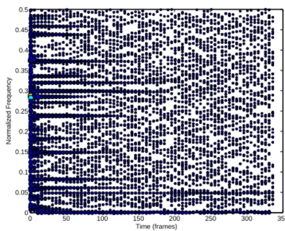
With this first analysis step, one would like to gain insight about the time/frequency distribution of the energy of the analyzed sig-nal. To achieve this goal, the signal is segmented in several over-lapping frames. A time/frequency analysis is performed over each of these frames to identify some sinusoidal components, see Fig-ure 2.
3.1. Fourier-Based Analysis
The most common approach is to perform a DFT on each of these frames. Some peaks in the magnitude spectrum are identified and their parameters are considered for a first approximation of the pa-rameters of the components. In other words, Ak, fk, and φkfrom
Equation 1 are respectively approximated using |S(mk)|, mk/N ,
and∠S(mk), where mkis the bin index of the selected peak and
N is the size of S(m), the DFT of the signal s(t). The amplitude and frequency parameters can be improved by numerous methods, from quadratic interpolation [1] to phase-based methods [7].
The damping parameter has to be estimated by other means. Indeed, the Fourier theory assumes a signal that is periodic over the interval of observation. Because the shape of the vibrating object is fixed, the frequency of the modes is assumed to be approximately constant during the overall duration of the signal. The damping pa-rameter can be estimated by fitting an exponential to the evolution of the amplitude of a given frequency bin over several frames. A more stable estimate can be obtained using a smoothed version of this amplitude evolution by using the Energy-Decay Rate (EDR) method [1].
In Equation 1, the phase and amplitude are initial parameters, i.e.valid at the first sample of the frame. However the amplitude – and also the phase if the window has been zero-phased prior to the DFT calculation – are valid at the middle of the frame. In order to have a valid set of parameters, those parameters have to be adjusted using respectively the damping and the frequency estimate. 3.2. High-Resolution Analysis
The other option we use for the estimation of the parameters of the model at different times relies on an adaptive implementation [4] of the ESPRIT algorithm [8].
This algorithm belongs to the family of subspace-based high-resolution (HR) spectral estimation techniques. This means that, for each frame of data, an eigenanalysis of the autocorrelation ma-trix is performed. With the assumption that the observed signal is of the type of Equation 1, it can be shown that the K highest eigenvalues will correspond to the powers of the components of the model plus the power of the noise w(t). The eigenvectors associ-ated to the K highest eigenvalues then form a base of the so-called "signal subspace". Based on a property of this signal subspace [8],
0 50 100 150 200 250 300 350 0 0.05 0.1 0.15 0.2 0.25 0.3 0.35 0.4 0.45 0.5 Time (frames) Normalized Frequency
Figure 2: Sinusoidal components estimated from a recording of an impact between a metallic plate and a ceramic hammer. The size of the dots indicates the amplitude of the components.
ESPRIT allows the estimation of the frequencies and damping fac-tors of the modes. The amplitude and phase of each component is then obtained via a projection of the frame on the estimated signal model. For the next frame, the signal subspace is updated and the parameters estimated once again. It is important to note that an ex-tensive pre-processing is performed on each frame before it is fed into the ESPRIT algorithm: the signal is first split into subbands, down-sampled in each of these bands, and whitened. All these steps are used in order to ensure efficient computation and a bet-ter conformance of the data to the model [5]. This method is thus far more computationally costly than the Fourier-based analysis. On the other hand, HR methods provide a much greater frequency resolution than Fourier-based method for small data records [5]. Also, one of the advantages of ESPRIT over the standard Fourier analysis is that all the parameters of the model of Equation 1 are estimated at the same time.
4. MODE IDENTIFICATION AND TRACKING The broad-band analysis, even though computed with few assump-tions, allows us to gain insight about the parameters of the model, i.e.the number of modes, their distribution in frequency and time. The data obtained in the first analysis step is "flattened" in time to form a frequency histogram, where the contribution of each of the identified component is its cumulative amplitude over the dura-tion of the sound. The frequency of the modes are then determined by locating the peaks in this histogram. To account for the global shape of the spectrum, the median filtered version of the histogram
0.1 0.2 0.3 0.4 0.5 0.6 0.7 0.8 0.9 1 −150 −100 −50 0 Normalized Frequency Magnitude (dB)
Figure 3: Frequency Histogram (solid line) used to identify the modes. The median filtered version (dashed line) is removed prior to thresholding.
is subtracted prior to peak picking. The number of modes can be set by the user or estimated using a threshold value, see Figure 3.
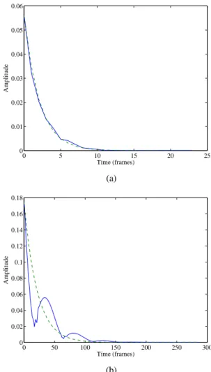
For each mode, some peaks whose frequencies are close to the frequency of the mode are tracked over time using standard frequency proximity criterion [9] to form modal tracks. Figure 4 shows the evolution of the amplitude of two modal tracks through time. For a given track, the amplitude is expressed as the evolution of the amplitudes estimated during the broad-band analysis (solid line), as a function of the damping values measured (dotted line), or as a function of the median value of the damping values over the entire duration of the modal track (dashed line).
Depending on the cases, the fit obtained after the initial mod-eling can be as good as on top of Figure 4(a) or as bad as on Fig-ure 4(b), where the beating clearly indicates the presence of more than one mode at this frequency. In cases similar to the latter, fur-ther analysis is then required to achieve a better estimation of the model.
5. FOCUSED ANALYSIS STEP
Before starting the second analysis we perform a selection of the partial tracks to process. First of all, the modal tracks with too low an amplitude (< −60dB) and that are too short (≈ less than 10 frames) are discarded from the focused analysis. Then, we com-pute the mean error between the amplitude of the modal track and the estimated amplitude profile (computed using the median es-timated damping value). If this error is above a given threshold, we decide to perform the second step of the modal analysis: a preprocessing step followed by either ARMA modeling, or a non-adaptive ESPRIT analysis.
5.1. Pre-Processing
In order to focus the analysis on the selected modal track, the sig-nal is bandpass filtered with a complex FIR filter centered around the median of the estimated frequencies over the whole track. Then this signal is modulated and down-sampled before being fed to the parametric spectral estimation method. One of the main in-terests of this step is to restrict the possible value of the order of
0 5 10 15 20 25 0 0.01 0.02 0.03 0.04 0.05 0.06 Time (frames) Amplitude (a) 0 50 100 150 200 250 300 0 0.02 0.04 0.06 0.08 0.1 0.12 0.14 0.16 0.18 Time (frames) Amplitude (b)
Figure 4: Evolution of the Amplitude over time. A strong correla-tion between the measured amplitude and the one computed using the damping parameter can be observed on (a) and not on (b).
the model. Indeed, by using a complex filter, we make sure only to consider positive frequencies, thus dividing the necessary order by two. Moreover, by only considering a narrow sub-band of the spectrum we limit the number of potential components to identify.
5.2. Auto-Regressive Analysis
Here we use the Steiglitz-McBride ARMA estimation method [10] to identify the frequencies and damping factors of the model. Us-ing an AR order K and a MA order p, we analyze the pre-processed signal. The K poles, zkof the sound are computed by finding the
roots of the AR part of the signal model. The frequency and damp-ing factor of the mode associated to one of these poles is obtained as follows:
fk=
=(log (zk))
2π and δk= <(log (zk)) (2) where M is the down-sampling factor and fcis the frequency of
5.3. High-Resolution Analysis
The other option we chose for the second pass of analysis is to use the ESPRIT algorithm on the pre-processed signal. Here we use a non-adaptative version of ESPRIT and thus treat the modal track on its entire duration. The pre-processing guarantees that the signal to process has a reasonable size (not more than 1000 samples [11]). The analysis parameters are the model order K and the “pencil parameter", i.e. the number of data vectors used to construct the approximation of the autocorrelation matrix. Based on the theoretical analysis presented in [12], we set p to the optimal value ofN +13 where N is the size of the down-sampled, modulated modal track.
5.4. Sorting the results
Once the frequencies and damping factors are estimated for all the components of the model, the amplitudes and phases are estimated via least squares estimation based on the input signal.
The last part of this analysis consists in discarding the irrele-vant components. This is done by discarding components which would diverge (δk > 0) and those with frequencies too far from
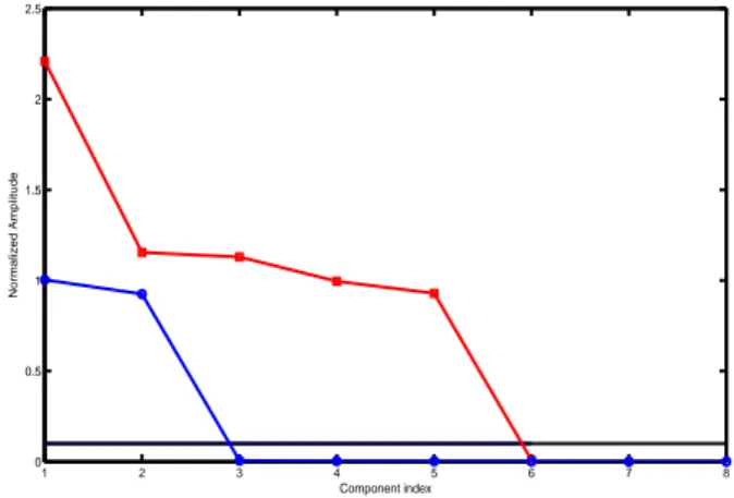
the median of the modal track frequencies. Finally, we only keep components with amplitudes within a given threshold of the max-imum amplitude of the modal track, see Figure 5.
6. EXPERIMENTS
The proposed scheme for modal analysis was implemented in Mat-lab. The implementation details of this framework are presented. The performance of different configurations of the two steps is evaluated over synthetic data. Finally, we show how this new tool can be applied to real life scenarios.
6.1. Modal Analysis Framework
As detailed in the previous sections, the proposed analysis scheme has two main steps: the broad-band analysis step and the focused analysis step. The first one is implemented using whether a Fourier based analysis or the High Resolution analysis method1.
The Fourier based analysis is implemented using the phase vocoder approach for the estimation of the frequency and the am-plitude is further refined using this frequency estimate [7]. A win-dow size of ≈ 0.1s and a hop size of ≈ 1.5ms is considered. A maximum of 180 sinusoidal components can be detected per frame. The HR analysis is parametrized equally except for the window size which is twice the hop size.
Once the modes are identified and tracked as described in Sec-tion 4 with an identificaSec-tion threshold at 10 dB, the focused analy-sis is performed in the frequency region of the identified modes.
The ARMA analysis was performed using K = 8 and p = 4 as was suggested in [13]. For the HR analysis, the order of the model was K = 8. The frequency range was set to 0.001 normal-ized frequency wide and the amplitude threshold was set to 0.1. 6.2. Performance over Synthetic Data
In order to illustrate the behaviors of the different possible analysis scenarios, the following methodology is considered. One thousand synthetically generated sets of modes are used to each synthesize
1The Matlab code is available upon request to R. Badeau
1 2 3 4 5 6 7 8 0 0.5 1 1.5 2 2.5 Component index Normalized Amplitude
Figure 5: Normalized amplitude of the components estimated us-ing the ARMA (square) and the HR (circle) focused analysis meth-ods in the case of a test signal consisting of two closely spaced modes. Only the components with amplitude higher than the threshold (solid line) are considered.
one second of sound. The amplitudes are randomly chosen in the (0.9, 1) range, the damping factors in the (0.0001, 0.001) range.
Two different frequency distributions are considered in two different experiments. In the first one, only two modes are consid-ered within a small frequency range (0.2499, 0.2501) in normal-ized frequency. In the second distribution, 20 modes are generated within the (0.2, 0.3) normalized frequency range.
The different combinations of broad-band and focused analy-sis methods are then considered to estimate modes from the syn-thetic sound file. The original set of modes and the estimated one are then compared to evaluate the performance of a given analysis scheme using the following criterion:
c = 10 log10 „ P sori(n)2 P(sori(n) − sest(n))2 « (3) where sori(n) and sest(n) are respectively the signal generated from
the original set of modes and the estimated one, using Equation 1 over 1 second, with initial phases equal to 0.
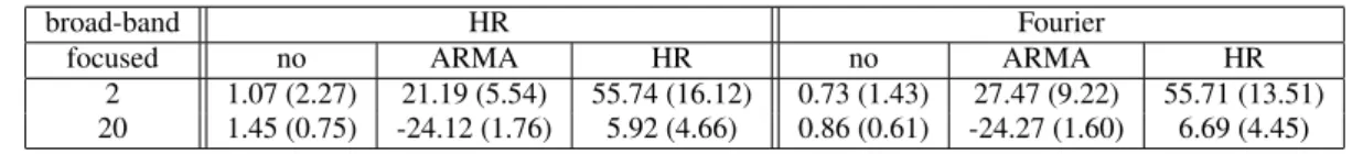
The first experiment shows the behavior of the proposed ap-proaches when facing closely spaced sinusoids. The sole use of the broad-band analysis step is not sufficient to distinguish between very close partials leading to an equivalent result for the Fourier and HR approaches, see Table 1. The use of the focused analy-sis allows us to distinguish the two modes leading to a significant improvement. The ARMA approach tends to consistently over es-timate the number of components due to a difficult thresholding of the amplitude of the detected components, see Figure 5, leading to inferior performance compared to the HR focused analysis.
The second experiment considers a modal distribution closer to the one of percussive sounds. The sole use of the first step gives consistent results. The overestimation of the number of modes within a focused analysis makes the ARMA perform badly, whereas the use of the HR focused analysis provides a significant improve-ment. A similar performance is achieved whether we use the HR or Fourier broad-band analysis followed by the HR focused analysis. This leads us to the conclusion that, for our purpose, an efficient
broad-band HR Fourier
focused no ARMA HR no ARMA HR 2 1.07 (2.27) 21.19 (5.54) 55.74 (16.12) 0.73 (1.43) 27.47 (9.22) 55.71 (13.51) 20 1.45 (0.75) -24.12 (1.76) 5.92 (4.66) 0.86 (0.61) -24.27 (1.60) 6.69 (4.45)
Table 1: Performance of the different analysis schemes. Mean and (standard deviation) of c are computed over 1000 realizations.
Fourier-based broad-band analysis followed by a HR focused anal-ysis over some frequency regions is the most appropriate approach. 6.3. Application to the Estimation of Excitation Signals One can perform a deconvolution of a sound with the impulse re-sponse of a filter identified by modal analysis. In a Source/Filter modeling paradigm this allows to estimate the source (a.k.a. exci-tation).
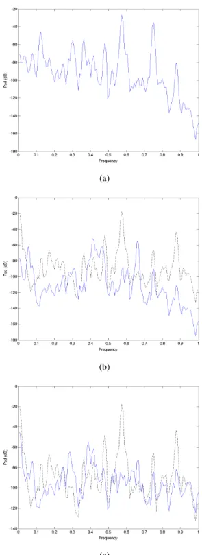
We consider here two sounds, one from a plucked classical guitar, and one from a metallic plate struck by a ceramic hammer. The power spectral density (PSD) of the two sounds and the PSD of the excitation signals with and without focused analysis are rep-resented in Figures 6 and 7. For these examples, we applied the HR based broad-band analysis only and the Fourier based broad-band analysis followed by the two flavors of focused analysis. We then used the standard inverse filtering approach presented in [1] to es-timate the excitation based on the modal parameters eses-timated.
In general, we can see that the main modes of the original sounds are more consistently absent of the excitation signal after the focused analysis steps. We note the presence of some rela-tively strong modes for example in Figure 6 (c) at frequency 0.05 or in Figure 7 (b) at frequency 0.65. These are actually artifacts of the deconvolution process (see [14] for some solutions to that problem). Comparing ARMA and HR focused analysis we ob-serve that the excitation PSDs obtained using HR focused analysis exhibit a generally flatter spectrum with more energy in the high frequencies, consequence of a shorter duration of the actual ex-citation signal and thus, would seem more adapted for efficient parametrization of a percussive sound.
7. ACKNOWLEDGMENTS
The authors would like to thank Roland Badeau for kindly pro-viding us with the HR analysis method considered for broad-band analysis. This work was supported by a Special Research Oppor-tunity grant from the Natural Sciences and Engineering Research Council of Canada.
8. CONCLUSION
A two-step analysis scheme for the estimation of modal parame-ters from recorded sounds has been proposed. It aims at alleviat-ing the tedious parametrization and manual post-processalleviat-ing usu-ally needed when only one analysis step is considered.
A broad-band analysis is processed over the entire duration of the signal allowing to gain some insight about the time/frequency regions of interest. Focusing on those regions, the second step is able to reliably identify modes and estimate their parameters even in the case of closely-spaced components.
The interest of this two-step modal identification approach was demonstrated for synthetic data as well as in the real scenario of excitation signal estimation in source filter modeling.
9. REFERENCES
[1] J. Laroche and J. L. Meillier, “Multichannel excitation/filter modeling of percussive sounds with application to the piano,” IEEE Trans. on Speech and Audio Processing, vol. 2, no. 2, pp. 329–344, April 1994.
[2] K. van den Doel, P. G. Kry, and D. K. Pai, “FauleyAutomatic: physically-based sound effects for interactive simulation and animation,” in Proc. ACM SIGGRAPH, Los Angeles, CA, USA, Aug. 12-17 2001, pp. 537–544.
[3] S. M. Kay, Modern Spectral Estimation, chapter Autore-gressive Spectral Estimation : Methods, pp. 228–231, Sig-nal Processing Series. Prentice Hall, Englewood Cliffs, NJ, USA, 1988.
[4] R. Badeau, G. Richard, and B. David, “Fast adaptive ESPRIT algorithm,” in Proc. IEEE Workshop on Statistical Signal Processing, Bordeaux, France, Jul. 17-20 2005, pp. 289–293. [5] R. Badeau, High Resolution Methods for the Estimation and the Tracking of Modulated Sinusoids. Application to musical signals., Ph.D. thesis, Telecom Paris, 2005, in French. [6] A. H. Benade, Fundamentals of Musical Acoustics, Dover,
New York, NY, USA, 2nd edition, 1990.
[7] M. Lagrange and S. Marchand, “Estimating the instan-taneous frequency of sinusoidal components using phase-based methods,” to appear in J. of the Audio Eng. Soc., 2007. [8] R. Roy, A. Paulraj, and T. Kailath, “ESPRIT – a subspace rotation approach to estimation of parameters of cisoids in noise,” IEEE Trans. on Acoustics, Speech, Signal Processing, vol. 34, no. 5, pp. 1340–1342, October 1986.
[9] R. J. McAulay and T. Quatieri, “Speech analysis/synthesis based on a sinusoidal representation,” IEEE Trans. on Acous-tics, Speech, and Signal Processing, vol. 34, no. 4, pp. 744– 754, August 1986.
[10] K. Steiglitz and L.E. McBride, “A technique for the identifi-cation of linear systems,” IEEE Trans. on Automatic Control, vol. 10, no. 4, pp. 461–464, October 1965.
[11] J. Laroche, “The use of the matrix pencil method for the spectrum analysis of musical signals.,” J. Acoust. Soc. Am., vol. 94, no. 4, pp. 1958–1965, October 1993.
[12] Y. Hua and T. Sarkar, “Matrix pencil method for estimating parameters of exponentially damped/undamped sinusoíds in noise.,” IEEE Trans. on Acoustics, Speech, Signal Process-ing, vol. 38, no. 5, pp. 814–824, May 1990.
[13] M. Karjalainen and T. Paatero, “High-resolution paramet-ric modeling of string instrument sounds,” in Proc. of EU-SIPCO, Antalya,Turkey, Sept. 4-8 2005, pp. CD–ROM pro-ceedings.
[14] M. Lagrange, N. Whetsell, and P. Depalle, “On the control of the phase of resonant filters with applications to percussive sound modelling,” in Proc. Digital Audio Effects (DAFx-08), 2008.
(a)
(b)
(c)
Figure 6: Normalized Power Spectral Density of a guitar sound (a) and the corresponding estimated excitation using a HR band analysis only (dashed line) and in solid line, a Fourier broad-band analysis followed by, respectively, the ARMA focused analy-sis (b), and the HR focused analyanaly-sis (c).
(a)
(b)
(c)
Figure 7: Normalized Power Spectral Density of a plate hit by a hammer (a) and the corresponding estimated excitation using a HR broad-band analysis only (dashed line) and in solid line, a Fourier broad-band analysis followed by, respectively, the ARMA focused analysis (b), and the HR focused analysis (c).