HAL Id: hal-02389078
https://hal.inria.fr/hal-02389078
Submitted on 10 Dec 2019
HAL is a multi-disciplinary open access
archive for the deposit and dissemination of
sci-entific research documents, whether they are
pub-lished or not. The documents may come from
teaching and research institutions in France or
abroad, or from public or private research centers.
L’archive ouverte pluridisciplinaire HAL, est
destinée au dépôt et à la diffusion de documents
scientifiques de niveau recherche, publiés ou non,
émanant des établissements d’enseignement et de
recherche français ou étrangers, des laboratoires
publics ou privés.
Incorporating Probabilistic Optimizations for Resource
Provisioning of Data Processing Workflows
Amelie Chi Zhou, Yao Xiao, Bingsheng He, Shadi Ibrahim, Reynold Cheng
To cite this version:
Amelie Chi Zhou, Yao Xiao, Bingsheng He, Shadi Ibrahim, Reynold Cheng. Incorporating
Prob-abilistic Optimizations for Resource Provisioning of Data Processing Workflows.
ICPP 2019
- 48th International Conference on Parallel Processing, Aug 2019, Kyoto, Japan.
pp.1-10,
Incorporating Probabilistic Optimizations for Resource
Provisioning of Data Processing Workflows
Amelie Chi Zhou
1Yao Xiao
1Bingsheng He
2Shadi Ibrahim
3Reynold Cheng
41Shenzhen University2National University of Singapore3Inria, IMT Atlantique, LS2N4The University of Hong Kong
ABSTRACT
Workflow is an important model for big data processing and resource provisioning is crucial to the performance of workflows. Recently, system variations in the cloud and large-scale clusters, such as those in I/O and network performances, have been observed to greatly affect the performance of workflows. Traditional resource provisioning methods, which overlook these variations, can lead to suboptimal resource provisioning results. In this paper, we provide a general solution for workflow performance optimizations consid-ering system variations. Specifically, we model system variations as time-dependent random variables and take their probability distributions as optimization input. Despite its effectiveness, this solution involves heavy computation overhead. Thus, we propose three pruning techniques to simplify workflow structure and reduce the probability evaluation overhead. We implement our techniques in a runtime library, which allows users to incorporate efficient probabilistic optimization into existing resource provisioning meth-ods. Experiments show that probabilistic solutions can improve the performance by 51% compared to state-of-the-art static solutions while guaranteeing budget constraint, and our pruning techniques can greatly reduce the overhead of probabilistic optimization.
KEYWORDS
Resource provisioning, Cloud dynamics, Workflows
1
INTRODUCTION
In many data-intensive applications, data processing jobs are often modeled as workflows, which are sets of tasks connected according to their data and computation dependencies. For example, Montage workflow [20] is an astronomy-related big data application, which processes sky mosaics data in the scale of hundreds of GBs. Large companies such as Facebook, Yahoo, and Google frequently execute ad-hoc queries and periodic batch jobs over petabyte-scale data based on MapReduce (MR) workflows [30]. Those data-intensive workflows are usually executed in large scale systems and resource provisioning, which determines the size and type of resources to execute workflow tasks, is important to the performance of workflows and has been widely studied by existing work [14, 15, 18]. In many large-scale systems, variations have become the norm rather than the exception [8, 27]. Variations can be caused by both hardware and software reasons. For example, in supercomputer architectures, the variation in power and temperature of the chips can cause up to 16% performance variation between processors [1]. In cloud environments, network and I/O performances also show significant variations due to user interferences [27]. Job failures have been demonstrated to be variant and follow different kinds of probability distributions for different systems [8]. These variations, which have been ignored by most existing optimization methods,
raise new challenges to the resource provisioning problem of workflows. In this paper, we focus on the cloud system, aiming at proposing a general solution to incorporating system variations for resource provisioning problems of workflows.
Why consider variations? Cloud providers offer various types of instances (i.e., VMs) for users to select the most appropriate resources to execute workflow tasks. Most existing resource pro-visioning methods assume that the execution time of each task is static on a given type of VMs. However, this assumption does not hold in the cloud, where cloud dynamics, such as the variations of I/O and network performances, can result in major performance variation [22, 27] to large-scale data processing workflows. We analyzed several common resource provisioning problems for workflows, and observed that the performance optimization goal is usually nonlinearly related to the cloud dynamics in I/O and network performance. Thus, traditional static optimizations (e.g., taking the average or expected I/O and network performance as optimization input) can lead to suboptimal or even infeasible solutions (theoretically explained in Section 3).
Why probabilistic method? Existing studies propose various methods such as dynamic scheduling [10, 15] and stochastic model-ing [2, 11] to address resource provisionmodel-ing problems considermodel-ing cloud dynamics. However, these methods either rely on accurate cloud performance estimation at runtime or involve complicated modeling and analysis and thus hard to generalize. For example, Adam et al. [2] employ the G/G/m queuing model for resource provisioning of containerized web services in clouds, and Huang et al. [11] address spot price dynamics based on Markov decision processes. In this paper, we study a systematic and effective way of incorporating cloud dynamics into resource provisioning of work-flows. We model cloud dynamics as random variables and take their probability distributionsas optimization input to formulate resource provisioning problems. This design has two main advantages. First, it enables probabilistic analysis required by many problems with system randomness, such as designing fault-tolerant scheduling techniques for workflows in case of random system failures [25]. Second, it enables the derivation of probabilistic bounds [26] to guarantee the worst-case performance of applications, while the existing static methods only guarantee the average performance.
Why this paper? With the probabilistic representation of cloud dynamics, traditional static resource provisioning methods cannot be used directly. The main challenge is that using probability distributions as optimization input leads to a significantly high computation overhead due to the costly distribution calculations and complex structures of data processing workflows. There exist some techniques to improve the efficiency of probabilistic optimization in various fields, such as efficient query evaluations in probabilistic databases [5], accurate data processing with uncertain data [16]
and efficient probabilistic cluster scheduling with runtime uncer-tainty [23]. However, these techniques either rely on given proba-bility distributions [16] or do not consider the special features of workflow structure and resource provisioning problems [23], which can help to more efficiently reduce the overhead of probabilistic resource provisioning of workflows.
Contributions: We propose Prob to efficiently incorporate cloud dynamics into resource provisioning for workflows, without any assumption on the distribution of cloud dynamics. Prob has three simple yet effective pruning techniques to reduce the overhead of probabilistic optimizations. These techniques are designed based on features of workflow structures and resource provisioning problems. First, we identify that calculating the makespan of a workflow is a common operation in many resource provisioning problems. We propose pre-processing pruning to reduce the overhead of this important calculation and hence reduce the overhead of probabilistic optimizations. Second, we propose workflow-specific optimizations using existing workflow transformations to reduce the overhead of evaluating one resource provisioning solution. Third, we propose a partial solution evaluation method and adopt an existing pruning technique to reduce the overhead of comparing multiple solutions.
We develop a runtime library that includes all the pruning techniques of Prob. Users can implement their existing resource provisioning methods using Prob APIs to incorporate probabilistic optimizations, in order to improve both the effectiveness and efficiency of existing methods. We experimented with real-world workflows on Amazon EC2 and with simulations to show the effec-tiveness of probabilistic optimizations and our pruning techniques. Our experiments demonstrate up to 51% performance improvement of probabilistic solutions compared to state-of-the-art static solutions. The pruning techniques of Prob bring significant reduction to the overhead of probabilistic solutions (e.g., 450x speedup compared to the Monte Carlo (MC) method).
Goals and non-goals: Our goal is to propose an efficient interface for existing resource provisioning methods to easily incorporate probabilistic optimizations, rather than proposing a new resource provisioning method. To show the generality of Prob, we use a common workflow resource provisioning problem as use case and discuss how Prob can improve the effectiveness of existing solutions.
2
PRELIMINARIES
2.1
Data Processing Workflows
A data processing workflow (a job) can be described as a directed acyclic graph (DAG) [7]. A vertex in the DAG represents a task in the workflow while an edge represents the data dependency between two tasks. A task in a workflow performs certain data transformation to its input data. We adopt an existing approach [31] widely used for data-intensive task execution time estimation, which calculates the task execution time as the sum of the CPU, I/O and network time. We define a virtual entry vertex and a virtual exit vertex in a workflow. The entry vertex does nothing but staging input data of the workflow while the exit vertex saves output results.
Resource provisioning for a workflow in the cloud decides the number and types of cloud instances required for executing the workflow. Performance is an important optimization metric for resource provisioning of data-intensive workflows and can be highly affected by resource provisioning decisions. Various methods have
(a) I/O performance of m1.large (b) I/O performance
(c) Network performance (d) I/O perf. of m1.large in Sep.
Figure 1: Cloud dynamics features observed on Amazon EC2.
(a) I/O performance (b) I/O performance of A1
Figure 2: Cloud dynamics features on Windows Azure. been proposed to optimize either the performance of workflows in the cloud [8, 18] or the monetary cost/energy efficiency of workflows with performance constraints [12, 14, 15].
2.2
Cloud Dynamics Terminology
In this paper, we study two kinds of variations, namely the I/O and network performance variations, which are common in the cloud and decisive to the performance of workflows (the CPU performance is rather stable in the cloud [27]). We extend the analysis to other system variation factors in our technical report [33]. Formally, we define the I/O (network) performance dynamics as below.
DEFINITION1. We view the I/O (network) bandwidth assigned to a running task as a random variable (r.v.)X . The I/O (network) bandwidth dynamics can be described with a probability distribution (PDF)fX(x), which represents P(X = x).
The above definition greatly changes the formulation and solving of resource provisioning problems for workflows in the cloud. Consider a simple example of calculating the expected I/O time of a task. With the static definition of I/O bandwidth as a scalar value bio(bio = Íxx · fX(x)), we have tio= dbioio, wherediois the I/O data volume of a task andtiois the I/O time. With our definition of I/O bandwidth dynamics, the value oftiois also dynamic. Defining the I/O time of the task with r.v.T , we can use the PDF of I/O bandwidth to calculate the distribution ofT as fT(t) = fX(diot ). The expected value ofT is Íxdxio ·fX(x) and can be different from the result of the static method (i.e.,Í dio
xx ·fX(x)).
2.3
Features of Cloud Performance Dynamics
We study the spatial and temporal features of cloud performance dynamics in I/O and network. We demonstrate that the probability distributions of performance dynamics are predictable in a short period of time. We conduct the experiments on Amazon EC2 cloud. More details about the measurements can be found in Section 5.
Spatial features. The performance of instances of the same type can be modeled with similar/the same probability distributions. Figure 1a shows the distributions of the sequential I/O performances of four m1.large instances running on the same day, which follow very similar distributions. We performed the measurements on over 100 instances and found consistent results.
Another observation is that, the probability distributions of performances of different types of instances usually have similar patterns with different parameters. Figure 1b and 1c show the sequential I/O and network performance distributions of four instance types, respectively. For each type, data are collected from multiple instances over 1 day. The distributions have similar patterns with different mean and variances. For example, the mean network bandwidth is higher on more expensive instance types such as m1.large and m1.xlarge and the performance variance is more severe on cheap instance types such as m1.small and m1.medium.
Temporal features. The probability distributions of the cloud performance are stable within a short time period. Figure 1d shows the sequential I/O performance distributions of m1.large instances measured on the 9th, 10th, 14th and 15th September, 2015, where distributions in a short period of time are closer to each other in terms of mean and variance. Quantitatively, we adopt the Bhattacharyya distance[3], a commonly used statistical metric, to measure the similarity of two distributions (smaller distance indicates higher similarity). The distance between the I/O performance distribution of the 9th and that of the 10th is only0.03, while the distance between the distributions of the 9th and the 14th is0.1. This means that the I/O performance distribution in a short period of time (e.g., one day) is more stable than that in a longer period (e.g., five days). The same observation has also been found on the network performances.
To demonstrate the generality of our observations, we perform similar experiments on Windows Azure using three general purpose instance types, namely A0, A1 and A2. Figure 2a demonstrates that the spatial feature can also be observed on Azure, where distributions of the sequential I/O performance of different instance types follow similar patterns with different parameters. A1 has higher performance variation than the other two types. We suspect it is because A1 is the recommended type of Azure and thus has more users. Figure 2b shows that the temporal feature also holds on Azure, where the I/O performance distribution of A1 measured in Day 1 is more similar to that of Day 2 than that of a longer period in Day 7. Summary: The spatial and temporal predictability of cloud dynamics verifies that it is feasible to represent cloud dynamics using their distributions and adopt probabilistic methods to optimize the resource provisioning problems.
3
PROBABILISTIC APPROACH IS NEEDED
As a motivating example, we present a common resource provision-ing problem for workflows in the cloud. We first present an existprovision-ing solution [32] to this problem under static performance notions and then discuss our solution considering cloud dynamics. We show that cloud dynamics can greatly affect the optimization effectivenesses. All the mathematical proofs can be found in our technical report [33].
3.1
Budget-Constrained Scheduling Problem
Cloud providers offer multiple instance types with different capabili-ties and prices. In this problem, we aim to select a suitable instance
type for each task in a workflow to minimize workflow execution time while satisfying budget constraint.
Consider a workflow withN tasks running in a cloud with K types of instances. The optimization variable of this problem is vmij, meaning assigning instance typej (j = 0, 1, . . . , K − 1) to task i (i = 0, 1, . . . , N − 1). The value of vmijis1 (i.e., taski is assigned to instance typej) or 0 (otherwise). We denote the execution time of taski on instance type j using r.v. Tijwith a probability distribution fTi j(t). We denote the workflow execution time (i.e., makespan)
with r.v.Twand calculate its distributionfTw(t) using the execution
time distributions of tasks on the critical path (denoted asCP). The user-defined budget constraint is denoted asB, which includes the instance rental cost and networking cost. The unit time rental price of instance typej is denoted as Uj. The networking cost of taski transferring data to its child tasks is denoted asCneti .E[X ] denotes the expected value of a r.v.X . We formulate the problem as below.
minE[Tw]= min E[Õ
j Õ i ∈C P Ti j×vmi j] (1) s.t. Õ i{ Õ jE[Ti j] ×vmi j×Uj+ C i net} ≤B (2) Õ jvmi j= 1, ∀i ∈ 0, . . . , N − 1 (3)
3.2
A Static Solution
The budget-constrained scheduling problem has been widely stud-ied [14, 18] using either heuristics or model-based methods. However, most of them assume static task execution time during the optimization. We first introduce a traditional static approach for the budget-constrained scheduling problem, and discuss how to incorporate cloud dynamics next.
We adopt an existing method [32] which formulates resource provisioning problems as search problems, and adopt generic search or more efficientA⋆search to find a good solution. We choose this algorithm for its generality. We briefly present the behavior of the search algorithm as below (see also Algorithm 1).
A states in the solution space is modeled as a N -dimensional vector, wheresi stands for the instance type assigned to taski. Correspondingly,vmij equals to 1 if j = si and 0 if otherwise. It searches the solution space in a BFS-like manner. Each found solution is evaluated using Equation 1 for the optimization goal and Equation 2 for the budget constraint. The static optimizations take the expected I/O and network performance as input to estimate the task execution time. That means,Tijis only a scalar value and computing Equation 1 and 2 is light-weight. After evaluating a solution, we compare it with the best found solution and keep the one with better evaluation result while meeting the constraint. The search process terminates if the entire solution space has been traversed or a pre-defined number of iterations has been reached.
3.3
A Probabilistic Method
To incorporate cloud dynamics into the static method, we have made two efforts. First, we take the I/O and network performance dynamics of instance typej to estimate the probability distribution of Tij. Second, wheneverTijis used in the search process, we perform probabilistic calculations on distributions, e.g., adding task execution time distributions to obtain path execution time distribution, finding the maximum execution time distribution of multiple paths (i.e., finding the critical path) to evaluate the optimization goal in
Figure 3: An example of probabilistic optimizations. Equation 1, and comparing evaluation metric distributions of two found solutions to find a good solution.
The distribution addition with two independent r.v., e.g.,Z = X + Y, can be calculated as below.
fZ(z) = ∫ ∞
−∞
fY(z − x)fX(x) dx (4)
Finding the maximum distribution of two independent r.v., e.g., Z = max{X,Y }, can be calculated as below. FX(x) and FY(y) are the cumulative distribution functions (CDFs) ofX and Y , respectively.
fZ(z) = d
dzFY(z)FX(z) = FY(z)fX(z) + FX(z)fY(z) (5)
We adopt the following definition to compare two evaluation metric distributions. Given two independent r.v.X and Y , we have X > Y if P(X > Y ) > 0.5, where P (X > Y ) = ∫ ∞ −∞ ∫ ∞ y fX(x)fY(y) dx dy (6)
Figure 3 gives a concrete example to show the difference between static and probabilistic optimizations. Consider the budget-constrained scheduling for a workflow with four tasks. The execution time distributions of tasks have been calculated using I/O and network performance distributions, as shown in the table. There are2 paths in the workflow. To optimize workflow performance, we need to identify the critical path and schedule tasks on the critical path to more powerful VMs. We make the following observations.
Probabilistic optimization is more effective. With the tradi-tional static method, the expected lengths of edges are used for evaluations and path2 is returned as the critical path with a length of251.5. With our probabilistic method (introduced in details in Section 4), we first calculate the length distributions of the two paths and then calculate the maximum of the two distributions. Given the length distributions of path 1 and 2 (denoted as ®T1and ®T2,
respectively), the expected length of the critical path is257.4. The probability of path2 being the critical path is only 0.48. Theoretically, this observation is supported by the following lemma, which shows that for parallel structured workflows, static methods using average task execution time as input always under-estimate the expected workflow execution time.
LEMMA1. Given two independent r.v.X and Y , for the r.v. Z = max{X, Y }, we have E[Z] ≥ max{E[X ], E[Y ]}.
For workflows with complex structures, the estimation errors of static methods can accumulate and lead to more inaccurate or even incorrect optimization results. Consider the above example with a workflow structured as two of the same workflow in Figure 3 standing in parallel. The expected workflow execution
time calculated using the static and probabilistic methods are251.5 and271.6, respectively. Thus, the under-estimation problem is more severe for workflows with complex structures and it is important to consider cloud dynamics for resource provisioning of workflows.
Probabilistic optimization is costly. A straight-forward way to implement probabilistic optimization is to use the sampling-based Monte Carlo (MC) approach, which calculates all possible results using input probability distributions. For example, to obtain the sum distribution of Equation 4, we performM times of MC calculations. In each calculation, we randomly sample values from the discretized distributions fX(x) and fY(y) to get a possible result of the sum. After theM times calculations, we can create the sum distribution using theM calculated sum results. Thus, the time complexity of adding two task execution time distributions isO(M) and for adding n tasks is O((n − 1)M). Note that M is usually very large to achieve good accuracy. For a workflow with complex structure and a large number of tasks, the time complexity for calculating the workflow execution time distribution is high. Similarly, with the MC approach, the time complexity of calculating the maximum distribution is O(M) and of comparing two evaluation metric distributions is O(M2).
Thus, the computation overhead of probabilistic optimization is prohibitively high due to the largeM, complex workflow structures and costly distribution comparisons.
In summary, probabilistic distributions improve the effectiveness of workflow optimizations in dynamic clouds while causing a large overhead. This motivates us to develop an effective and efficient approach for resource provisioning of workflows in the cloud.
4
DESIGN OF PROB
We propose a probabilistic optimization approach named Prob for incorporating cloud dynamics into workflow optimizations. We introduce three simple yet effective pruning stages in Prob to address the large overhead of probabilistic optimizations caused by complex workflow structures and costly calculations and comparisons of distributions. First, calculating the makespan of a workflow is a common operation in many resource provisioning problems of workflows. Thus, we propose pre-processing pruning to reduce the overhead of this important calculation and hence reduce the overhead of probabilistic optimizations. This stage is an offline optimization stage, as a workflow only needs to be optimized once and for all. Second, we propose workflow-specific optimizations using existing workflow transformation techniques to reduce the overhead of evaluating one resource provisioning solution. Third, we propose two pruning techniques to reduce the overhead of comparing multiple solutions. The latter two stages are called at the runtime of solution search process.
4.1
Pre-Processing
Calculating the execution time of a workflow is a common operation in many resource provisioning problems of workflows. Due to cloud dynamics, the execution time of a workflow is represented as a random variable. To obtain its probability distribution, we first decompose a workflow into a set of paths starting from the entry to the exit task of the workflow. The execution time distribution of the workflow is the maximum of execution time distributions of all paths in the set. We further propose a critical path pruning and a path binding technique to reduce the number of paths in the set and hence reduce the overhead of calculating workflow
Figure 4: Example of pre-processing using Montage workflow. execution time distribution. In Figure 4, we use the structure of a real-world scientific workflow named Montage [24] to demonstrate the effectiveness of the two pruning techniques.
Given a workflow, we can easily enumerate all paths in the workflow using depth-first search inO(2V) time, whereV is the number of vertices in the workflow. Although the exponential time complexity is not ideal, the pre-processing optimization is at offline time and only has to be performed once for a given workflow structure. The pre-processing results can be used for all further optimization problems of the same workflow structure. Assume all paths from the entry task to the exit task are stored in a setS. We introduce the following two techniques to reduce the size ofS.
Critical Path Pruning. This technique eliminates the paths that are impossible to be the critical path fromS. For example, in Figure 4, as the execution time of pathP2must be shorter than that ofP1,
clearlyP2is not the critical path. Similarly, pathP48is impossible to
be the critical path due toP47. We can eliminate such paths fromS
and reduce the size ofS from 48 to 44. We denote the set of paths after pruning asS′.
The critical path pruning follows the following rule: given any two pathsP1 andP2between the entry and exit tasks of a DAG,
if the set of nodes inP1 is a subset of that in P2,P1 is not the
critical path. We order all paths inS according to their lengths, and iteratively compare the longest path with the ones shorter than it using the above rule. The expected time complexity of this technique isO(|S |ln|S | × L), where L is the average length of paths in S.
Path Binding. GivenS′in Figure 4, we need in total352 distri-bution additions to evaluate path distridistri-butions and43 distribution maximum operations to obtain workflow execution time distribution. However, we find that when evaluatingP1′andP2′separately, many of the distribution additions are repetitive. By bindingP1′ with P′
2, we can reduce the overhead from 16 distribution additions
to8 distribution additions and one operation on calculating the maximum distribution of task 4 and 5. We can apply the binding to all paths inS′and reconstruct them to a single path as shown inS′′. WithS′′, the overhead of calculating the workflow execution time distribution is reduced to8 distribution additions and 11 distribution maximum operations. As the distribution addition and maximum operations have the same time complexity with the MC method, path binding reduces the overhead of calculating workflow execution time distribution by 95%.
Formally, the path binding technique binds two paths with the same lengthL in the following way. We compare each node of one path with the node in the same position of the other path in order. If thei-th nodes (i = 0, . . . , L − 1) are the same, they are adopted as the i-th node of the binded path. Otherwise, we bind the i-th nodes of the paths as one node, the execution time of which is the maximum of thei-th nodes of the two paths. Assume there are k binded nodes in the binded path, the calculations saved by binding the two paths isL − k − 1. We iteratively select two paths in S′with the best gain to bind until no gain can be further obtained or the largest number of iterations have been reached. This technique is especially useful for data processing workflows such as MR jobs, where the input data partitions go through the same levels of processing (i.e., all paths have the same length). The expected time complexity of this pruning isO(|S′|ln|S′| ×L), where L is the average length of paths in S′.
Note that the pre-processing only needs to be applied once at offline time and the results can be reused for different resource provisioning problems of the same workflow structure.
4.2
Workflow-Specific Optimizations
After the pre-processing stage, evaluating a found solution, namely calculating the execution time distribution of a workflow according to the instance configurations indicated by the solution, is simplified to calculating the distributions of several paths. The workflow execution time distribution is calculated as the maximum distribution of all path distributions.
We decompose the calculation of workflow execution time distribution to two constructive operations, namely ADD and MAX. The ADD operation can be applied to the distributions of two dependent tasks while the MAX operation can be applied to the distributions of two parallel tasks or two paths from the pre-processing result. We define ADD and MAX as binary operators, which operate on two probability distributions at a time. To apply ADDand MAX onn (n > 2) distributions, we perform the operators n − 1 times. For example, the execution time distribution of path P2
in Figure 4 can be calculated as
PDFP2=ADD(ADD(ADD(ADD(ADD(PDF0, PDF12), PDF16), PDF17), PDF18), PDF19) (7)
where PDFi denotes the execution time distribution of taski on the instance type assigned by the current evaluated solution.
The calculation of ADD and MAX operations are introduced in Equations 4 and 5, respectively. As discussed in Section 3, a straight-forward implementation for ADD and MAX is to use the sampling-based MC method. However, this implementation can lead to a large overhead due to complex workflow structures and the large sampling size. Thus, we adopt two existing workflow transformation optimiza-tions to reduce the overhead while preserving the correctness of ADDand MAX operations.
For many resource provisioning problems of workflows, existing studies have proposed various workflow transformations to simplify workflow structures, such as task bundling [17] and task cluster-ing[28]. Both operations attempt to increase the computational granularity of workflows and reduce the resource provisioning overhead. In this paper, we discuss the two operations from the perspective of probabilistic optimizations.
Optimizing ADD with task bundling. Task bundling treats two pipelined tasks with the same assigned instance type as one task, and
schedules them onto the same instance sequentially. For example, in Figure 4, we can bundle tasks10 and 11 inP1′′as one task when they have the same assigned instance type. Task bundling can increase instance utilization and reduce the amount of data transfer between dependent tasks. This technique gives us the opportunity to reduce the overhead of ADD operation.
When applying the ADD operation on two tasks, if the tasks satisfy the requirement of task bundling, we can directly generate the resulted distribution using the I/O and network profiles of the two tasks without calculating their distributions separately. With the naive MC implementation, the number of computations of the ADD operation is3M, which includes the computations for generating execution time distributions of two tasks and the computations for calculating the sum distribution.M is the number of MC calculations as mentioned in section 3.3. After applying task bundling, the number of computations of ADD is reduced toM.
Optimizing MAX with task clustering. In many data processing workflows, the data volume to be processed is huge. The execution is usually in a data parallel manner. Data are divided into a large number of partitions with equal sizes and are processed in parallel with many tasks. We denote those parallel tasks as equivalent tasks. In scientific workflows, tasks on the same level, using the same executable for execution and having the same predecessors are identified as equivalent tasks. In MR workflows, we can easily identify the map/reduce tasks on the same level as equivalent tasks. Task clustering groups two equivalent tasks assigned to the same instance type as one task and schedules them onto the same instance for parallel execution. For example, in Figure 4, tasks12 to 15 inP1′′ can be identified as equivalent tasks and grouped as one task with three times of clustering. Note that, the four tasks cannot be viewed as equivalent tasks before the pre-processing (e.g., inS and S′), since they have different predecessors. The task clustering technique offers opportunity to reduce the overhead of MAX operation.
As equivalent tasks have the same (or similar) resource require-ments and are executed on the same instance in parallel, we can use the execution time distribution of one of the equivalent tasks to represent the distribution of the clustered task. This can be verified with Lemma 1, whereE[max{X, Y }] = E[X] = E[Y] when X and Y are the same random variable. However, we must consider the performance degradation of the clustered tasks due to resource contention. Thus, when applying the MAX operation on two tasks, if they satisfy the requirement of task clustering, we usefX(x2) to represent the resulted distribution assumingfX(x) is the execution time distribution of one of the two tasks. With this optimization, we reduce the overhead of MAX fromO(M) to O(1). The number of equivalent tasks to be clustered is determined by the resource capacity of the instance and the resource requirement of tasks.
4.3
Distribution-Specific Optimizations
Given two resource provisioning solutions (i.e., two vectors of instance configurations for each task in the workflow), we evaluate each solution and compare their evaluation metric distributions to find a good solution. In the above, we have proposed to reduce the overhead of evaluating one solution. In this subsection, we mainly focus on reducing the overhead of solution comparisons to reduce the overhead of probabilistic optimizations. Specifically, we propose a partial solution evaluation technique and adopt an
existing pruning in probabilistic database to reduce the overhead of solution comparisons.
Partial solution evaluation. As the purpose of solution evalua-tions is to compare their quality and find a good one, we propose a partial solution evaluation technique to avoid fully evaluating two solutions while guaranteeing the same solution comparison result. When evaluating two solutionss and s′, we only calculate the distributions of tasks with different configurations ins and s′(i.e.,∀i wheresi , si′). Comparing the partially evaluated distribution ofs
with that ofs′gives the same result as comparing the fully evaluated distributions. This property is guaranteed by Lemma 2.
LEMMA2. Given two r.v.X and Y , assume X > Y . Then we have д(X, Z) > д(Y , Z) for any r.v. Z independent from X and Y , where д(·) is either ADD or MAX.
Consider two solutionss and s′for the workflow in Figure 4. Assumes differs from s′on the configurations of task10 and 11. With the partial evaluation,s′results in shorter workflow execution time thans if
P (ADD(PDF10s, PDFs11)> ADD(PDF10s′, PDFs11′))> 0.5 (8)
where PDFsi and PDFsi′are the execution time distributions of task i on the instance type assigned by s and s′
, respectively. In this way, we reduce the overhead of comparing the two solutions from38 probabilistic operations (either ADD or MAX) and one distribution comparison to two ADD and one distribution comparison.
Assume we visit in totaln solutions during the solution search process, the overhead of full solution evaluations would beO(n × (N −1)×M), where N is the number of tasks in a workflow. With our partial evaluation technique, assume the average number of different configurations in a pair of solutions isN′, the overhead of solution evaluations is reduced toO(2n × (N′− 1) ×M). For many resource provisioning algorithms, such as the search algorithm introduced in Section 3.2, adjacent solutions on the search tree only differ by a few configurations (i.e.,N′≪ N
2). Thus, partial solution evaluation
can greatly reduce solution search overhead. This pruning can be disabled when comparing two solutions where half of the tasks are assigned with different configurations.
Distribution comparison pruning. After solution evaluations (either partial or full), we repeatedly use Equation 6 for distribution comparisons during solution search process. The complexity of one distribution comparison isO(M2), which is extremely high due to the large sampling sizeM. Thus, we adopt an existing pruning technique [5] in probabilistic database to prune the unnecessary calculations of Equation 6. The basic idea is described as below.
Assume random variableX (resp. Y ) has the lower and upper bound ofX .l (resp. Y .l) and X .r (resp. Y .r), respectively. With Equations 9 and 10, we can estimate the lower bound or upper bound ofP(X > Y ). If the lower bound is greater than 0.5 or the upper bound is less than0.5, we can prune the calculation of Equation 6.
IfX .l ≤ Y .r ≤ X .r, P (X > Y ) ≥ 1 − FX(Y .r ) (9) IfX .l ≤ Y .l ≤ X .r, P (X > Y ) ≤ 1 − FX(Y .l) (10)
5
SYSTEM IMPLEMENTATION
Figure 5 shows the integration of Prob in existing data processing systems (e.g., Hadoop). We introduce two main design details of Prob. First, Prob stores system states (e.g., cloud performance
Figure 5: System overview
calibrations) and maintains the histograms (i.e., discrete distribu-tions) of cloud dynamics. Those distributions are taken as input by Prob-enabled system schedulers to find the optimal resource provisioning solution. Second, Prob offers a runtime library which exposes the probabilistic operations (e.g., ADD and MAX) and pruning techniques designed for resource provisioning problems of workflows. Existing schedulers of data processing systems can call the APIs in the library when implementing their resource provisioning methods to incorporate probabilistic optimizations. The data processing system schedules jobs to the cloud resources according to the optimized resource provisioning solutions.
5.1
Maintenance of Probability Distributions
As optimization inputs, we consider two types of system states, including 1) instance-related states such as price, CPU, I/O and network performances and 2) job-related states such as job start time and finish time. Prob collects those states from the cloud and maintains the data in an online and lightweight manner.
Data collection. System states are calibrated and updated period-ically. Instance-related states are measured from the cloud platform by opportunistically taking the idle time of running instances. As the CPU performance is rather stable in the cloud, we mainly focus on calibrating I/O and network performances. We measure the sequential I/O reads performance (reads and writes have similar performances) of local disks with hdparm and the network bandwidth between two instances with Iperf [13]. Job-related states can be obtained either by a piggyback measurement of the execution time during workflow executions, or a regular “heartbeat” measurement if there is no chance for piggyback measurements. The benefit is that, we can obtain some history data as a by-product of workflow executions without additional cost.
Data maintenance. A naive sampling method for the MC implementation can be extremely inefficient to achieve a high accuracy. To make the distribution calculations more efficient, we maintain system state calibrations in the form of histograms and adopt a nonuniform sampling method to reduce the sampling size while preserving the desired optimization accuracy. The number of bins in a histogram is carefully selected to balance the trade-off between optimization accuracy and overhead. Based on our sensitivity studies, we set this parameter to 200 by default. We discretize the distributions of system state values with nonuniform intervals, where more samples are taken at variable values with higher probability. Assume that the sample size for a r.v.X is N , then for∀xi(i ∈ 0 . . . , N − 2), we have P(xi+1) −P(xi)=N1.
Data update. Cloud dynamics histograms are used by Prob for probabilistic evaluations of solutions. We adopt a window-based method to predict the distributions of cloud dynamics in the future. We simply assume that the distribution of a dynamics factor in the
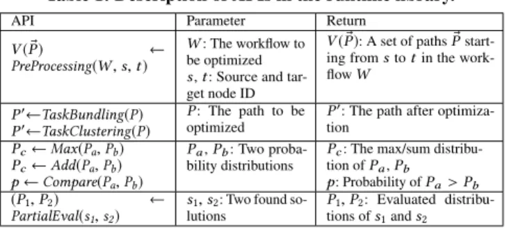
Table 1: Description of APIs in the runtime library.
API Parameter Return
V ( ®P ) ←
PreProcessing(W , s, t )
W : The workflow to be optimized s, t : Source and tar-get node ID
V ( ®P ): A set of paths ®P start-ing froms to t in the work-flowW
P′←TaskBundling(P) P′←TaskClustering(P)
P : The path to be optimized
P′: The path after optimiza-tion Pc← Max(Pa, Pb) Pc← Add(Pa, Pb) p ← Compare(Pa, Pb) Pa,Pb: Two proba-bility distributions
Pc: The max/sum distribu-tion ofPa,Pb
p: Probability of Pa> Pb (P1, P2) ←
PartialEval(s1, s2)
s1, s2: Two found so-lutions
P1, P2: Evaluated distribu-tions ofs1ands2
current window is the same as that of the previous window. We update system state calibrations at the end of every window.
To this method, one important parameter is the window size. Dif-ferent kinds of cloud dynamics may have difDif-ferent suitable window sizes. For each dynamics factor, we calculate the Bhattacharyya distance [3] between the real and predicted distributions for different window sizes using historical data. We select the window size which generates the shortest Bhattacharyya distance for the window-based distribution prediction. According to our sensitivity studies, we set this parameter to one day by default for cloud I/O and network performance distributions.
5.2
Runtime Library
We develop a runtime library to expose the pruning techniques of Prob. Table 1 summarizes the three types of APIs in the library.
Pre-processing APIs. We provide the PreProcessing() API, which implements the path enumeration, critical path pruning and path binding optimizations. It takes a workflow, a source node and a target node as input and returns a set of paths from the source node to the target node as output. The output paths are candidates of the critical path. This API can be called before the solution search.
Workflow-related APIs. We provide four APIs for the workflow-specific optimizations. The TaskBundling() and TaskClustering() APIs implement task bundling and task clustering optimizations, respectively. Each API takes a path as input, and return the optimized path with bundled/clustered nodes as output. The Max() and Add() APIs take two probability distributions as input and return their maximum and sum distributions as output, respectively. These APIs are useful for implementing the solution evaluation logic with performance objectives, e.g., calculating the workflow execution time distribution.
Distribution-related APIs. The PartialEval() API takes two found solutions as input and returns their partial evaluation results as output. The outputs can be used to compare the relative optimality of the two solutions. The comparison can be performed with the Compare()API, which takes two probability distributions as input and return their comparison result as output. Users can utilize the APIs to implement the solution searching logic, e.g., comparing the evaluations of found solutions to find a good one.
We take the budget-constrained scheduling problem as an example to show how users can modify their existing method using provided APIs. Algorithm 1 shows the modifications users need to make when incorporating probabilistic optimizations (right) into the existing search algorithm [32] introduced in Section 3.2 (left). Users mainly need to modify their state evaluation logics using our APIs (partial solution evaluation is omitted for clarity of presentation). Given a
workflowW to optimize, users first call the PreProcessing() API to get a pruned set of critical pathsP (Line 2). Given a found solution, users assign the instance configurations to each task of the workflow and call the TaskBundling() and TaskClustering() APIs to simplify the paths (Line 7). Note that, for fair comparison, we implement the pre-processing, task bundling and task clustering optimizations for both methods. The Add() and Max() APIs are used to evaluate the distributions of paths and the distribution of workflow (Line 8-15). Lines 17-19 show how to use the Compare() API to maintain the best found solution. With the APIs in the runtime library, users need little changes (highlighted with underlines) to their existing implementation in order to enable probabilistic optimizations. Algorithm 1 Static (left) and probabilistic (right) algorithms for budget-constrained scheduling on workflowW .
1:Preserve the best solutionCurBest; 2:P= PreProcessing(W , entry, exit); 3:. . . ▷State traversal 4:Given a solutions, assign instance
configura-tions insto each task inW;
5:Initialize workflow execution time astime= 0;
6:for eachpathinPdo
7: TaskBundling(TaskClustering(path)); 8: Initialize the length ofpathast = 0; 9: for each tasktkonpathdo 10: 11: 12: t = t + ttk ; 13: ift ≥ timethen 14: time=t; 15:
16:. . . ▷Evaluate the expected cost 17:ifcost ≤Bthen
18: iftime < CurBest .timethen 19:
20: CurBest= s;
21:. . . ▷Go back to state traversal
Preserve the best solutionCurBest;
P= PreProcessing(W , entry, exit); . . . ▷State traversal Given a solutions, assign instance configura-tions insto each task inW;
Define workflow execution time distribution
Time;
for eachpathinPdo
TaskBundling(TaskClustering(path)); Define the length distribution ofpathasT; for each tasktkonpathdo
iftkis the first task inpaththen
T = Ttk ; elseT= Add(T, Ttk ); ifpathis the first path inPthen
Time= T; elseTime= Max(Time,T)
. . . ▷Evaluate the expected cost ifcost ≤Bthen
if Compare(CurBest .Time, Time)> 0.5 then
CurBest= s;
. . . ▷Go back to state traversal
6
EVALUATIONS
We evaluate the effectiveness and efficiency of Prob using the budget-constraint scheduling problem as an example. Experiments on more use cases can be found in our technical report [33]. To demonstrate the effectiveness of probabilistic optimizations, we compare existing state-of-the-art workflow optimization approaches with and without Probincorporation. For efficiency, we compare the optimization overhead of Prob with the overhead of MC. We run the compared approaches on a machine with 24GB DRAM and a 6-core Intel Xeon CPU. Workflows are executed on Amazon EC2 or a cloud simulator.
6.1
Experimental Setup
Data processing workflows. We consider data processing work-flows from scientific and data analytics applications, denoted as scientific and MR workflows, respectively. They are important applications in HPC and Big Data areas.
The tested scientific workflows include the I/O-intensive Montage workflow and data-intensive CyberShake workflow. We create Montage workflows with 10,567 tasks each using Montage source code. The input data are the 2MASS J-band images covering 8-degree by 8-8-degree areas [20]. Since CyberShake is not open-sourced, we construct synthetic workflows with 1000 tasks each using the widely used workflow generator [24].
The MR workflows include two TPC-H queries, Q1 and Q9, expressed as Hive programs. Q1 is a relatively simple selection query, and Q9 involves multiple joins. Both queries have order-by
(a) Tight budget
(b) Loose budget
Figure 6: Normalized results of budget-constrained scheduling problem. Cross marks stand for budget violations.
Table 2: Hours/costs of different instance types used during one CyberShake execution under loose budget.
m1.small m1.medium m1.large m1.xlarge Average 0 0 161h/$28.4 16h/$5.7
Worst-case 507h/$22.3 0 0 0
Prob 0 0 169h/$29.6 0
and group-by operators. The input data size is around 500GB (the scale factor is 500) and is stored on the local HDFS. A Hive query is usually composed of several MR jobs. Q1 is composed of two MR jobs and Q9 is composed of seven MR jobs.
Implementation. We conduct our experiments on both real clouds and simulator to study the workflow optimization problems in a controlled and in-depth manner. On Amazon EC2, we utilize an existing workflow management system [7] to execute scientific workflows, and deploy Hadoop and Hive to run the TPC-H queries. We adopt an existing cloud simulator [32] designed based on CloudSim [4] to simulate the dynamic cloud environment. As CyberShake is not open-sourced, we use trace-driven simulations for all CyberShake evaluations.
Parameter setting. In each experiment, we submit 100 jobs for each workflow with job arrival time in a Poisson distribution (λ = 0.1 by default), which is sufficiently large for measuring the stable performance. We use four types of Amazon EC2 instances with different prices and computational capabilities, including m1.small, m1.medium, m1.large and m1.xlarge. We compare Prob with two static algorithms named Average and Worst-case, which optimize the performance of workflows using the expected and the99-th percentile of cloud dynamics distributions, respectively. The static algorithms adopt the search method [32] as shown in Algorithm 1.
We set a loose budget and a tight budget as Bmin+3B4 max and
3Bmin+Bmax
4 , respectively, whereBminandBmaxare the expected
cost of executing all tasks in the workflow on m1.small instances and on m1.xlarge instances, respectively. Given a budget, we run the compared algorithms for 100 times and compare average monetary cost and execution time results.
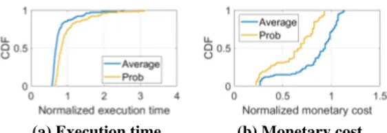
(a) Execution time (b) Monetary cost
Figure 7: Cumulative distributions of normalized execution time and monetary cost of Cybershake under loose budget.
6.2
Optimization Effectiveness
Figure 6a and 6b show the average execution time and monetary cost optimization results of the compared algorithms when the budget is set to tight and loose, respectively. The execution time results are normalized to that of Prob and the monetary cost results are normalized to the budget. In the following, the error bars show the standard deviation of the results. We have the following observations.
Compared to Worst-case, Prob obtains better performance results while satisfying the budget constraint under all settings. Prob reduces the expected execution time of Montage, CyberShake, Q1 and Q9 by 51%, N/A, 36% and N/A under the tight budget, and by 24%, 37%, 19% and 26% under the loose budget. Worst-case cannot find a feasible solution for CyberShake and Q9 under the tight budget because these two workflows are more data- and network-intensive. As Worst-case tends to over-estimate the average execution time of workflows, it always chooses cheaper instance types than Prob to guarantee the budget, as shown in Table 2. The improvement of Prob over Worst-case is larger when the budget is tight. This is because cheap instances are chosen when the budget is tight and performance variations of workflows are more severe on cheap instances.
Compared to Average, Prob is able to guarantee the budget constraint under all settings. The Average method tends to under-estimate the expected execution time of workflows. As a result, the monetary cost estimated by Average for each found solution is lower than the real cost. Differences between the cost estimated by Proband Average during solution search for Montage, CyberShake, Q1 and Q9 are up to 2%, 14%, 12% and 20%, respectively, under the tight budget. Under-estimation of the cost leads to infeasible solutions due to budget violations, as illustrated by the cross marks in Figure 6a and 6b. To further understand the impact of cloud dynamics to Average, we show the cumulative distributions of the monetary cost and execution time results of Cybershake under the loose budget. As shown in Figure 7b, among the 100 times of executions, only around 70% of results obtained by Average satisfy the budget constraint (i.e., normalized cost ≤ 1) while Prob can 100% guarantee the budget constraint.
Average performs especially poor on Q9 due to several reasons. First, due to the all-to-all structure of MR workflows, there are a large number of MAX operations when calculating the workflow execution time, which causes large errors with the static methods. Second, Q9 is composed of seven MR jobs, which is more complicated than Q1. The errors obtained on each level of Q9 accumulate and thus make Average seriously violating the budget constraint. Table 3 shows the differences between Prob and Average on the expected execution time from the entry to each level of the Q9 workflow structure.
The above observations demonstrate that, considering cloud performance dynamics gives more accurate estimations of workflow
Table 3: Differences between Prob and Average on the expected execution time from entry task to each level of Q9.
level 0 1 2 3 4 5 6 7 8-13
diff. (%) 4.8 7.4 9.4 10.5 13.7 15.9 18.3 21.5 27.6
performance in the cloud, so that budget constraints can be satisfied and better optimization results can be obtained.
6.3
Comparison with MC
We compare Prob with MC method (Section 3.3) to evaluate the effectiveness and efficiency of our pruning techniques.
Effectiveness. We calculate the average ratio of optimized results between Prob and MC. The calculated ratio is 1.05, which means that Prob achieves a close optimization result as MC and thus demonstrates the effectiveness of Prob. This is mainly due to the fact that all pruning techniques in Prob can theoretically guarantee that the input probability distributions remain the same or similar after optimizations.
Efficiency. The average optimization overhead of Prob are 2.5s, 1.7s, 6.1s and 7.0s for Montage, CyberShake, Q1 and Q9 workflows, respectively. The average speedup over MC is 450x. We take a closer look at our pruning techniques to evaluate their individual effectiveness on reducing the overhead of Prob. With the pre-processing operations, the number of paths enumerated in a workflow can be greatly reduced. For example, the pre-processing operation reduces the number of paths from219, 452 to one for the Montage workflow. The workflow-specific optimizations can reduce the path distribution evaluation overhead by 20% on average. The partial solution evaluation can reduce solution search overhead up to 78%. The above observations demonstrate that, our pruning techniques can greatly reduce the optimization overhead while maintaining the effectiveness of probabilistic optimizations.
7
RELATED WORK
Workflow optimizations in the cloud. Performance and cost opti-mizations for data-centric workflows in the cloud have been widely studied [14, 15, 18]. Mao et al. [18] proposed an auto-scaling method to maximize workflow performance in the cloud under budget constraints. Malawski et al. [15] propose to optimize for workflow ensembles under both budget and deadline constraints. Kllapi et al. [14] proposed a generic optimizer for both constrained and skyline optimization problems of dataflows in the cloud. However, none of them has considered the impact of cloud dynamics.
Dynamic cloud environment. Many existing works have studied the performance dynamics in the cloud. Previous works have demonstrated significant variances on the cloud performance [9, 27]. The distribution model (histogram) is also adopted in the previous work [27] to measure and analyze the cloud performance variances. Recently, there are some studies proposing various methods such as dynamic scheduling and stochastic modeling to address the resource provisioning problem considering cloud dynamics (or uncertainties) [29]. However, those solutions are designed for a specific goal while Prob can be adopted by different resource provisioning methods to incorporate cloud dynamics.
Efficient probabilistic methods. The probabilistic distribution model has been adopted in different research domains to improve the optimization results in dynamic environments. In database field, efficiently evaluating probabilistic queries over imprecise data is a
hot research topic. Many pruning mechanisms have been proposed to improve the efficiencies of answering probabilistic queries such as top-k [19], aggregations and nearest neighbor [21] on probabilistic databases [6]. Different from those studies, Prob is specially designed for the performance optimizations of data processing workflows. In big data processing, UP [16] is a probabilistic method which studies the uncertainty propogation in data processing systems to achieve bounded accurate data processing with uncertain data. However, this method assumes given probability distribution while Prob does not have any assumption on the distribution of cloud dynamics. 3Sigma [23] is another distribution-based method proposed for cluster scheduling considering runtime uncertainty. However, different from Prob, this work does not consider the uncertainty propagation problem in complicated job structures such as workflows, and experimented with mapper only jobs.
8
CONCLUSION
We propose a probabilistic optimization runtime named Prob for resource provisioning of workflows considering system variations. Specifically, we focus on the cloud system and model cloud dynam-icsas time-dependent random variables. Prob takes their probability distributionsas optimization input to resource provisioning problems of workflows and thus can have a better view of system performance and generate more accurate optimization results. The main challenge of Prob is the large computation overhead due to complex workflow structures and the costly distribution calculations. To address this challenge, we propose three pruning techniques to simplify workflow structure and reduce the distribution evaluation overhead. We implement our techniques in a runtime library, which allows users to incorporate efficient probabilistic optimization into their existing resource provisioning methods. Experiments on real cloud show that probabilistic solutions can improve the performance by 51% compared to state-of-the-art static solutions while guaranteeing budget constraint, and our pruning techniques can greatly reduce the overhead of probabilistic optimization. As future work, we plan to study Prob on more use cases and different systems.
ACKNOWLEDGMENT
This work is in part supported by the National Natural Science Foundation of China (No. 61802260), the Guangdong Natural Science Foundation (No. 2018A030310440), the Shenzhen Science and Technology Foundation (No. JCYJ20180305125737520) and the Natural Science Foundation of SZU (No. 000370). Bingsheng He’s research is partly supported by a MoE AcRF Tier 1 grant (T1 251RES1610) in Singapore. Reynold Cheng was supported by the Research Grants Council of HK (RGC Projects HKU 17229116, 106150091 and 17205115), the University of HK (104004572, 102009508 and 104004129) and the Innovation&Technology Com-mission of HK (ITF project MRP/029/18). Shadi Ibrahim’s work is partly supported by the ANR KerStream project (ANR-16-CE25-0014-01) and the Stack/Apollo connect talent project.
REFERENCES
[1] Bilge Acun, Phil Miller, and Laxmikant V. Kale. 2016. Variation Among Processors Under Turbo Boost in HPC Systems. In ICS ’16. 6:1–6:12. [2] Omer Adam, Young Choon Lee, and Albert Y. Zomaya. 2017. Stochastic Resource
Provisioning for Containerized Multi-Tier Web Services in Clouds. TPDS (2017). [3] A. Bhattacharyya. 1943. On a measure of divergence between two statistical populations defined by their probability distributions. Bulletin of the Calcutta Mathematical Society35 (1943), 99–109.
[4] Rodrigo N. Calheiros, Rajiv Ranjan, Anton Beloglazov, A. F. De Rose, and Rajkumar Buyya. 2011. CloudSim: A Toolkit for Modeling and Simulation of Cloud Computing Environments and Evaluation of Resource Provisioning Algorithms. Softw. Pract. Exper. 41, 1 (2011), 23–50.
[5] Reynold Cheng, Sarvjeet Singh, Sunil Prabhakar, Rahul Shah, Jeffrey Scott Vitter, and Yuni Xia. 2006. Efficient Join Processing over Uncertain Data. In CIKM ’06. [6] Nilesh Dalvi and Dan Suciu. 2007. Efficient Query Evaluation on Probabilistic
Databases. The VLDB Journal 16, 4 (2007), 523–544.
[7] Ewa Deelman, Karan Vahi, Gideon Juve, Mats Rynge, Scott Callaghan, Philip J. Maechling, Rajiv Mayani, Weiwei Chen, Rafael Ferreira da Silva, Miron Livny, and Kent Wenger. 2015. Pegasus, a workflow management system for science automation. FGCS 46 (2015), 17–35.
[8] Sheng Di, Yves Robert, Frédéric Vivien, Derrick Kondo, Cho-Li Wang, and Franck Cappello. 2013. Optimization of Cloud Task Processing with Checkpoint-restart Mechanism. In SC ’13. 64:1–64:12.
[9] Benjamin Farley, Ari Juels, Venkatanathan Varadarajan, Thomas Ristenpart, Kevin D. Bowers, and Michael M. Swift. 2012. More for Your Money: Exploiting Performance Heterogeneity in Public Clouds. In SoCC ’12.
[10] M. Reza Hoseinyfarahabady, Hamid R.D. Samani, Luke M. Leslie, Young Choon Lee, and Albert Y. Zomaya. 2013. Handling Uncertainty: Pareto-Efficient BoT Scheduling on Hybrid Clouds. In ICPP ’13. 419–428.
[11] Botong Huang and Jun Yang. 2017. Cumulon-D: data analytics in a dynamic spot market. VLDB (2017), 865–876.
[12] Qingjia Huang, Sen Su, Jian Li, Peng Xu, Kai Shuang, and Xiao Huang. 2012. Enhanced Energy-Efficient Scheduling for Parallel Applications in Cloud. In CCGRID ’12. 781–786.
[13] Iperf. 2017. https:// github.com/ esnet/ iperf . accessed on July 2017.
[14] Herald Kllapi, Eva Sitaridi, Manolis M. Tsangaris, and Yannis Ioannidis. 2011. Schedule Optimization for Data Processing Flows on the Cloud. In SIGMOD ’11. [15] Maciej Malawski, Gideon Juve, Ewa Deelman, and Jarek Nabrzyski. 2012.
Cost-and Deadline-constrained Provisioning for Scientific Workflow Ensembles in IaaS Clouds. In SC ’12. 22:1–22:11.
[16] Ioannis Manousakis, Íñigo Goiri, Ricardo Bianchini, Sandro Rigo, and Thu D. Nguyen. 2018. Uncertainty Propagation in Data Processing Systems. In SoCC. [17] Ming Mao and Marty Humphrey. 2011. Auto-scaling to Minimize Cost and Meet
Application Deadlines in Cloud Workflows. In SC ’11. Article 49, 12 pages. [18] Ming Mao and Marty Humphrey. 2013. Scaling and Scheduling to Maximize
Application Performance Within Budget Constraint in Cloud Workflows. In IPDPS’13. 67–78.
[19] Luyi Mo, Reynold Cheng, Xiang Li, David W. Cheung, and Xuan S. Yang. 2013. Cleaning uncertain data for top-k queries. In ICDE ’13. 134–145.
[20] NASA/IPAC. 2005. Montage Archive. http://hachi.ipac.caltech.edu:8080/ montage/. (2005).
[21] Johannes Niedermayer, Andreas Züfle, Tobias Emrich, Matthias Renz, Nikos Mamoulis, Lei Chen, and Hans-Peter Kriegel. 2013. Probabilistic Nearest Neighbor Queries on Uncertain Moving Object Trajectories. VLDB (2013). [22] Zhonghong Ou, Hao Zhuang, Jukka K. Nurminen, Antti Ylä-Jääski, and Pan Hui.
2012. Exploiting Hardware Heterogeneity Within the Same Instance Type of Amazon EC2. In HotCloud’12.
[23] Jun Woo Park, Alexey Tumanov, Angela Jiang, Michael A. Kozuch, and Gregory R. Ganger. 2018. 3Sigma: Distribution-based Cluster Scheduling for Runtime Uncertainty. In EuroSys ’18. 1–17.
[24] Pegasus. 2014. Workflow Generator. https://confluence.pegasus.isi.edu/display/ pegasus/WorkflowGenerator. (2014).
[25] Deepak Poola, Kotagiri Ramamohanarao, and Rajkumar Buyya. 2014. Fault-tolerant Workflow Scheduling using Spot Instances on Clouds. In ICCS ’14. [26] Martin Rinard. 2006. Probabilistic Accuracy Bounds for Fault-tolerant
Computa-tions That Discard Tasks. In ICS ’06. 324–334.
[27] Jörg Schad, Jens Dittrich, and Jorge-Arnulfo Quiané-Ruiz. 2010. Runtime Measurements in the Cloud: Observing, Analyzing, and Reducing Variance. VLDB (2010), 460–471.
[28] Gurmeet Singh, Mei-Hui Su, Karan Vahi, Ewa Deelman, Bruce Berriman, John Good, Daniel S. Katz, and Gaurang Mehta. 2008. Workflow Task Clustering for Best Effort Systems with Pegasus. In MG ’08. 9:1–9:8.
[29] Andrei Tchernykh, Uwe Schwiegelsohn, Vassil Alexandrov, and El ghazali Talbi. 2015. Towards understanding uncertainty in Cloud computing resource provisioning. In ICCS ’15. 1772–1781.
[30] Ashish Thusoo, Zheng Shao, Suresh Anthony, Dhruba Borthakur, Namit Jain, Joydeep Sen Sarma, Raghotham Murthy, and Hao Liu. 2010. Data Warehousing and Analytics Infrastructure at Facebook. In SIGMOD ’10. 1013–1020. [31] Jia Yu, Rajkumar Buyya, and Chen Khong Tham. 2005. Cost-Based Scheduling
of Scientific Workflow Applications on Utility Grids. In e-Science ’05. 140–147. [32] Amelie Chi Zhou, Bingsheng He, Xuntao Cheng, and Chiew Tong Lau. 2015.
A Declarative Optimization Engine for Resource Provisioning of Scientific Workflows in IaaS Clouds. In HPDC ’15. 223–234.
[33] Amelie Chi Zhou, Bingsheng He, Shadi Ibrahim, and Reynold Cheng. 2019. Incorporating Probabilistic Optimizations for Resource Provisioning of Cloud Workflow Processing. Technical Report 2019-TR-Prob. https://bit.ly/2ZrEGHy. 10