HAL Id: hal-01008592
https://hal.archives-ouvertes.fr/hal-01008592
Submitted on 23 Apr 2021HAL is a multi-disciplinary open access archive for the deposit and dissemination of sci-entific research documents, whether they are pub-lished or not. The documents may come from teaching and research institutions in France or abroad, or from public or private research centers.
L’archive ouverte pluridisciplinaire HAL, est destinée au dépôt et à la diffusion de documents scientifiques de niveau recherche, publiés ou non, émanant des établissements d’enseignement et de recherche français ou étrangers, des laboratoires publics ou privés.
On the Equivalent In-Plane Permeabiliy
Francisco Chinesta, Arnaud Poitou, Sylvain Chatel, Juan Antonio Garcia,
Llanos Gascón
To cite this version:
Francisco Chinesta, Arnaud Poitou, Sylvain Chatel, Juan Antonio Garcia, Llanos Gascón. On the Equivalent In-Plane Permeabiliy. 13th ESAFORM Conference on Material Forming, 2010, Brechia, Italy. pp.651-654, �10.1007/s12289-010-0854-5�. �hal-01008592�
____________________
* Francisco Chinesta: Centrale Nantes, 1 rue de la Noe, BP 92101, F-44321 Nantes cedex 3, Francisco.Chinesta@ec-nantes.fr
ON THE EQUIVALENT IN-PLANE PERMEABILITY
F. Chinesta
1*, A. Poitou
1, S. Chatel
2, J.A. Garcia
3, LL. Gascon
31
GEM, Centrale de Nantes, BP 92101, F-44321 Nantes cedex 3, France
2
EADS France Innovation Works, Allée du Chaffault, 44340 Bouguenais, France
2
Universidad Politécnica de Valencia, Camino de Vera s/n, E-46071 Valencia, Spain
ABSTRACT: Simulation of RTM processes is usually performed in 2D. Thus, only a mesh of the middle plane is
needed with the associated degrees of freedom savings with respect to fully 3D modeling. However such modeling needs the definition of an equivalent in-plane permeability representing the ignored dimension (the thickness). The definition of such permeability is not a trivial task because each ply in the thickness direction can be anisotropic, being the principal anisotropy direction different from one ply to the neighbor plies. In this work we propose a novel fully 3D modeling whose computational cost is equivalent to a 2D solution. It allows addressing properly the equivalent in-plane permeability issue.
KEYWORDS: RTM, Permeability, Separated representations, Model reduction
1 INTRODUCTION
In general the simulation of RTM processes assumes a 2D flow model. The most usual model results of combining the Darcy’s law and the flow incompressibility:
0
p
v
K
v
that results in the second order BVP:
p
0
K
The main issue in defining this model concerns the definition of the permeability tensor
K
. Different techniques exist, but in that follows we are assuming that an averaged permeability has been determined for each type of reinforcement architecture.First we are considering a laminate composed of many layers with the same principal directions, whose permeability tensor writes
0
0
0
0
K
Now, we consider the flow in a plate mould, being the permeability principal directions parallel to the mould walls. In this case the permeability tensor becomes diagonal. The simplest scenario concerns
and0
. In this case the flow is unidirectional. When the ply is placed after performing a certain in-plane rotation to the principal permeability directions, the
component of the permeability tensor is no more zero. In that case when we impose a constant injection pressure, being the pressure in the opposite mould boundary zero, the resulting pressure field is depicted in Fig. 1.
Figure 1: Pressure distribution
By computing the velocity fields associated with the pressure fields depicted in Fig. 1 we can notice significant deviation with respect to the unidirectional flow.
Now, we are analyzing another 2D situation, in which a laminate composed of different layers is considered. The principal directions of all the plies correspond to the coordinate axes, but the permeability is changing from one layer to other. Figure 2 depicts
z
, being0
,
and
constants. Figure 2 depicts theevolution of
z
.Figure 2: Evolution of the permeability in the thickness
Figure 3 depicts the pressure distribution related to the choice of the permeability. The velocity fields associated to this pressure distribution is depicted in Fig. 4
Figure 3: Pressure distribution
Figure 4: Velocity field
We can conclude that if the principal directions of the permeability of each layer are aligned along the coordinate axes, even if the permeability evolves in the thickness direction, the flow remains unidirectional. The situation is radically different if the permeability also evolves in the x-direction. When we assumes an evolution of
x z
,
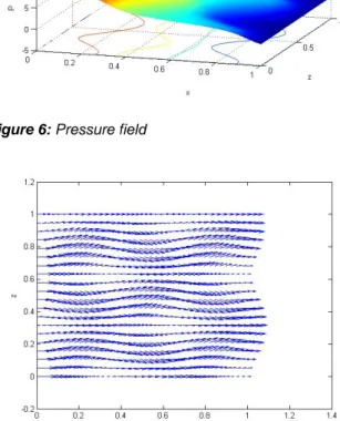
as depicted in figure 5, the pressure field that results, illustrated in figure 6, implies the velocity field depicted in figure 7, which exhibit noticeable deviations with respect to an unidirectional flow.Figure 5: Evolution of the permeability
Figure 6: Pressure field
Figure 7: Velocity field
These simple examples have proven that in general laminates, involving many layers with different reinforcement orientations the situation could be quite complex and the assumption of a simple average of the permeability of the different layers could be a crude approximation that deserves a deeper analysis. For this purpose a fully 3D simulation could be the best alternative, but an accurate representation of the thickness direction could become too expensive from the computational view point.
An appealing alternative consists in applying a separated representation of the pressure field involved in the porous media flow modelling. This kind of approximation allows computing 3D solutions with a computational cost characteristic of 2D simulations, that is, of standard RTM simulations. In the next section we
summarized the main elements of such technique, deeply described in many of our former works [1-2], and that is here particularized to the treatment of the Darcy’s model defined in plate moulds. Its extension to shell geometries is quite direct.
2 PGD IN PLATE DOMAINS
In what follows we are illustrating the construction of the Proper Generalized Decomposition of a model defined in a plate domain
I
with
2and
0,
I
H
:
p
0
K
(1)We consider that the laminate is composed of P different anisotropic plies each one characterized by a well defined permeability tensor
K
i
x y
,
-it is assumed constant in the ply thickness-. Moreover, without a loss of generality, we assume the same thickness for the different layers of the laminate, that we denotes by h. Thus, we can define a characteristic function representing the position of each layer:1
1
( )
0
i i iz
z
z
z
otherwise
,i
L
1,
,
P
(2)where
z
i
i
1
h
. Now, the laminatedpermeability can be given in the following separated form:
1, ,
i P i i ix y z
z
K
K x
(3) wherex
( , )
x y
. The weak form of Eq. (1) writes:
*0
p
p d
K
(4)with the test function
p
* in an appropriate functional space. The solutionp x y z
, ,
is searched under the separated form:
1,
i N i i ip
z
X
Z z
x
x
(5)In what follows we are illustrating the construction of one such decomposition. For this purpose we assume that at iteration
n
N
the solution is already known:
1,
i n n i i ip
z
X
Z z
x
x
(6)and that at the present iteration we look for the solution enrichment:
1,
,
( )
( )
n np
x
z
p
x
z
R
x
S z
(7)The test function involved in the weak form is searched under the form:
* * *
,
( )
( )
( )
( )
p
x
z
R
x
S z
R
x
S z
(8)By introducing Eqs. (7) and (8) into (4) it results:
°
°
°
°
°
* * * * * * * * nR S
R S
R S
d
dS
dS
dS
R
R
R
dz
dz
dz
R S
R S
d
dS
dS
R
R
dz
dz
K
Q
(9) where
°
denotes the plane component of the gradient operator
°
T
x
,
y
andQ
n denotes the flux at iteration n:°
1 i i i n n i i iX
Z z
dZ z
X
dz
x
Q
K
x
(10)Now, as the enrichment process is non-linear we propose to search the couple of functions
R x
andS z
by applying an alternating direction fixed point algorithm. Thus, assumingR x
known, we computeS z
, and then we updateR x
. The process continues until reaching convergence. The converged solutions allow defining the next term in the finite sums decomposition:
n 1
R
x
X
x
andS z
Z
n1
z
. We are illustrating each one of the just referred steps:1. Computing
R x
fromS z
:When
S z
is known the test function reduces to:
* *
,
( )
( )
p
x
z
R
x
S z
(11)and the weak form (9) reduces to:
°
°
°
* * * * nR S
R S
d
dS
dS
R
R
dz
dz
R S
d
dS
R
dz
K
Q
(12)Now, as all the functions involving the coordinate z are known, they could be integrated in
I
0,
H
. Thus, if we consider: T
k
K
k
k
(13)with xx xy yx yy
k
k
k
k
k
, xz yzk
k
k
and
k
zz, then we can define: 2 0 0 2 0 0 z H z H z z x z H z H T z zdS
S dz
Sdz
dz
dS
dS
Sdz
dz
dz
dz
k
K
k
k
(14) and °
0 0 1 0 0 z H z H i i i N z z x n i z H z H i T i i i z z dZ SZ dz S dz dz X X dZ dS dS Z dz dz dz dz dz
k x Q x k k (15) that allows writing equation (12) into the form°
°
°
* * * * x x nR
R
d
R
R
R
d
R
K
Q
(16)that defines an elliptic 2D problem defined in the middle plane of the plate.
2. Computing
S z
fromR x
:When
R x
is known the test function writes:
* *
,
( )
( )
p
x
z
R
x
S z
(17)and the weak form (9) reduces to:
°
°
°
* * * * nR S
R S
d
dS
dS
R
R
dz
dz
R S
d
dS
R
dz
K
Q
(18)Now, as all the functions involving the in-plane coordinates
x
x y
,
are known, they could be integrated in
. Thus, using the previous notation, we can define:°
°
°
°
2 zR
R
d
R
Rd
R Rd
R
d
k
K
k
k
(19) and °
°
° ° 1 i i i i N z n i i i i R X d R X d Z dZ dz R X d RX d
k Q k k (20) that allows writing equation (18) into the form* * * * z I z n I
S
S
dz
dS
dS
dz
dz
S
dz
dS
dz
K
Q
(21)that defines a one-dimensional BVP.
3 CONCLUSIONS
This paper comes back to a recurrent issue in the numerical modelling of RTM flows, the one related to the pertinence of using 2D flow models making use of an averaged permeability of the different layers involved in the laminate. In complex situations significant deviations could be found, these deviations are being studied at present, and could justify the use of a fully 3D modelling. However, 3D simulations are reputed expensive from the point of view of the computational resources required for addressing complex scenarios. The use of separated representations as the ones involved in the proper generalized decompositions –PGD- could be an appealing alternative for addressing 3D models with a cost characteristic of 2D simulations. The application of the PGD on the fully 3D simulation of flows encountered in RTM processes constitutes a work in progress.
REFERENCES
[1] A. Ammar, B. Mokdad, F. Chinesta, R. Keunings, A new family of solvers for some classes of multidimensional partial differential equations encountered in kinetic theory modeling of complex fluids, J. Non-Newtonian Fluid Mech., 139: 153-176, 2006.
[2] A. Ammar, B. Mokdad, F. Chinesta, R. Keunings, A new family of solvers for some classes of multidimensional partial differential equations encountered in kinetic theory modeling of complex fluids. Part II: transient simulation using space-time separated representations, J. Non-Newtonian Fluid