American Dairy Science Association, 2005.
Adjustment for Heterogeneous Covariance due to Herd Milk Yield
by Transformation of Test-Day Random Regressions
N. Gengler,1,2G. R. Wiggans,3and A. Gillon2
1National Fund for Scientific Research, B-1000 Brussels, Belgium
2Animal Science Unit, Gembloux Agricultural University, B-5030 Gembloux, Belgium
3Animal Improvement Programs Laboratory, Agricultural Research Service, USDA, Beltsville, MD 20705
ABSTRACT
A method of accounting for differences in covariance components of test-day milk records was developed based on transformation of regressions for random ef-fects. Preliminary analysis indicated that genetic and nongenetic covariance structures differed by herd milk yield. Differences were found for phenotypic covari-ances and also for genetic, permanent environmental, and herd-time covariances. Heritabilities for test-day milk yield tended to be lower at the end and especially at the start of lactation; they also were higher (maxi-mum of ∼25%) for high-yield herds and lower (maxi-mum of 15%) for low-yield herds. Permanent environ-mental variances were on average 10% lower in high-yield herds. Relative herd-time variances were ∼10% at start of lactation and then began to decrease regard-less of herd yield; high-yield herds increased in midlac-tation followed by another decrease, and medium-yield herds increased at the end of lactation. Regressors for random regression effects were transformed to adjust for heterogeneity of test-day yield covariances. Some animal reranking occurred because of this transforma-tion of genetic and permanent environmental effects. When genetic correlations between environments were allowed to differ from 1, some additional animal re-ranking occurred. Correlations of variances of genetic and permanent-environmental regression solutions within herd, test-day, and milking frequency class with class mean milk yields were reduced with adjustment for heterogeneous covariance. The method suggests a number of innovative solutions to issues related to het-erogeneous covariance structures, such as adjusted es-timates in multibreed evaluation.
(Key words: heterogeneous covariance, covariance structure, test-day yield, random regression)
Abbreviation key: EM = expectation maximization, HC = heterogeneous covariance, RRM = random
re-gression model.
Received December 31, 2003. Accepted May 5, 2005.
Corresponding author: N. Gengler; e-mail: gengler.n@fsagx.ac.be.
2981
INTRODUCTION
Accounting for heterogeneity of covariance among test-day observations is an important component of test-day model development. For lactation models, the issue of heterogeneous variance has been addressed by numerous studies (e.g., Dong and Mao, 1990; Short et al., 1990), and most genetic evaluation systems account for heterogeneity of variance through data adjustment prior to analysis (e.g., Wiggans and VanRaden, 1991) or direct estimation during analysis (e.g., Meuwissen et al., 1996). Only a few systems correct for heterogeneous variance components. One example is in the US, where heritability is adjusted (Wiggans and VanRaden, 1991). For test-day models, most studies have focused on heterogeneity of phenotypic (e.g., Iba´n˜ ez et al., 1996; Pool and Meuwissen, 2000) or residual (e.g., Iba´n˜ ez et al., 1999; Rekaya et al., 1999; Jaffrezic et al., 2000) variance. However, heterogeneity of covariance compo-nents, which is more difficult to estimate, has received limited attention despite its importance. The assumed covariance structures among test-day yields are used for estimation over the whole lactation or across lacta-tions, even if information is available only for a few test days (e.g., Pool and Meuwissen, 1999).
One feature of random coefficient models, also known as random regression models (RRM), is that they allow for modeling of covariances through regressions. That feature has been used in studies on heat stress (Ravag-nolo and Misztal, 2000) and on reaction norm models (Strandberg et al., 2000). With current RRM, covari-ances are modeled as functions of regression and ele-mentary covariances among regressions.
Simple, robust estimation procedures for heteroge-neous covariance (HC) matrices currently are not avail-able. The first objective of this study, therefore, was to estimate HC components according to herd milk yield. The second objective was to show that HC across herd yield levels can be modeled by adjusting a priori regres-sions for random effects. The final objective was to ex-tend the method to study and to model genetic correla-tions between herd yield levels that can be<1.
MATERIALS AND METHODS Data
Test-day milk yields (222,679) of first-parity Holstein cows in New York, Wisconsin, and California herds from 1990 through 2000 were adjusted additively to a constant age and lactation stage using the adjustment factors of Bormann et al. (2002). Those factors had been obtained from a much larger data set, of which the data for this study were a subset. The comparability of results with those from other investigations of test-day evaluation methodology with US data (Bormann et al., 2002, 2003; Gengler and Wiggans, 2002; Wiggans et al., 2002) and the availability of estimates for effect of age and lactation stage based on a large population were considered to be of sufficient benefit to offset possi-ble effects on variance reduction for random effects from data adjustment prior to analysis. Eventual shifts in the overall mean for the data were accommodated by adjusting a fixed effect so that the mean was kept in the model.
This approach also allowed the direct use of mean herd yield levels. Four data subsets of similar size (55,604 to 55,685 records) were defined by mean herd yield. Herds could change yield levels after 2 yr. Differ-ence in mean test-day milk yield of first-parity cows in the highest (37.4 kg) and lowest (23.3 kg) subsets for herd yield was 14.1 kg. The complete data set also was grouped into three randomly selected subsets, which had similar size (72,582 to 76,641 records) and mean test-day milk yield (29.0 to 30.7 kg). The three random data subsets were used to compute genetic correlations across environments, which were then averaged over the three data sets.
Covariance Structure
Consider the following RRM:
y = Xt +
∑
iQiui+ e,
where y = vector of test-day records, t = vector of fixed effects, X = incidence matrix linking y and t, Qi= matrix
of regressors, ui = vector of random effects i, and e =
vector of residuals. The test-day record is nested in a given lactation of a given animal. The covariances among observations for that lactation and animal are as follows:
Var(y) =
∑
i
QiVar(ui)Q′i+ Var(e),
which can be rewritten as
Var(y) =
∑
i
QiGiQ′i+ R,
where Gi = elementary covariance matrix for random
effects and R = Var(e); QiGiQ′icreates the covariance
components linked to random effect i in Var(y). At this stage, the matrices of regressors can be used to generate HC structures by modeling the covariances as functions of regression variables:
Var(yj) =
∑
iQijGijQ′ij+ Rj,
where Gij = covariance matrix of effect i in
environ-ment j.
At present, direct estimation of heterogeneous Gijin
an RRM is too complex for available procedures. An indirect way to estimate heterogeneous Gijis to decom-pose the matrix into orthogonal components through a transformation matrix (T), which would render Gij
independent of the heterogeneity strata (G0i = TijGijTij′) and result in
Var(yj) =
∑
iQij(Tij)−1G0i(T′ij)−1Q′ij + Rj.
Conceptually, the simple transformation of regressors
T∗ij “bends” the matrix of coefficients through Q∗ij = QijT∗ij= Qij(Tij)−1. This approach allows replacement of Gij, which differs by environment j and effect i, with a
single matrix G0ifor every random effect i. Thus, HC
structures can be modeled easily for both nongenetic and genetic random effects.
The initial underlying assumption is that genetic cor-relations between environments are unity for every transformed regression. Transformation of regressors was done independently for the different random ef-fects. Possible dependencies among the variation of some of those random effects (e.g., genetic and perma-nent environmental) were not considered.
Although several possibilities exist for T, an obvious candidate is the inverse of the lower Cholesky decompo-sition because G0ithen becomes an identity matrix. The
Cholesky matrix is also a matrix generalization of the square root of the covariances. The approach used was a simple generalization of the standardization of random effects approach used in France (Robert-Granie´ et al., 1999). The technique of rescaling random coefficients in mixed linear models so as to make them orthogonal via a Cholesky triangular transformation of the vari-ance covarivari-ance matrix has been previously reported (e.g., Groeneveld, 1994). The advantage of doing this in a random regression or random coefficient models setting is that those models allow for the direct
integra-tion of the transformaintegra-tion. The order of random sions can be chosen so that the first transformed regres-sion is defined as the standardized constant term. Rob-ert-Granie´ et al. (2002) extended this idea to heteroskedastic random regression models. For this study, heterogeneity in Gij was modeled by modeling T∗ij. However, instead of applying a generalized expecta-tion-maximization (EM) algorithm (e.g., Foulley and Quaas, 1995), T∗ijwas modeled a posteriori based on Gij
matrices obtained from the different environments, where the distinction among environments was based on a continuous variate (e.g., yield level within hetero-geneity strata). Integrated modeling similar to the methods proposed by Robert-Granie´ et al. (2002) is mathematically straightforward but was not used in the present study because of computing complexity.
Estimation of covariance components. Covari-ance components were estimated using a combination of EM and average-information REML. If positive definite values could not be obtained through average-informa-tion REML, estimates were obtained through a combi-nation of EM and average-information REML (Druet et al., 2003).
Modeling of covariance components based on herd yield. Estimated covariance components (Gij)
were transformed into lower Cholesky triangular ma-trices Lij, where i = random effect and j = herd yield
levels (environment). Every elementary element k of
Lijk (lijk) was then modeled as a constant, linear, and
quadratic function of standardized milk yield s for class mean m based on herd, test-day, and milking frequency:
lijk= α0ik+ αliksj+ α2iks2j + εijk,
where α = regression coefficient; s =−1 + 2[(m − 23.3)/ (36.8− 23.3)] = standardized milk yield when 23.3 and 36.8 kg of milk were means for lowest and highest herd-time yield classes, respectively, −1 < s < 1, and m = mean herd milk yield for a 2-yr period; and ε = residual. In matrix algebra, for every effect i, li= Sαi+ εi, or
lil ⯗ lik ⯗ link = [Ink ⊗ S] αil ⯗ αik ⯗ αink + εil ⯗ εik ⯗ εink ,
where⊗ = Kronecker product and nk= number of
non-zero elements in L.
Estimates of αik (αˆik) were obtained independently
for every effect i and every coefficient k by solving αˆik=
(S′S)−1S′lik. The solutions allowed definition of the
transformation matrix as a function of standardized yield s. Observed covariances were regressed towards expected covariances based on herd yield. This regres-sion towards expected variances is similar to the method described by Robert-Granie´ et al. (2002); how-ever, their method was integrated, and the parameters of the dispersion models were estimated using general-ized EM REML (e.g., Foulley and Quaas, 1995).
A second major difference from the method of Robert-Granie´ et al. (2002) was that the variances and covari-ances in this study were modeled with a global general-ized square-root (Cholesky triangular) transformation of the entire matrix instead of a log transformation for variances and no transformation for correlations. Modeling under the Cholesky transformation guaran-teed positive definiteness of the covariance matrices. The method of Robert-Granie´ et al. (2002) does not guar-antee correlations in the parameter space (between−1 and 1) but has the advantage of being an integrated approach. Further research should be able to merge the indirect method in this study with the direct method of Robert-Granie´ et al. (2002).
Heterogeneous error variances were modified in a similar fashion by replacing Q with an identity matrix. Mixed-model equations were then adjusted by weighting according to the assumed inverse of the resid-ual covariance of a given record.
Applied Models
Three different models were applied to the various data sets to estimate covariance components and to calculate EBV. Table 1 summarizes application of the models to the data sets.
Covariance estimation based on herd yield. The four data subsets defined by mean herd yield were used to estimate four sets of covariance components with the RRM
y = Xt + Qhh + Qaa + Qpp + e, [1]
where y = vector of test-day records for milk yield; t = vector of fixed class effects for herd, test day, and milk-ing frequency; h = vector of random effects for 2-yr time period within herd (herd-time effects); a = vector of animal effects (breeding values); p = vector of random permanent environmental effects; e = residual effect;
X = incidence matrix that links y and t; Qh, Qa, and Qp=
matrices of constant, linear, and quadratic modified Legendre polynomials (Gengler et al., 1999): r0= 1, r1=
30.5x, and r2= (5/4)0.5(3x2− 1), where x = −1 + 2[(DIM
− 1)/(365 − 1)], that link y and h, a, and p, respectively. A previous study (Gengler and Wiggans, 2001) of the same data had found that the portion of total variance
Table 1. Applied models, data sets, and analysis results.
Analysis results
Subsets based Random
Applied All on mean herd subsets
model Model description data yield (n = 4) (n = 3) 1 No heterogeneous covariance EBV Covariance —
adjustment; genetic correlation component across environments = 1 estimates
2 Heterogeneous covariance EBV — Covariance
adjustment; genetic correlation component
across environments = 1 estimates1
3 Heterogeneous covariance EBV — Covariance
adjustment; genetic correlation component
across environments≠ 1 estimates
1Computations used for likelihood ratio tests to compare Models [2] and [3].
explained by a herd-time effect was not negligible; therefore, h was included to allow herd-specific lacta-tion curves. The covariance structure for Model [1] can be summarized as Var h a p e = Ih⊗ H0 0 0 0 0 A⊗ G0 0 0 0 0 Ip⊗ P0 0 0 0 0 Inσ2e , and Var(y) = Qh(Ih⊗ H0)Qh′ + Qa(A⊗ G0)Q′a + Qp(Ip⊗ P0)Q′p+ Inσ2e,
where I = identity matrix; H0, G0, and P0= elementary
covariance matrices among the three random regres-sions for herd-time, genetic, and permanent environ-mental effects, respectively; A = additive relationship matrix, h = number of herd-time effects, p = number of animals with records, and n = number of test-day records.
Second-order polynomials were used as a compromise between model complexity and desire to achieve a rea-sonably good fit. Preliminary research had shown that the constant, linear, and quadratic polynomials were highly related to the first, second, and third eigenvec-tors, which explained a large part of the variances for all three random effects.
Computation of EBV with and without HC ad-justment. The complete data set was analyzed with and without HC adjustment. To provide EBV without HC adjustment, the regular mixed-model equations from Model [1] were solved using mean coefficients (lijk=
α0ik). To provide EBV with HC adjustment, mixed-model equations with transformed regressors based on standardized milk yield s were solved:
y = Xt + Q∗h(s)h∗+ Q∗a(s)a∗+ Q∗p(s)p∗+ w(s)e∗, [2]
where Q∗h(s), Q∗a(s), and Q∗p(s)= matrices of transformed
regressors dependent on standardized herd yields s and linking y with h∗, a∗, and p∗and w(s) = square root of
the inverse of the weight dependent on s. The associated covariance structure was
Var h∗ a∗ p∗ e∗ = Ih⊗ I3 0 0 0 0 A⊗ I3 0 0 0 0 Ip⊗ I3 0 0 0 0 W ,
where W = Inw2(s), a diagonal matrix with diagonal
ele-ments equal to the inverse of the weight associated with the record. Covariance of the observations based on s was
Var(y(s)) = Q∗h(s)(Ih⊗ I3)Q∗′h(s)+ Q∗a(s)(A⊗ I3)Q∗′a(s)
+ Q∗p(s)(Ip⊗ I3)Q∗′p(s)+ Inw(s)2.
Genetic correlation across environments≠ 1. Al-though Model [2] allows for differences in genetic covar-iance across herd yield levels, it does not allow genetic correlation across environments to differ from 1. Re-cently, several studies (e.g., Castillo-Juarez et al., 2002) used RRM as an approach to address this issue.
Model [2] could be generalized by including separate genetic effects for high and low yield. Every observation then potentially would be influenced by two sets of ge-netic effects. Gege-netic effects for every animal then could be defined continuously from high to low yield as a∗(s)=
φ1(s)a∗1+ φ2(s)a∗2, where φ1and φ2are coefficients for
envi-ronments defined as a function of s with φ1(s)= (1 + s)/
2 and φ2(s) = 1 − φ1(s) = (1 − s)/2. The coefficients φ1(s)
obser-vation was at the maximal herd yield level (s = 1), then
φ1(1) = 1 and φ2(1) = 0; if an observation was at the
minimal low herd yield level (s = −1), then φ1(−1)= 0
and φ2(−1)= 1.
Given those conventions, Model [2] easily was rewrit-ten to allow differences in covariances across environ-ments and also genetic correlations that differed from 1:
y(s)= Xt + Q∗h(s)h + φ1(s)Q∗a(s)a∗1 [3]
+ φ2(s)Q∗a(s)a∗2+ Q∗p(s)p + w(s)e∗.
Covariance matrices for Model [3] were as follows:
Var h∗ a∗1 a∗2 p∗ e∗ = Ih⊗ I3 0 0 0 0 A ⊗ I3 D D I3 0 0 0 0 Ip⊗ I3 0 0 0 0 In , and Var(y(s)) = Q∗h(s)(Ih⊗ I3)Q∗′h(s) + φ1(s)Q ∗ a(s) φ2(s)Q∗a(s) A ⊗ I3 D D I3 φ1(s)Q∗′a(s) φ2(s)Q∗′a(s) + Q∗p(s)(Ip⊗ I3)Q∗′p(s)+ Inw2(s),
where D = diag[φk] is a diagonal matrix of dimension 3 with the correlation between transformed regressors in the two environments. In Model [3], differences in covariances across environments were accounted for by the Cholesky transformation as in Model [2]; however, correlations across environments that differed from 1 were modeled based on separation into environmentally dependent genetic effects. Covariance of the total ge-netic effects could be written as
Var(a∗p(s)) = [φ1(s) φ2(s)] A⊗ I3 D D I3 φ1(s) φ2(s) = φ21(s)(A⊗ I3) + (φ2(s)2 )(A⊗ I3) + 2φ1(s)φ2(s)(A⊗ D).
When the correlation between transformed regressors in the two environments tended to 1, covariance of the total genetic effects simplified to
Var(a∗(s)) = (φ21(s)+ φ2(s)2 + 2φ1(s)φ2(s))(A⊗ I3)
= (φ1(s)+ φ2(s))2(A⊗ I3) = A⊗ I3
as in Model [2].
To determine if the introduction of a genetic correla-tion across environments that differed from 1 improved model fit, likelihood ratio tests were conducted with covariance components estimated from each of the three random data subsets using Models [2] and [3].
The estimated covariance components from Model [3] were applied to calculate EBV for the complete data set.
Comparison of EBV
To demonstrate applicability of the methods and models, EBV were computed and expressed on a 305-d lactation basis; EBV from Mo305-dels [2] an305-d [3], which included transformation, were back-transformed to a mean scale. For cows, the same reverse transformation was done for the sum of EBV and permanent environ-mental effects. For genetic correlation ≠ 1, EBV for every animal were defined continuously from high to low yield as a∗(s) = φ1(s)a∗1+ φ2(s)a∗2, where φ1(s) + φ2(s) =
1, and reported for three environments: high herd yield (φ1(1)= 1; φ2(1)= 0), medium herd yield (φ1(0)= 0.5; φ2(0)=
0.5), and low herd yield (φ1(−1)= 0; φ2(−1)= 1). Rankings were created for cows and for sires with≥10 daughters based on unadjusted EBV, HC-adjusted EBV with netic correlation = 1, and HC-adjusted EBV with ge-netic correlation≠ 1.
One consequence of not applying adjustments for het-erogeneity of covariance is that solutions in high-vari-ance environments are more variable than in low-vari-ance environments. To test if the proposed HC adjust-ment method corrects this problem, variances of regression solutions for genetic and permanent environ-mental effects were computed in every herd, test-day, and milking-frequency class and compared with mean milk yield for that class. If the HC adjustment was successful, correlation between those variances and class mean yield should be reduced.
RESULTS AND DISCUSSION Covariance Components Based on Herd Yield
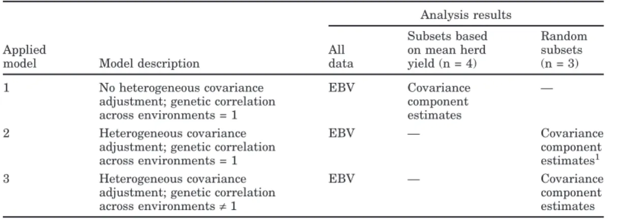
Covariance components were estimated with Model [1] and then modeled and expressed as functions of s. For simplicity, only mean variances with s = 0 (without HC adjustment) and extreme variances with s =−1 or s = 1 (with HC adjustment) are reported. Heritabilities for test-day milk yields (Figure 1) were substantially higher for high-yield than for low-yield herds and reached∼25% compared with ∼15%, respectively. Me-dium-yield herds had intermediate heritability. How-ever, the heritability trends were only somewhat simi-lar to trends for permanent-environmental variance (Figure 2) as only high-yield herds differed
substan-Figure 1. Heritability of test-day milk yield by DIM for herds
with low (×), medium (䊏), or high (䊉) yield.
tially with lower relative permanent-environmental variance compared with herds with other yield levels. Combined variance for genetic and permanent environ-mental effects may be similar across herd yields, but a larger portion of that combined variance may be genetic for high-yield herds.
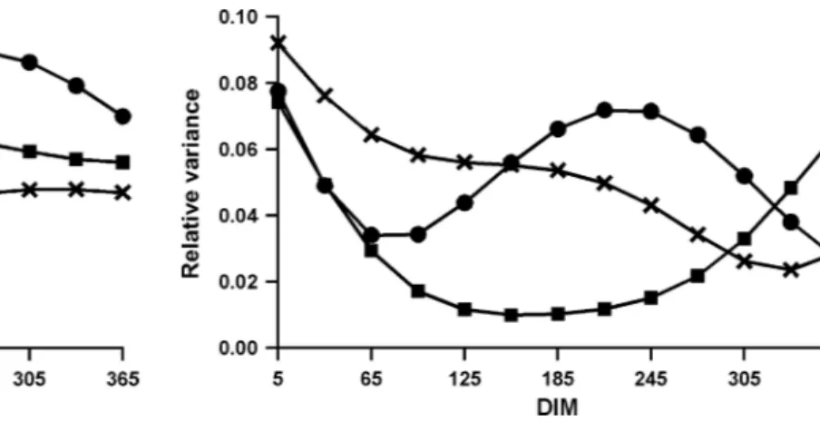
Relative herd-time variances (Figure 3) did not show similar patterns. Low-yield herds had higher herd-time variance at start of lactation, whereas variance for me-dium-yield herds was higher at start and end of lacta-tion. For high-yield herds, variance was high at the start of lactation, decreased until about 65 DIM, and then increased until around 220 DIM to the same vari-ance level as at the start of lactation, and again de-creased through the end of lactation. No explanation was apparent for the differing relative variance pat-terns, and additional research is required to investigate possible negative effects.
Figure 2. Relative variance of permanent environmental effect
on test-day milk yield by DIM for herds with low (×), medium (䊏), or high (䊉) yield.
Figure 3. Relative variance of herd-time effect on test-day milk
yield by DIM for herds with low (×), medium (䊏), or high (䊉) yield.
Relative variance patterns should be considered to-gether with the pattern for phenotypic variance (Figure 4) over lactation. Plots for phenotypic variance were similar in shape but clearly not identical across herd yield levels. For low-yield herds, variances were nearly constant with rather limited increases at start and end of lactation. Compared with low-yield herds, phenotypic variances for medium-yield herds tended to be higher and increase more at the end of lactation. For high-yield herds, overall phenotypic variance and rate of increase in variance with DIM was substantially greater than for the other yield levels. The variance increase with herd yield level could result primarily from better management in high-yield herds, which al-lowed cows to express differences. The large heritability difference seems to confirm that animals in high-yield herds express relatively more genetic variance than do those in low-yield herds. The results of this study support that lactation stage and herd yield level should
Figure 4. Phenotypic variance of test-day milk yield by DIM for
Figure 5. Phenotypic correlation of test-day milk yield at 5 DIM
with test-day yield at other DIM for herds with low (×), medium (䊏), or high (䊉) yield.
be considered when developing adjustments for hetero-geneity of phenotypic covariance.
Test-day milk yield at 5 DIM was compared with test-day yield at other DIM. Although phenotypic correla-tions (Figure 5) were remarkably stable, genetic corre-lations (Figure 6) decreased with herd yield level, espe-cially for low-yield herds. Using inflated correlations could impact animal rankings, especially for dairy bulls with early evaluations based primarily on daughter re-cords from early lactation in low-yield herds.
Estimation of Genetic Correlations Across Environments
Likelihood ratio tests for the three random data sub-sets used to compare Models [2] and [3] showed that in all cases the introduction of additional parameters in
Figure 6. Genetic correlation of test-day milk yield at 5 DIM with
test-day yield at other DIM for herds with low (×), medium (䊏), or high (䊉) yield.
the models significantly (P < 0.001) improved the fit; likelihood ratios were 75.93, 84.24, and 65.15.
Means of estimated REML genetic correlations across environments from the three random data subsets were 0.972, 0.799, and 0.968 for the three Legendre coeffi-cients. Standard deviations were 0.025, 0.211, and 0.041, respectively, which indicated a rather large de-gree of uncertainty in the estimation of the correlation for the second regression. Because of the variation in subset genetic correlations, no definitive conclusions can be made about genetic × environmental interac-tions. Genetic differences across environments were re-ported by Veerkamp and Goddard (1998). In this study, the definition of environments and data sampling based solely on mean herd yield did not allow identification of the primary reason for genetic correlations of<1. A recent study by Raffrenato et al. (2003) suggests that regional differences can be a factor, and data for this study were pooled from three states with quite different environmental conditions.
Comparison of Rankings With and Without HC Adjustment
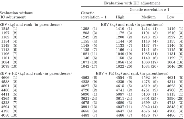
Rank correlations of cow evaluations with and with-out HC adjustment were >0.99 for EBV and >0.98 for permanent environmental effect. However, some re-ranking did occur for the top 10 cows (Table 2) and for the top 10 bulls with≥10 daughters with records (Table 3). The most reranking occurred for EBV plus perma-nent environmental effects (Table 2). Although EBV were quite stable (probably because families of animals seldom were concentrated in one environment and ties existed through the relationship matrix), HC adjust-ment resulted in some reranking of the top bulls based on evaluations without adjustment. Four (genetic corre-lation = 1) and 5 (genetic correcorre-lation≠ 1) bulls of the original top 10 were eliminated.
For genetic correlation≠ 1, all animals had breeding values across all environments because of the continu-ous description of genetic effects as a function of stan-dardized milk yield. As shown in Tables 2 and 3, animal rankings differed by mean herd yield. Evaluations of some of the top 10 bulls based on evaluations without HC adjustment were greatly affected by HC adjust-ment, with changes up to 121 kg between low- and high-yield environments. With additional research to verify the level of correlation across environments, this ob-served difference could lead to the use of the proposed HC adjustment method to create a ranking of bulls specific to a herd based on the yield level of that herd (Castillo-Juarez et al., 2002).
Table 2. Comparison of EBV, EBV plus permanent environmental (PE) effects, and rankings for evaluations
with and without heterogeneous covariance (HC) adjustment and considering genetic correlation across environments and mean herd yield (low, medium, or high) for top 10 cows.
Evaluation with HC adjustment Genetic correlation≠ 1 Evaluation without Genetic
HC adjustment correlation = 1 High Medium Low EBV (kg) and rank (in parentheses) EBV (kg) and rank (in parentheses)
1245 (1) 1398 (1) 1410 (1) 1414 (1) 1419 (1) 1197 (2) 1203 (3) 1172 (3) 1191 (3) 1210 (3) 1182 (3) 1242 (2) 1200 (2) 1213 (2) 1227 (2) 1154 (4) 1155 (4) 1144 (6) 1148 (4) 1153 (4) 1149 (5) 1148 (5) 1133 (7) 1137 (7) 1140 (5) 1143 (6) 1135 (7) 1166 (4) 1141 (5) 1115 (9) 1106 (7) 1081 (11) 1040 (19) 1085 (11) 1131 (6) 1101 (8) 1146 (6) 1150 (5) 1140 (6) 1129 (7) 1084 (9) 1071 (13) 1056 (15) 1060 (17) 1064 (16) 1079 (10) 1042 (17) 1022 (20) 1034 (20) 1046 (20) EBV + PE (kg) and rank (in parentheses) EBV + PE (kg) and rank (in parentheses)
4606 (1) 4563 (6) 4554 (6) 4592 (6) 4631 (5) 4538 (2) 4238 (9) 4239 (9) 4276 (9) 4314 (8) 4501 (3) 4627 (5) 4615 (5) 4619 (5) 4623 (6) 4480 (4) 4720 (2) 4741 (2) 4751 (2) 4760 (2) 4411 (5) 5090 (1) 5087 (1) 5100 (1) 5113 (1) 4365 (6) 3621 (24) 3611 (24) 3601 (25) 3590 (28) 4328 (7) 4675 (3) 4680 (3) 4699 (3) 4718 (3) 4204 (8) 3991 (13) 4037 (11) 3942 (14) 3848 (18) 4195 (9) 4655 (4) 4647 (4) 4676 (4) 4706 (4) 4050 (10) 4483 (7) 4466 (7) 4476 (7) 4486 (7)
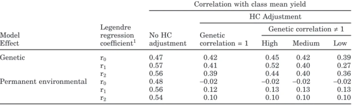
Comparison of Class Variances With and Without HC Adjustment
Correlations of variances of random regression solu-tions for genetic and permanent environmental effects within herd, test-day, and milking-frequency class with class mean yields (Table 4) were smaller with HC ad-justment than without it. The reduction in correlation was much smaller for genetic than for permanent envi-ronmental solutions (for which correlations became nearly 0). The anticipated reason for the difference in
Table 3. Comparison of EBV and rankings for evaluations with and without heterogeneous covariance (HC)
adjustment and considering genetic correlation across environments and mean herd yield (low, medium, or high) of daughter for top 10 bulls with≥10 daughters with records.
EBV (kg) and rank (in parentheses) based on evaluation with EBV (kg) and rank
HC adjustment (in parentheses)
based on evaluation Genetic correlation≠ 1 without HC Daughters Genetic
adjustment (no.) correlation = 1 High Medium Low 1099 (1) 54 1111 (1) 1168 (1) 1132 (1) 1097 (1) 984 (2) 67 921 (2) 961 (2) 929 (2) 896 (3) 926 (3) 159 900 (3) 920 (3) 907 (3) 893 (5) 898 (4) 10 851 (7) 832 (7) 844 (8) 855 (9) 869 (5) 21 776 (18) 769 (17) 783 (16) 796 (16) 867 (6) 141 869 (5) 862 (4) 857 (5) 851 (10) 861 (7) 10 842 (9) 839 (6) 838 (9) 836 (12) 856 (8) 222 803 (11) 750 (20) 790 (15) 829 (13) 829 (9) 12 825 (10) 773 (15) 832 (10) 892 (6) 823 (10) 16 756 (21) 771 (16) 776 (19) 782 (21)
the effect of HC adjustment for genetic and permanent environmental effects was the assumption of a perfect genetic correlation across environments. However, even with genetic correlation≠ 1 (Table 4), a similar pattern was observed. If the effect of HC adjustment was small, only a few animal rankings would change as was ob-served in the example data sets (Tables 2 and 3). Corre-lations for genetic solution variances with class mean yield were reduced somewhat with HC adjustment and were smallest for low-yield herds.
Table 4. Correlations of variances of random regression solutions for genetic and permanent environmental
effects within herd, test-day, and milking-frequency class with class mean yields with and without heteroge-neous covariance (HC) adjustment and considering genetic correlation across environments and mean herd yield (low, medium, or high).
Correlation with class mean yield HC Adjustment
Legendre Genetic correlation≠ 1
Model regression No HC Genetic
Effect coefficient1 adjustment correlation = 1 High Medium Low
Genetic r0 0.47 0.42 0.45 0.42 0.39 r1 0.57 0.41 0.52 0.40 0.27 r2 0.56 0.39 0.44 0.40 0.36 Permanent environmental r0 0.48 −0.02 −0.02 −0.02 −0.02 r1 0.56 0.12 0.13 0.13 0.13 r2 0.54 0.10 0.10 0.10 0.10 1r
0= 1, r1= 30.5x, and r2= (5/4)0.5(3x2− 1), where x = −1 + 2[(DIM − 1)/(365 − 1)].
CONCLUSIONS
Currently, the methods used for HC adjustment in genetic evaluations with test-day models are often pre-adjustments (International Bull Evaluation Service, 2004). Some evaluation centers are testing or consider-ing methods (e.g., Lidauer and Ma¨ntysaari, 2001) based on the approach of Meuwissen et al. (1996), but no country is yet adjusting regressions. Although this study was not directly related to current HC adjustment methods, some of its results could influence the choice of future methods. Genetic and nongenetic covariance structures were found to be different according to herd milk yield. Differences were found not only for pheno-typic covariances but also for heritability, permanent environmental, and herd-time variances. Current ad-justment methods used by all major dairy countries except the US and The Netherlands (International Bull Evaluation Service, 2004) consider the variance ratios to be constant. High-yield herds had higher heritabilit-ies for test-day milk yields and lower relative perma-nent environmental variances.
All currently used adjustment methods either correct data prior to analysis or have been integrated into the evaluation system and affect variances. This study showed that a method based on transformed regressors for random regression effects can be used to address the issue of heterogeneity of test-day yield covariances. As shown in the example data sets, some animal re-ranking occurred because of the effect of this transfor-mation on both genetic and permanent environmen-tal effects.
A challenge in the developed HC adjustment method is that nongenetic and genetic covariance matrices have to be estimated for different environments prior to cal-culation of genetic evaluations. Those additional calcu-lations could require substantial computing resources and time, and the estimates could have large sampling
errors. However, as shown with Model [3], the method can be adapted to allow genetic correlations between environments to differ from 1, which produced animal reranking in the example data sets. Correlations of re-gression coefficient variances for genetic and perma-nent environmental effects within herd, test-day, and milking frequency class with class mean milk yield were reduced with HC adjustment.
The HC adjustment method that was developed sug-gests innovative solutions for a number of issues related to heterogeneity of covariances and their impact on genetic evaluation systems. First, the general concept can be used for data adjustment both prior to analysis (single transformation of regressors) and during analy-sis (transformation and update of transformation ma-trices). Because every regression of each test-day yield of a given cow can be adjusted, extreme flexibility can be achieved within the modeling process. For example, differences in covariance structures among breeds can be accommodated for multibreed evaluation. Crossbred animals can then be included by interpolation based on the proportion of genes from each breed of ancestors. This particular benefit could be especially important if breeds are to be evaluated together because of their simultaneous presence in contemporary groups or the presence of crossbreds in contemporary groups (e.g., Jerseys and Holsteins in the US and dual-purpose Bel-gian Blues and Holsteins in Belgium). The method de-veloped also allows genetic correlations between envi-ronments to differ from 1 and has potential use if differ-ent bull rankings are needed according to source of covariance differences.
ACKNOWLEDGMENTS
Nicolas Gengler, who is a research associate of the National Fund for Scientific Research (Brussels, Bel-gium), acknowledges the Fund’s financial support and
the facilitation of computations through Grant 2.4507.02 F (2). Partial financial support for A. Gillon was provided by the Luxembourgian Herdbook Federa-tion, a breeders’ cooperative. The authors gratefully acknowledge computer programs provided by I. Misztal (University of Georgia, Athens) and T. Druet (Institut National de la Recherche Agronomique, Jouy-en-Josas, France) and manuscript review by L. L. M. Thornton and S. M. Hubbard (Animal Improvement Programs Laboratory, ARS, USDA, Beltsville, MD).
REFERENCES
Bormann, J., G. R. Wiggans, T. Druet, and N. Gengler. 2002. Estimat-ing effects of permanent environment, lactation stage, age, and pregnancy on test-day yield. J. Dairy Sci. 85(Jan.). Online. Avail-able: http://jds.fass.org/.
Bormann, J., G. R. Wiggans, T. Druet, and N. Gengler. 2003. Within-herd effects of age at test day and lactation stage on test-day yields. J. Dairy Sci. 86:3765–3774.
Castillo-Juarez, H., P. A. Oltenacu, and E. G. Cienfuegos-Rivas. 2002. Genetic and phenotypic relationships among milk production and composition traits in primiparous Holstein cows in two different herd environments. Livest. Prod. Sci. 78:223–231.
Dong, M. C., and I. L. Mao. 1990. Heterogeneity of (co)variance and heritability in different levels of intraherd milk production vari-ance and of herd average. J. Dairy Sci. 73:843–851.
Druet, T., F. Jaffre´zic, D. Boichard, and V. Ducrocq. 2003. Modeling lactation curves and estimation of genetic parameters for first lactation test-day records of French Holstein cows. J. Dairy Sci. 86:2480–2490.
Foulley, J. L., and R. L. Quaas. 1995. Heterogeneous variances in Gaussian linear mixed models. Genet. Sel. Evol. 27:211–228. Gengler, N., A. Tijani, G. R. Wiggans, and I. Misztal. 1999. Estimation
of (co)variance function coefficients for test day yield with expecta-tion-maximization restricted maximum likelihood algorithm. J. Dairy Sci. 82(June). Online. Available: http://jds.fass.org/. Gengler, N., and G. R. Wiggans. 2001. Variance of effects of lactation
stage within herd by herd yield. J. Dairy Sci. 84(Suppl. 1):216. (Abstr.)
Gengler, N., and G. R. Wiggans. 2002. Adjustment for heterogeneous genetic and non-genetic (co)variance structures in test-day mod-els using a transformation on random regression effect regressors. Interbull Bull. 29:79–83.
Groeneveld, E. 1994. A reparameterization to improve numerical optimization in multivariate REML (co)variance component esti-mation. Genet. Sel. Evol. 26:537–545.
Iba´n˜ ez, M. A., M. J. Caraban˜ o, and R. Alenda. 1999. Identification of sources of heterogeneous residual and genetic variances in milk yield data from the Spanish Holstein-Friesian population and impact on genetic evaluation. Livest. Prod. Sci. 59:33–49.
Iba´n˜ ez, M. A., M. J. Caraban˜ o, J. L. Foulley, and R. Alenda. 1996. Heterogeneity of herd-period phenotypic variances in the Spanish Holstein-Friesian cattle: Sources of heterogeneity and genetic evaluation. Livest. Prod. Sci. 45:137–147.
International Bull Evaluation Service. 2004. Description of National Genetic Evaluation systems for dairy cattle traits as applied in different Interbull member countries. Available: http://www-interbull.slu.se/national_ges_info2/framesida-ges.htm. Accessed June 20, 2004.
Jaffrezic, F., I. M. S. White, R. Thompson, and W. G. Hill. 2000. A link function approach to model heterogeneity of residual vari-ances over time in lactation curve analyses. J. Dairy Sci. 83:1089–1093.
Lidauer, M., and E. A. Ma¨ntysaari. 2001. A multiplicative random regression model for test-day data with heterogeneous variances. Interbull Bull. 27:167–171.
Meuwissen, T. H. E., G. de Jong, and B. Engel. 1996. Joint estimation of breeding values and heterogeneous variances of large data files. J. Dairy Sci. 79:310–316.
Pool, M. H., and T. H. E. Meuwissen. 1999. Prediction of daily milk yields from a limited number of test days using test day models. J. Dairy Sci. 82:1555–1564.
Pool, M. H., and T. H. E. Meuwissen. 2000. Reduction of the number of parameters needed for a polynomial random regression test-day model. Livest. Prod. Sci. 64:133–145.
Raffrenato, E., R. W. Blake, P. A. Oltenacu, J. Carvalheira, and G. Licitra. 2003. Genotype by environment interaction for yield and somatic cell score with alternative environmental definitions. J. Dairy Sci. 86:2470–2479.
Ravagnolo, O., and I. Misztal. 2000. Genetic component of heat stress in dairy cattle, parameter estimation. J. Dairy Sci. 83:2126–2130. Rekaya, R., M. J. Caraban˜ o, and M. A. Toro. 1999. Use of test day yields for the genetic evaluation of production traits in Holstein-Friesian cattle. Livest. Prod. Sci. 57:203–217.
Robert-Granie´, C., B. Bonaı¨ti, D. Boichard, and A. Barbat. 1999. Accounting for variance heterogeneity in French dairy cattle ge-netic evaluation. Livest. Prod. Sci. 60:343–357.
Robert-Granie´, C., B. Heude, and J. L. Foulley. 2002. Modelling the growth curve of Maine-Anjou beef cattle using heteroskedastic random coefficients models. Genet. Sel. Evol. 34:423–445. Short, T. H., R. W. Blake, R. L. Quaas, and L. D. Van Vleck. 1990.
Heterogeneous within-herd variance. 1. Genetic parameters for first and second lactation milk yields of grade Holstein cows. J. Dairy Sci. 73:3312–3320.
Strandberg, E., R. Kolmodin, P. Madsen, J. Jensen, and H. Jorjani. 2000. Genotype by environment interaction in Nordic dairy cattle studied by use of reaction norms. Interbull Bull. 25:41–45. Veerkamp, R. F., and M. E. Goddard. 1998. Covariance functions
across herd production levels for test day records on milk, fat, and protein yields. J. Dairy Sci. 81:1690–1701.
Wiggans, G. R., and P. M. VanRaden. 1991. Method and effect of adjustments for heterogeneous variance. J. Dairy Sci. 74:4350– 4357.
Wiggans, G. R., P. M. VanRaden, J. Bormann, J. C. Philpot, T. Druet, and N. Gengler. 2002. Deriving lactation yields from test-day yields adjusted for lactation stage, age, pregnancy, and herd test date. J. Dairy Sci. 85(Jan.). Online. Available: http://jds.fass.org/.